How opening a hole affects the sound of a flute
A one-dimensional mathematical model for a tube with a small hole pierced on its side

Abstract

In this paper, we consider an open tube of diameter $\varepsilon>0$, on the side of which a small hole of size $\varepsilon^{2}$ is pierced. The resonances of this tube correspond to the eigenvalues of the Laplacian operator with homogeneous Neumann condition on the inner surface of the tube and Dirichlet one the open parts of the tube. We show that this spectrum converges when $\varepsilon$ goes to $0$ to the spectrum of an explicit one-dimensional operator. At a first order of approximation, the limit spectrum describes the note produced by a flute, for which one of its holes is open.
Key words: thin domains, convergence of operators, resonance, mathematics for music and acoustic.
AMS subject classification: 35P15, 35Q99.

1 Introduction and main result

In this paper, we obtain a one-dimensional model for the resonances of a tube with a small hole pierced on its side. Our arguments are based on recent thin domain techniques of [18]. We show that this kind of techniques applies to the mathematical modelling of music instruments.

Basic facts on wind instruments.
The acoustic of flutes is a large subject of research for acousticians. Basically, a flute is the combination of an exciter which creates a periodic motion (a fipple, a reed etc.) and a tube, whose first mode of resonance selects the note produced. Studying the acoustic of a flute combines a lot of problems as the influence of the shape of the tube, the study of the creation of oscillations by blowing in the fipple…see [22], [11], [9], [25] and [5] for nice introductions. In this paper, we will not consider the creation of the periodic excitation, we rather want to study mathematically the resonances of the tube of the flute and how an open hole affects it. Therefore, we simplify the problem by making the following usual assumptions:
- the pressure of the air in the tube follows the wave equation and therefore the resonances of the tube are the squareroots of the eigenvalues of the corresponding Laplacian operator.
- on the inner surface of the tube, the pressure satisfies homogeneous Neumann boundary condition.
- where the tube is open to the exterior, we assume that the pressure is equal to the exterior pressure which may be assumed to be zero without loss of generality.

We can roughly classify the tube of the wind instruments in three different categories, depending on which end of the tube is open. See Figure 1.

	Sketch of the tube (the open parts are in grey)	main resonance mode	frequencies
flute, recorder, open organ pipe…			$\pi/L$, $2\pi/L$, $3\pi/L$ …
closed organ pipe, panpipes…			$\pi/2L$, $3\pi/2L$, $5\pi/2L$ …
reed instruments (clarinet, oboe…)			$\pi/2L$, $3\pi/2L$, $5\pi/2L$ …

Figure 1: Three different kind of tubes without holes and their resonances.

It is known since a long time that the resonances of the tubes of Figure 1 can be approximated by the spectrum of the one-dimensional Laplacian operator on $(0,L)$ with either Dirichlet or Neumann boundary conditions, depending on whether the corresponding end is open or not (see for example [8]). Notice that this rough approximation can explain simple facts: a tube with a closed end sounds an octave lower than an open tube of the same length (enabling for example to make shorter organ pipes for low notes) and moreover it produces only the odd harmonics (explaining the particular sounds of reed instruments).

In this article, we study how the one-dimensional limit is affected by opening one of the holes of the flute, say a hole at position $a\in(0,L)$. At first sight, one may think that it is equivalent to cutting the tube at the place of the open hole. In other words, the note is the same as the one produced by a tube of length $a$. This is roughly true for flutes with large holes as the modern transverse flute, except that one must add a small correction and the length $\tilde{a}$ of the equivalent tube is slightly larger than $a$. This length $\tilde{a}$ is called the effective length. This kind of approximation seems to be the most used one by acousticians. It states that the resonances of the tube with an open hole are: a fundamental frequency $\pi/\tilde{a}$ and harmonics $k\pi/\tilde{a}$, $k\geq 2$. However, the approximation of the resonances by the ones of a tube of length $\tilde{a}$ is too rough for flutes with small holes as the baroque flute or the recorder. In particular, the approximation by effective length fails to explain the following observations, for which we refer e.g. to [4] and [26]:
- the effective length depends on the frequency of the waves in the tube. In other words, the harmonics are not exact multiples of the fundamental frequency.
- closing or opening one of the holes placed after the first open hole of the tube changes the note of the flute. This enables to obtain some notes by fork fingering, as it is common in baroque flute or recorder. We also enhance that some effects of the baroque flute or of the recorder are produced by half-holing, that is that by half opening a hole (some flutes have even holes consisting in two small close holes to make half-holing easier). In these cases, the effective length $\tilde{a}$ is not only related to the position $a$ of the first open hole, which makes the method of approximation by effective length less relevant.

The purpose of this article is to obtain an explicit one-dimensional mathematical model for the flute with a open hole, which could be more relevant in the case of small holes than the approximation by effective length. The models used by the acousticians are based on the notion of impedance. The model introduced here rather uses the framework of differential operators.

The thin domains techniques.
The fact that the behaviour of thin three dimensional objects as a rope or a plate can be approximated by one- or two-dimensional equations has been known since a long time, see [12] and [8] for example. In general, a thin domain problem consists in a partial differential equation $(E_{\varepsilon})$ defined in a domain $\Omega_{\varepsilon}$ of dimension $n$, which has $k$ dimensions of negligible size with respect to the other $n-k$ dimensions. The aim is then to obtain an approximation of the problem by an equation $(E)$ defined in a domain $\Omega$ of dimension $n-k$. It seems that the first modern rigorous studies of such approximations mostly date back to the late 80’s: [15], [1], [2], [13], [23]… There exists an enormous quantity of papers dealing with thin domain problems of many different types. We refer to [20] for a presentation of the subject and some references.

In this paper, the domain $\Omega_{\varepsilon}$ is the thin tube of the flute and we hope to model the behaviour of the internal air pressure by a one-dimensional equation. It is well known that the wave equation in a simple tube can be approximated by the one-dimensional wave equation. Even the case of a far more complicated domain squeezed along some dimension is well understood, see [19] and the references therein. We will assume in this paper that the open parts of the tube yield a Dirichlet boundary condition for the pressure in the tube. In fact, we could study the whole system of a thin tube connected to a large room and show that, at a first order of approximation, the effect of the connection with a large domain is the same as a the one of a Dirichlet boundary condition, see [3], [2], [14] and the other works related to the “dumbbell shape” model. The main difficulty of our problem comes from the different scales: the open hole on the side of the tube is of size $\varepsilon^{2}$, whereas the diameter of the tube is of size $\varepsilon$. Thin domains involving different order of thickness have been studied in [6], [18], [16], [17] and the related works. The methods used in this paper are mainly based on these last articles of J. Casado-Díaz, M. Luna-Laynez and F. Murat.

Notations and main result.
For $\varepsilon>0$, we consider the domain

$$\Omega_{\varepsilon}=(0,1)\times(-\varepsilon,0)\times(-\varepsilon/2,\varepsilon/2)~{}.$$

We split any $x\in\Omega_{\varepsilon}$ as $x=(x_{1},x_{2},x_{3})=(x_{1},\tilde{x})$. Let $a\in(0,1)$ and $\delta>0$. We denote by $\Delta_{\varepsilon}$ the positive Laplacian operator with the following boundary conditions:

$$\left\{\begin{array}[]{lll}\text{Dirichlet B.C. }&~{}u=0{}&\text{ on }~{}~{}~{}(0,\varepsilon)\times\{0\}\times(-\varepsilon/2,\varepsilon/2)\\ &&~{}~{}~{}~{}~{}~{}~{}~{}\cup\{1\}\times(-\varepsilon,0)\times(-\varepsilon/2,\varepsilon/2)\\ &&~{}~{}~{}~{}~{}~{}~{}~{}\cup(a-\delta\varepsilon^{2}/2,a+\delta\varepsilon^{2}/2)\times\{0\}\times(-\delta\varepsilon^{2}/2,\delta\varepsilon^{2}/2)\\ \text{Neumann B.C. }&~{}\partial_{\nu}u=0{}&\text{ elsewhere.}\end{array}\right.$$

We denote by $H^{1}_{0}(\Omega_{\varepsilon})$ the Sobolev space corresponding to the above Dirichlet boundary conditions. The domain $\Omega_{\varepsilon}$ is represented in Figure 2.

Figure 2: The domain $\Omega_{\varepsilon}$. The grey parts correspond to Dirichlet boundary conditions, the other ones to Neumann boundary conditions.

In this paper, we show that, when $\varepsilon$ goes to $0$, the spectrum of the operator $\Delta_{\varepsilon}$ converges to the one of the one-dimensional operator $A$, defined by

$$A:\left(\begin{array}[]{ccc}D(A)&\longrightarrow&L^{2}(0,1)\\ u&\longmapsto&-u^{\prime\prime}\end{array}\right)$$

where $D(A)=\{u\in H^{2}((0,a)\cup(a,1))\cap H^{1}_{0}(0,1)~{}|~{}u^{\prime}(a^{+})-u^{\prime}(a^{-})=\alpha\delta u(a)\}$ and where $\alpha$ is the positive constant given by

$$\alpha=\int_{K}|\nabla\zeta|^{2}~{},$$ (1.1)

with $\zeta$ being the auxiliary function introduced in Proposition 3.2 below.

Notice that both $\Delta_{\varepsilon}$ and $A$ are positive definite self-adjoint operators and that

$$\forall u,v\in D(\Delta_{\varepsilon})~{},~{}~{}\langle\Delta_{\varepsilon}u|v\rangle_{L^{2}(\Omega_{\varepsilon})}=\int_{\Omega_{\varepsilon}}\nabla u(x)\nabla v(x)dx~{},$$ (1.2)

$$\forall u,v\in D(A)~{},~{}~{}\langle Au|v\rangle_{L^{2}(0,1)}=\int_{0}^{1}u^{\prime}(x)v^{\prime}(x)dx+\alpha\delta u(a)v(a)~{}.$$ (1.3)

Let $0<\lambda^{1}_{\varepsilon}<\lambda^{2}_{\varepsilon}\leq\lambda^{3}_{\varepsilon}\leq\ldots$ be the eigenvalues of $\Delta_{\varepsilon}$ and let $0<\lambda^{1}<\lambda^{2}\leq\lambda^{3}\leq\ldots$ be the ones of $A$. The purpose of this paper is to prove the following result.

Theorem 1.1.

When $\varepsilon$ goes to $0$, the spectrum of $\Delta_{\varepsilon}$ converges to the one of $A$ in the sense that

$$\forall k\in\mathbb{N}^{*}~{},~{}~{}\lambda^{k}_{\varepsilon}\xrightarrow[~{}~{}~{}\varepsilon\longrightarrow 0~{}~{}~{}]{}\lambda^{k}~{}.$$

Theorem 1.1 yields a new model for the flute, which is discussed in Section 2. The proof of Theorem 1.1 consists in showing lower- and upper-semicontinuity of the spectrum, which is done is Sections 4 and 5 respectively. We use scaling techniques consisting in focusing to the hole at the place $(a,0,0)$. These techniques follow the ideas of [18] (see also [16] and [17]). The corresponding technical background is introduced in Section 3.

Acknowledgements: the interest of the author for the mathematical models of flutes started with a question of Brigitte Bidégaray and he discovered the work of J. Casado-Díaz, M. Luna-Laynez and F. Murat following a discussion with Eric Dumas. The author also thanks the referee for having reviewed this paper so carefully and so quickly.

2 Discussion

First, let us compute the frequencies of the flute with an open hole, following the model yielded by Theorem 1.1. Theorem 1.1 deals with the spectrum of $\Delta_{\varepsilon}$, whereas the resonances of the pressure in a flute follow the wave equation $\partial^{2}_{tt}u=-\Delta_{\varepsilon}u$ (remind that $\Delta_{\varepsilon}$ denotes the positive Laplacian operator). Therefore, the relevant eigenvalues are in fact the ones of the operator $\left(\begin{array}[]{cc}0&Id\\ -\Delta_{\varepsilon}&0\end{array}\right)$ which are $\pm i\sqrt{\lambda_{\varepsilon}^{k}}$. Theorem 1.1 shows that the frequencies $\sqrt{\lambda_{\varepsilon}^{k}}$ are asymptotically equal to the frequencies $\mu>0$ such that $\mu^{2}$ is an eigenvalue of $A$. A straightforward computation shows that $\mu^{2}$ is an eigenvalue of $A$, with corresponding eigenfunction $u$, if and only if

$$u(x)=\left\{\begin{array}[]{ll}C\sin(\mu x)&~{}~{}x\in(0,a)\\ C\frac{\sin(\mu a)}{\sin(\mu(1-a))}\sin(\mu(1-x))&~{}~{}x\in(a,1)\end{array}\right.$$

with some $C\neq 0$ and with $\mu>0$ solving

$$\alpha\delta=\frac{-\mu\sin\mu}{\sin(\mu a)\sin(\mu(1-a))}:=f_{a}(\mu)~{},$$ (2.1)

see Figure 3.

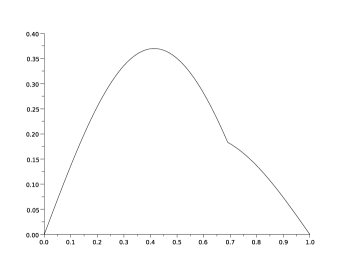
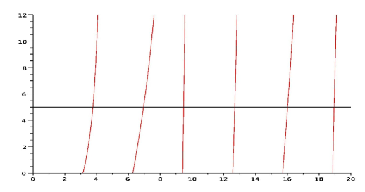
Figure 3: Left, the first eigenfunction of $A$, i.e. the fundamental mode of resonance of the flute with an open hole. Right, the graphic of the function $f_{a}$ and the intersections with the line $y=\alpha\delta$ giving the frequencies of the flute. The references values are $a=0.7$ and $\alpha\delta=5$.

Using the above computations, we can do several remarks about the resonances of the flute with a small open hole, as predicted by our model.

• The eigenfunctions of $A$ corresponds to the expected profile of the pressure in the flute with an open hole, see Figure 3 and the ones of [5], [7] and [26].

• The note of the flute corresponds to the fundamental frequency $\mu=\sqrt{\lambda^{1}}$. To obtain a given note, one can adjust both $\delta$ (the size of the hole) and $a$ (the place of the hole). This enables to place smartly the different holes to obtain some notes by combining the opening of several holes (fork fingering). We can also compute the change of frequency produced by only half opening the hole (half-holing). Notice that changing the shape of the hole affects the coefficient $\alpha$.

• The overtones of the flute correspond to the other frequencies $\mu=\sqrt{\lambda^{k}}$ with $k\geq 2$. We can see in Figure 3 that they are not exactly harmonic, i.e. they are not multiples of the fundamental frequency. This explains why the sound of flutes, which have only a small hole opened, is uneven and not as pure as the sound produced by a simple tube. In other words, our model directly explains the observation that the effective length approximation depends on the considered frequency. Moreover, when $\mu$ increases, the slope of $f_{a}$ becomes steeper due to the factor $\mu$ in (2.1) and the solutions of (2.1) are closer to $\mu=k\pi$. This is consistant with the observation that high frequencies are less affected by the presence of the hole than low frequencies, see [26] or [25]. However, notice that this is only roughly true since for example one can see on Figure 3 that the second overtone is almost equal to $3\pi$, whereas the fourth one is less close to $5\pi$. This comes from the fact that $a=0.7$ is almost a node of the mode $\sin(3\pi x)$.

• Of course, when $\delta=0$, we recover the equation $\sin\mu=0$ corresponding to the eigenvalue of the open tube without hole. When $\delta\rightarrow+\infty$, i.e. when the hole is very large, we recover the equations $\sin(\mu a)=0$ or $\sin(\mu(1-a))=0$, which correspond to two separated tubes of lengths $a$ and $1-a$ (in fact the part $(a,1)$ is not important because this is not the part of the tube which is excited by the fipple). When the hole is of intermediate size, the fundamental frequency corresponds to a tube of intermediate length $\tilde{a}\in(a,1)$, but the overtones are not the same as the ones of the tube of length $\tilde{a}$.

• The thin domain techniques used here are general and do not depend on the fact that the section of the tube $\Omega_{\varepsilon}$ is a square and not a disk. If the surface $g(x)$ of the section of the tube is not constant (think at the end of a clarinet), then the operator $\partial_{xx}^{2}$ in the definition of $A$ must be replaced by ${\small\frac{1}{g(x)}}\partial_{x}(g(x)\partial_{x}.)$, see [13]. Of course, if there are several open holes, then other terms of the type $\alpha\delta u(a)v(a)$ appear in (1.3).

To conclude, we obtain in this article a mathematical model for the flute with a small open hole, which consists in a one-dimensional operator different from a simple Laplacian operator. It yields simple explanation of some observations as the fact that the overtones are not harmonic.

3 Focusing on the hole: the rescaled problem

When $\varepsilon$ goes to zero, if one rescales the domain $\Omega_{\varepsilon}$ with a ratio $1/(\delta\varepsilon^{2})$ to focus on the hole, then one sees the rescaling domain $\Omega_{\varepsilon}$ converging to the half-space $x_{2}<0$ (see Figure 4). The purpose of this section is to introduce the technical background to be able study our problem in this rescaled frame. For the reader interested in more details about the Poisson problem in unbounded domain, we refer to [24].

Figure 4: The cube $K_{\varepsilon}$, part of the half-space $K=\{x\in\mathbb{R}^{3},~{}x_{2}<0\}$, and the corresponding boundaries. When $\varepsilon$ goes to $0$, the cube $K_{\varepsilon}$ converges to $K$, whereas the hole $\partial K(hole)$ remains unchanged.

3.1 The space $\dot{H}^{1}(K)$

Let $K$ be the half-space $\{x\in\mathbb{R}^{3},~{}x_{2}<0\}$. For any $\varepsilon>0$, we introduce the cube

$$K_{\varepsilon}=\left(\frac{-1}{2\delta\varepsilon},\frac{1}{2\delta\varepsilon}\right)\times\left(\frac{-1}{\delta\varepsilon},0\right)\times\left(\frac{-1}{2\delta\varepsilon},\frac{1}{2\delta\varepsilon}\right)$$

as shown in Figure 4. We denote by $\partial K_{\varepsilon}(hole)$ the part of the boundary $(-1/2,1/2)\times\{0\}\times(-1/2,1/2)$ corresponding to the hole. We denote $\partial K_{\varepsilon}(up)$ the remaining part of the upper face. We also denote by $\partial K(hole)$ and $\partial K(up)$ the corresponding parts of the boundary of the half-space $K$. See Figure 4.

We introduce the space $\dot{H}^{1}(K)$ defined by

$$\dot{H}^{1}(K)=\{v\in H^{1}_{loc}(K)~{},~{}\nabla v\in L^{2}(K)\text{ and }v=0\text{ on }\partial K(hole)\}~{}$$ (3.1)

and we equip it with the scalar product

$$\langle\varphi|\psi\rangle_{\dot{H}^{1}(K)}=\int_{K}\nabla\varphi.\nabla\psi~{}.$$ (3.2)

We also introduce the space $\dot{H}^{1}_{0}(K)$ which is the completion of

$$\mathcal{C}^{\infty}_{0}(\overline{K})=\{\varphi\in\mathcal{C}^{\infty}(\overline{K})~{}/~{}\mathrm{supp}(\varphi)\text{ is compact and }\varphi\equiv 0\text{ on }\partial K(hole)\}$$ (3.3)

with respect to the $\dot{H}^{1}$ scalar product defined in (3.2).

Let $\chi\in\mathcal{C}^{\infty}(\overline{K})$ be such that $\chi\equiv 1$ outside a compact set, $\chi\equiv 0$ on $\partial K(hole)$ and $\partial_{\nu}\chi\equiv 0$ on $\partial K(up)$. Following [24], we get the following results.

Theorem 3.1.

The spaces $\dot{H}^{1}(K)$ and $\dot{H}^{1}_{0}(K)$ equipped with the scalar product (3.2) are Hilbert spaces and

$$\dot{H}^{1}(K)=\dot{H}^{1}_{0}(K)\oplus\mathbb{R}\chi~{},$$ (3.4)

this sum being a direct sum of closed subspaces.

Moreover, a function $u\in\dot{H}^{1}(K)$ belongs to $\dot{H}^{1}_{0}(K)$ if and only if it belongs to $L^{6}(K)$. As a consequence, the splitting of $u\in\dot{H}^{1}(K)$ given by (3.4) is uniquely determined by $u=\dot{u}+\overline{u}\chi$, where

$$\overline{u}=\lim_{\varepsilon\rightarrow 0}\frac{1}{|K_{\varepsilon}|}\int_{K_{\varepsilon}}u(x)dx$$

is the average of $u$, which is well defined.

Proof : The direct sum (3.4) is a particular case of Theorem 2.15 of [24]. The equivalence between $u\in\dot{H}^{1}_{0}(K)$ and $u\in L^{6}(K)$ is given by Theorem 2.8 of [24]. Let $u=\dot{u}+c\chi$ with $\dot{u}\in\dot{H}^{1}_{0}(K)$ and $c\in\mathbb{R}$. Since $\dot{u}\in L^{6}(K)$, we have $\int_{K_{\varepsilon}}|\dot{u}|\leq C|K_{\varepsilon}|^{5/6}$ and thus the average of $\dot{u}$ is well defined and equal to $0$. Since the average of $\chi$ is well defined and equal to $1$, the average of $u$ is also well defined and it is equal to $c$. $\square$

3.2 The function $\zeta$

We now introduce the function $\zeta$, which is used to define the coefficient $\alpha$ in (1.1).

Proposition 3.2.

There is a unique weak solution $\zeta$ of

$$\left\{\begin{array}[]{ll}\Delta\zeta=0&\text{ on }K\\ \zeta=0&\text{ on }\partial K(hole)\\ \partial_{\nu}\zeta=0&\text{ on }\partial K(up)\\ \overline{\zeta}=1&\end{array}\right.$$ (3.5)

in the sense that $\zeta\in\dot{H}^{1}(K)$, $\overline{\zeta}=1$ and

$$\forall\varphi\in\mathcal{C}^{\infty}_{0}(K)~{},~{}~{}\int_{K}\nabla\zeta.\nabla\varphi=0~{}.$$

Proof : Theorem 3.1 shows that $\zeta=\chi+\dot{\zeta}$ with $\dot{\zeta}\in\dot{H}^{1}_{0}(K)$. Then, Proposition 3.2 is a direct application of Lax-Milgram Theorem to the variational equation

$$\forall\dot{\varphi}\in\dot{H}^{1}_{0}(K)~{},~{}~{}\int_{K}\nabla\dot{\zeta}\nabla\dot{\varphi}=-\int_{K}\Delta\chi.\dot{\varphi}~{}.$$

See [24] for a discussion on this kind of variational problems. $\square$

The function $\zeta$ yields a different way to write the scalar product in $\dot{H}^{1}(K)$.

Proposition 3.3.

The function $\zeta$ is the orthogonal projection of $\chi$ on the orthogonal space of $\dot{H}^{1}_{0}(K)$ in $\dot{H}^{1}(K)$.

Thus, for all $u$ and $v$ in $\dot{H}^{1}(K)$, there exist two unique functions $\dot{u}$ and $\dot{v}$ in $\dot{H}^{1}_{0}(K)$ such that $u=\dot{u}+\overline{u}\zeta$ and $v=\dot{v}+\overline{v}\zeta$. Moreover,

$$\langle u|v\rangle_{\dot{H}^{1}(K)}~{}=~{}\int_{K}\nabla\dot{u}(x).\nabla\dot{v}(x)~{}dx~{}+~{}\alpha\overline{u}.\overline{v}~{},$$

where $\alpha$ is defined by (1.1).

3.3 Weak $K_{\varepsilon}-$convergence

As one can see in Figure 4, if $(u_{\varepsilon})$ is a sequence of functions defined in $\Omega_{\varepsilon}$, then the rescaled functions $w_{\varepsilon}$ are only defined in the box $K_{\varepsilon}$ and not in the whole space $K$. Hence, we have to introduce a suitable notion of weak convergence.

Proposition 3.4.

Let $(w_{\varepsilon})_{\varepsilon>0}$ be a sequence of functions of $H^{1}(K_{\varepsilon})$ vanishing on $\partial K_{\varepsilon}(hole)$. Assume that

$$\exists C>0~{},~{}~{}\forall\varepsilon>0~{},~{}~{}\int_{K_{\varepsilon}}|\nabla w_{\varepsilon}|^{2}\leq C~{}.$$

Then, there exists a subsequence $(w_{\varepsilon_{n}})_{n\in\mathbb{N}}$, with $\varepsilon_{n}\rightarrow 0$, which converges weakly to a function $w_{0}\in\dot{H}^{1}(K)$ in the sense that

$$\forall\varphi\in\dot{H}^{1}(K)~{},~{}~{}\int_{K_{\varepsilon_{n}}}\nabla w_{\varepsilon_{n}}\nabla\varphi\xrightarrow[~{}~{}\varepsilon_{n}\longrightarrow 0~{}~{}]{}\int_{K}\nabla w_{0}\nabla\varphi~{}.$$

Moreover, the average of $w_{0}$ is given by

$$\overline{w}_{0}=\lim_{\varepsilon_{n}\rightarrow 0}\frac{1}{|K_{\varepsilon_{n}}|}\int_{K_{\varepsilon_{n}}}w_{\varepsilon}~{}.$$ (3.6)

Before starting to prove Proposition 3.4, we recall Poincaré-Wirtinger inequality.

Lemma 3.5.

(Poincaré-Wirtinger inequality)
There exists a constant $C>0$ such that, for any $\varepsilon>0$ and any function $\varphi\in H^{1}(K_{\varepsilon})$,

$$\int_{K_{\varepsilon}}\left|\varphi(x)-\frac{1}{|K_{\varepsilon}|}\int_{K_{\varepsilon}}\varphi(s)ds\right|^{6}dx\leq C\left(\int_{K_{\varepsilon}}|\nabla\varphi(x)|^{2}dx\right)^{3}~{}.$$ (3.7)

Proof : First, let us set $\varepsilon=1$. The classical Poincaré inequality (see [10] for example) states that

$$\int_{K_{1}}\left|\varphi(x)-\frac{1}{|K_{1}|}\int_{K_{1}}\varphi(s)ds\right|^{2}dx\leq C\int_{K_{1}}|\nabla\varphi(x)|^{2}dx~{}.$$

Thus, the right-hand side controls the $H^{1}-$norm of $\varphi-\overline{\varphi}$. Then, the Sobolev inequalities shows that (3.7) holds for $\varepsilon=1$. Now, the crucial point is to notice that the constant $C$ in (3.7) is independent of the size of the cube $K_{\varepsilon}$ since both sides of the inequality behave similarly with respect to scaling. $\square$

Proof of Proposition 3.4 : First notice that $\dot{H}^{1}_{0}(K)$ is separable due to the density of $\mathcal{C}^{\infty}_{0}-$functions. Hence, $\dot{H}^{1}(K)$ is also separable and by a diagonal extraction argument, we can extract a subsequence $\varepsilon_{n}\rightarrow 0$ such that for all $\varphi\in\dot{H}^{1}(K)$, $\int_{K_{\varepsilon_{n}}}\nabla w_{\varepsilon_{n}}\nabla\varphi$ converges to a limit $L(\varphi)$ with $L(\varphi)\leq C\|\varphi\|_{\dot{H}^{1}}$. By Riesz representation Theorem, there exists $w_{0}\in\dot{H}^{1}(K)$ such that $L(\varphi)=\langle w_{0}|\varphi\rangle$.

To prove (3.6), we follow the arguments of [18]. We set $\overline{w}_{\varepsilon}=\frac{1}{|K_{\varepsilon}|}\int_{K_{\varepsilon}}w_{\varepsilon}$. Let $p\in\mathbb{N}$. Lemma 3.5 and the fact that $\int_{K_{\varepsilon}}|\nabla w_{\varepsilon}|^{2}$ is bounded, show that there exists a constant $C$ independent of $\varepsilon$ such that $\int_{K_{\varepsilon}}|w_{\varepsilon}(x)-\overline{w}_{\varepsilon}|^{6}dx\leq C$. Thus,

$$\forall\varepsilon<\frac{1}{p}~{},~{}~{}\int_{K_{1/p}}|w_{\varepsilon}(x)-\overline{w}_{\varepsilon}|^{6}dx\leq C~{}.$$ (3.8)

By Sobolev inequality, we know that $w_{\varepsilon}$ is bounded in $L^{6}(K_{1/p})$ (remember that $w_{\varepsilon}$ vanishes on $\partial K_{1/p}(hole)$). Thus $\overline{w}_{\varepsilon}$ is bounded and up to extracting another subsequence, we can assume that $\overline{w}_{\varepsilon_{n}}$ converges to some limit $\beta\in\mathbb{R}$. By a diagonal extraction argument, we can also assume that $w_{\varepsilon_{n}}$ converges to $w_{0}$ weakly in $L^{6}(K_{1/p})$, for any $p\in\mathbb{N}$. As a consequence, (3.8) implies that

$$\int_{K_{1/p}}|w_{0}(x)-\beta|^{6}dx\leq\limsup_{\varepsilon\longrightarrow 0}\int_{K_{1/p}}|w_{\varepsilon}(x)-\overline{w}_{\varepsilon}|^{6}dx\leq C~{}.$$

Since the previous estimate is uniform with respect to $p\in\mathbb{N}$ and since $K_{1/p}$ grows to $K$ when $p$ goes to $+\infty$, we obtain that $w_{0}-\beta$ belongs to $L^{6}(K)$ and thus $w_{0}-\beta\chi\in L^{6}(K)$. Theorem 3.1 shows that $w_{0}-\beta\chi$ belongs to $\dot{H}^{1}_{0}(K)$ i.e. $\beta=\overline{w}_{0}$. $\square$

4 Lower-semicontinuity of the spectrum

This section is devoted to the following result.

Proposition 4.1.

$$\forall k\in\mathbb{N}^{*}~{},~{}~{}0\leq\displaystyle\limsup_{\varepsilon\rightarrow 0}\lambda^{k}_{\varepsilon}\leq\lambda^{k}~{}.$$

Proof : Let $(u^{k})$ be a sequence of eigenfunctions of $A$ corresponding to the eigenvalues $\lambda^{k}$. Since $A$ is symmetric, we may assume that $\langle u^{k}|u^{j}\rangle_{L^{2}(0,1)}=0$ for $k\neq j$. The main idea of the proof of Proposition 4.1 is to construct an embedding $I_{\varepsilon}:H^{1}_{0}(0,1)\rightarrow H^{1}_{0}(\Omega_{\varepsilon})$ such that the functions $I_{\varepsilon}u^{k}$ are almost $L^{2}-$orthogonal and such that

$$\frac{\int_{\Omega_{\varepsilon}}|\nabla I_{\varepsilon}u^{k}|^{2}}{\int_{\Omega_{\varepsilon}}|I_{\varepsilon}u^{k}|^{2}}\xrightarrow[~{}~{}~{}\varepsilon\longrightarrow 0~{}~{}~{}]{}\lambda^{k}~{}.$$ (4.1)

The definition of the embedding $I_{\varepsilon}:H^{1}_{0}(0,1)\rightarrow H^{1}_{0}(\Omega_{\varepsilon})$ is as follows.

Far from the hole: we split the functions $u^{k}$ into two parts $u^{k}_{|(0,a)}$ and $u^{k}_{|(a,1)}$, we slightly rescale them so that they are defined in $(\varepsilon,a-\varepsilon/2)$ and $(a+\varepsilon/2,1)$ respectively, and we embed both parts in $L^{2}(\Omega_{\varepsilon})$ by setting

$$\varphi_{\varepsilon}^{k}(x)=u^{k}\left(\frac{a}{a-3\varepsilon/2}(x_{1}-\varepsilon)\right)~{}~{}\text{ and }~{}~{}\psi_{\varepsilon}^{k}(x)=u^{k}\left(a+\frac{1-a}{1-a-\varepsilon/2}(x_{1}-a-\varepsilon/2)\right)~{}.$$

Near the hole: let $\zeta\in\dot{H}^{1}(K)$ be as in Proposition 3.2 and let $\zeta=\dot{\zeta}+\chi$ be the splitting given by Theorem 3.1 (where we use that $\overline{\zeta}=1$ by definition). By the definition of $\dot{H}^{1}_{0}(K)$, there exists a sequence of functions $(\dot{\zeta}_{\varepsilon})\in\mathcal{C}^{\infty}_{0}(K)$ converging to $\dot{\zeta}$ in $\dot{H}^{1}_{0}(K)$. Therefore, there exists a sequence $\zeta_{\varepsilon}=\dot{\zeta}_{\varepsilon}+\chi\in\mathcal{C}^{\infty}(K)\cap\dot{H}^{1}(K)$ such that $\zeta_{\varepsilon}\equiv 1$ outside a compact set and $(\zeta_{\varepsilon})$ converges strongly to $\zeta$ when $\varepsilon$ goes to zero. Notice that we may assume that $\zeta_{\varepsilon}\equiv 1$ outside a compact set of the cube $K_{\varepsilon}$ defined in Section 3. We set $\tilde{\zeta}_{\varepsilon}(x)=\zeta_{\varepsilon}((x-(a,0,0))/(\delta\varepsilon^{2}))$ and $I_{\varepsilon}u^{k}=u^{k}(a)\tilde{\zeta}_{\varepsilon}$ in the cube $B_{\varepsilon}=(a,0,0)+\delta\varepsilon^{2}K_{\varepsilon}$.

Summarizing: the whole embedding $I_{\varepsilon}$ is described by Figure 5.

Figure 5: The embedding $u^{k}_{\varepsilon}=I_{\varepsilon}u^{k}$ of $u^{k}\in H^{1}_{0}(0,1)$ into $H^{1}_{0}(\Omega_{\varepsilon})$ (lateral view).

Calculing the scalar products: by change of variables, we have

$$\int_{B_{\varepsilon}}|\tilde{\zeta}_{\varepsilon}|^{2}=\delta^{3}\varepsilon^{6}\int_{K_{\varepsilon}}|\zeta_{\varepsilon}|^{2}\leq\delta^{3}\varepsilon^{6}\left(\left(\int_{K_{\varepsilon}}|\dot{\zeta}_{\varepsilon}|^{2}\right)^{1/2}+\left(\int_{K_{\varepsilon}}|\chi|^{2}\right)^{1/2}\right)^{2}~{}.$$

Since $\chi$ is a bounded $\mathcal{C}^{\infty}$ function and since the volume of $K_{\varepsilon}$ is of order $1/\varepsilon^{3}$, we have $\int_{K_{\varepsilon}}|\chi|^{2}=O(1/\varepsilon^{3})$. Due to Theorem 3.1, $\dot{\zeta}_{\varepsilon}$ converges to $\dot{\zeta}$ in $L^{6}(K)$ and thus

$$\int_{K_{\varepsilon}}|\dot{\zeta}_{\varepsilon}|^{2}\leq\left(\int_{K_{\varepsilon}}|\dot{\zeta}_{\varepsilon}|^{6}\right)^{1/3}\left(\int_{K_{\varepsilon}}1\right)^{2/3}=O(1/\varepsilon^{2})~{}.$$

Therefore, we get that $\int_{B_{\varepsilon}}|\tilde{\zeta}_{\varepsilon}|^{2}=O(\varepsilon^{3})$. Thus, the $L^{2}-$norm of $u^{k}_{\varepsilon}=I_{\varepsilon}u^{k}$ is mostly due to the $L^{2}-$norms of $\varphi_{\varepsilon}^{k}$ and $\psi_{\varepsilon}^{k}$ and so, for any $k$ and $j$,

$$\langle u_{\varepsilon}^{k}|u_{\varepsilon}^{j}\rangle_{L^{2}(\Omega_{\varepsilon})}=\varepsilon^{2}\langle u^{k}|u^{j}\rangle_{L^{2}(0,1)}+o(\varepsilon^{2})~{}.$$ (4.2)

On the other hand, we have $\int_{B_{\varepsilon}}|\nabla\tilde{\zeta}_{\varepsilon}|^{2}=\delta\varepsilon^{2}\int_{K_{\varepsilon}}|\nabla\zeta_{\varepsilon}|^{2}$. Since $(\zeta_{\varepsilon})$ converges to $\zeta$ in $\dot{H}^{1}(K)$ and due to the definition (1.1) of $\alpha$, $\int_{K_{\varepsilon}}|\nabla\zeta_{\varepsilon}|^{2}$ converges to $\alpha$. Therefore, for any $k$ and $j$,

$$\int_{\Omega_{\varepsilon}}\nabla u_{\varepsilon}^{k}\nabla u_{\varepsilon}^{j} =\int_{\Omega_{\varepsilon}}\nabla\varphi_{\varepsilon}^{k}\nabla\varphi_{\varepsilon}^{j}+\int_{\Omega_{\varepsilon}}\nabla\psi_{\varepsilon}^{k}\nabla\psi_{\varepsilon}^{j}+u^{k}(a)u^{j}(a)\int_{B_{\varepsilon}}|\nabla\tilde{\zeta}_{\varepsilon}|^{2}$$

$$=\varepsilon^{2}\left(\int_{0}^{a}\partial_{x}u^{k}(x)\partial_{x}u^{j}(x)dx+\int_{a}^{1}\partial_{x}u^{k}(x)\partial_{x}u^{j}(x)dx\right.$$

$$~{}~{}~{}~{}~{}~{}~{}~{}~{}~{}~{}~{}~{}+\left.\delta u^{k}(a)u^{j}(a)\int_{K_{\varepsilon}}|\nabla\zeta_{\varepsilon}|^{2}\right)+o(\varepsilon^{2})~{}$$

$$=\varepsilon^{2}\left(\int_{0}^{1}\partial_{x}u^{k}(x)\partial_{x}u^{j}(x)dx+\alpha\delta u^{k}(a)u^{j}(a)\right)+o(\varepsilon^{2})~{}$$

$$=\varepsilon^{2}\langle Au^{k}|u^{j}\rangle_{L^{2}}+o(\varepsilon^{2})~{}.$$ (4.3)

Hence the previous estimates yield the limit (4.1).

Applying the Min-Max formula: for $\varepsilon$ small enough, (4.2) implies that the functions $u_{\varepsilon}^{k}$ are linearly independent. Due to the Min-Max Principle (see [21] for example), we know that

$$\lambda^{k}_{\varepsilon}~{}\leq~{}\min_{p_{1}<p_{2}<\ldots<p_{k}}~{}\max_{c\in\mathbb{R}^{k}_{*}}~{}\frac{\int_{\Omega_{\varepsilon}}|\sum_{i=1}^{k}c_{i}\nabla I_{\varepsilon}u^{p_{i}}|^{2}}{\int_{\Omega_{\varepsilon}}|\sum_{i=1}^{k}c_{i}I_{\varepsilon}u^{p_{i}}|^{2}}~{}.$$ (4.4)

The above estimates (4.2) and (4.3) show that, for any $c\in\mathbb{R}^{k}_{*}$, we have

$$\frac{\int_{\Omega_{\varepsilon}}|\sum_{i=1}^{k}c_{i}\nabla I_{\varepsilon}u^{p_{i}}|^{2}}{\int_{\Omega_{\varepsilon}}|\sum_{i=1}^{k}c_{i}I_{\varepsilon}u^{p_{i}}|^{2}}=\frac{\langle A\sum_{i=1}^{k}c_{i}u^{p_{i}}|\sum_{i=1}^{k}c_{i}u^{p_{i}}\rangle_{L^{2}}}{\|\sum_{i=1}^{k}c_{i}u^{p_{i}}\|_{L^{2}}^{2}}+o(1)~{},$$

where the remainder $o(1)$ is uniform with respect to $c$ when $\varepsilon$ goes to zero. Using the Min-Max Principle another time, we get

$$\min_{p_{1}<p_{2}<\ldots<p_{k}}~{}\max_{c\in\mathbb{R}^{k}_{*}}~{}\frac{\int_{\Omega_{\varepsilon}}|\sum_{i=1}^{k}c_{i}\nabla I_{\varepsilon}u^{p_{i}}|^{2}}{\int_{\Omega_{\varepsilon}}|\sum_{i=1}^{k}c_{i}I_{\varepsilon}u^{p_{i}}|^{2}}=\lambda^{k}+o(1)~{}.$$

This finishes the proof of Proposition 4.1. $\square$

5 Upper-semicontinuity of the spectrum

Let $\varepsilon>0$ and let $(u^{k}_{\varepsilon})$ be a sequence of eigenfunctions of $\Delta_{\varepsilon}$ corresponding to the eigenvalues $(\lambda_{\varepsilon}^{k})$. We can assume that the functions $u^{k}_{\varepsilon}$ are orthogonal in $L^{2}(\Omega_{\varepsilon})$ and that $\|u^{k}_{\varepsilon}\|_{L^{2}}=\varepsilon$. To work on a fixed domain, we set $\Omega=(0,1)^{3}$ and we introduce the functions $v^{k}_{\varepsilon}=Ju^{k}_{\varepsilon}$ where $J$ is the canonical embedding of $H^{1}(\Omega_{\varepsilon})$ into $H^{1}(\Omega)$, that is that

$$Ju^{k}_{\varepsilon}(y)=v^{k}_{\varepsilon}(y)=v^{k}_{\varepsilon}(y_{1},\tilde{y})=u^{k}_{\varepsilon}(y_{1},\varepsilon\tilde{y})~{}.$$

We have

$$-\left(\partial^{2}_{y_{1}y_{1}}+\frac{1}{\varepsilon^{2}}\partial^{2}_{\tilde{y}\tilde{y}}\right)v^{k}_{\varepsilon}=\lambda^{k}_{\varepsilon}v^{k}_{\varepsilon}~{}~{}\text{ and }~{}~{}\|v^{k}_{\varepsilon}\|_{L^{2}}=1~{}.$$

By multiplying the previous equation by $v^{k}_{\varepsilon}$ and integrating, we get

$$\int_{\Omega}|\partial_{y_{1}}v^{k}_{\varepsilon}|^{2}+\frac{1}{\varepsilon^{2}}|\partial_{\tilde{y}}v^{k}_{\varepsilon}|^{2}=\lambda^{k}_{\varepsilon}~{}.$$ (5.1)

Proposition 4.1 shows that $(\lambda^{k}_{\varepsilon})_{\varepsilon>0}$ is bounded. Therefore, up to extracting a subsequence, we may assume that $(\lambda^{k}_{\varepsilon})$ converges to $\lambda^{k}_{0}=\liminf_{\varepsilon\rightarrow 0}\lambda^{k}_{\varepsilon}$ when $\varepsilon$ goes to $0$ and that $(v^{k}_{\varepsilon})$ converges to a function $v^{k}_{0}\in H^{1}(\Omega)$, strongly in $H^{3/4}(\Omega)$ and weakly in $H^{1}(\Omega)$. Moreover, (5.1) shows that $v^{k}_{0}$ depends only on $y_{1}$. In the following, we will abusively denote by $v^{k}_{0}$, either the function in $H^{1}(\Omega)$ or the one-dimensional function in $H^{1}(0,1)$.

The purpose of this section is to use the methods of [18] (see also [16] and [17]) to prove the following result.

Proposition 5.1.

For all $k\in\mathbb{N}^{*}$, the function $v^{k}_{0}$ is an eigenfunction of $A$ for the eigenvalue $\lambda^{k}_{0}$.

Proposition 5.1 finishes the proof of Theorem 1.1 since we immediately get the upper-semicontinuity of the spectrum.

Corollary 5.2.

$$\forall k\in\mathbb{N}^{*}~{},~{}~{}\displaystyle\liminf_{\varepsilon\rightarrow 0}\lambda^{k}_{\varepsilon}\geq\lambda^{k}~{}.$$

Proof : We recall that the functions $v^{k}_{\varepsilon}$ are orthonormalised in $L^{2}(\Omega)$ and converge strongly in $L^{2}(\Omega)$ to $v^{k}_{0}$. Thus, the functions $v^{k}_{0}$ are also orthonormalised. Since $\lambda^{k}_{0}=\liminf_{\varepsilon\rightarrow 0}\lambda^{k}_{\varepsilon}$, we know that $\lambda^{1}_{0}\leq\lambda^{2}_{0}\leq\ldots\leq\lambda^{k}_{0}$. Then, Proposition 5.1 shows that $\lambda^{1}_{0}$, $\ldots$, $\lambda^{k}_{0}$ are $k$ eigenvalues of $A$ with linearly independent eigenfunctions, and thus that the largest one $\lambda^{k}_{0}$ is larger than $\lambda^{k}$. $\square$

The proof of Proposition 5.1 splits into several lemmas. To simplify the notations, we will omit the exponent $k$ in the remaining part of this section and we will write $u_{\varepsilon}$ for $u_{\varepsilon}^{k}$, $v_{\varepsilon}$ for $v_{\varepsilon}^{k}$ etc.

Lemma 5.3.

Let $B_{\varepsilon}\subset\Omega_{\varepsilon}$ be any cube of size $\varepsilon$ and let $\Gamma_{\varepsilon}$ be one of its faces. Then,

$$\frac{1}{\varepsilon^{3}}\int_{B_{\varepsilon}}u_{\varepsilon}(x)dx=\frac{1}{\varepsilon^{2}}\int_{\Gamma_{\varepsilon}}u_{\varepsilon}(\tilde{x})d\tilde{x}+o(1)~{}.$$ (5.2)

As a consequence, $v_{0}$ satisfies both Dirichlet boundary conditions $v_{0}(0)=v_{0}(1)=0$.

Proof : We split the cube in slices $B_{\varepsilon}=\cup_{s\in[0,\varepsilon]}\Gamma_{\varepsilon}(s)$ with $\Gamma_{\varepsilon}=\Gamma_{\varepsilon}(0)$ and we set $x=(s,\tilde{x})$ with $\tilde{x}\in\Gamma_{\varepsilon}(s)$. For each $s$, we have

$$\left|\int_{\Gamma_{\varepsilon}(s)}u_{\varepsilon}(s,\tilde{x})d\tilde{x}-\int_{\Gamma_{\varepsilon}(0)}u_{\varepsilon}(0,\tilde{x})d\tilde{x}\right| \leq\int_{\Gamma_{\varepsilon}(\xi)}\int_{0}^{s}\left|\nabla u_{\varepsilon}(\xi,\tilde{x})\right|d\xi d\tilde{x}$$

$$\leq\varepsilon\sqrt{s}\sqrt{\int_{\Gamma_{\varepsilon}(\xi)}\int_{0}^{s}\left|\nabla u_{\varepsilon}(\xi,\tilde{x})\right|^{2}d\xi d\tilde{x}}~{}.$$

To show (5.2), we integrate the above inequality from $s=0$ to $s=\varepsilon$ and we notice that $\|\nabla u_{\varepsilon}\|_{L^{2}}=\lambda_{\varepsilon}\|u_{\varepsilon}\|_{L^{2}}=\lambda_{\varepsilon}\varepsilon=\mathcal{O}(\varepsilon)$.

The fact that $v_{0}(1)=0$ follows from $v_{\varepsilon}(1,\tilde{x})=0$ and the strong convergence of $v_{\varepsilon}$ to $v_{0}$ in $H^{3/4}(\Omega)$. To obtain the other Dirichlet boundary condition, we apply (5.2) to the cube $B_{\varepsilon}=[0,\varepsilon]\times[-\varepsilon,0]\times[-\varepsilon/2,\varepsilon/2]$ at the left-end of $\Omega_{\varepsilon}$. Since $u_{\varepsilon}$ vanishes on the upper face of $B_{\varepsilon}$, the average of $u_{\varepsilon}$ goes to zero in $B_{\varepsilon}$. Applying (5.2) again, the average of $u_{\varepsilon}$ goes to zero on the left face of $B_{\varepsilon}$. Thus, the average of $v_{\varepsilon}$ goes to zero on the left face $\Gamma=\{0\}\times[-1,0]\times[-1/2,1/2]$ of $\Omega$ and hence $\int_{\Gamma}v_{0}(0,\tilde{y})d\tilde{y}=0$ because $v_{\varepsilon}$ converges to $v_{0}$ in $H^{3/4}(\Omega)$. Since $v_{0}$ does not depend on $\tilde{y}$, this yields $v_{0}(0)=0$. $\square$

We now focus on what happens close to the hole at $(a,0,0)$. To this end, we use the notations of Section 3 and we introduce the functions $w_{\varepsilon}\in H^{1}(K_{\varepsilon})$ defined by

$$\forall x\in K_{\varepsilon}~{},~{}~{}w_{\varepsilon}(x)=u_{\varepsilon}((a,0,0)+\delta\varepsilon^{2}x)~{}.$$

The functions $w_{\varepsilon}$ will be useful to study the behaviour of $u_{\varepsilon}$ in the cube

$$B_{\varepsilon}=(a-\varepsilon/2,a+\varepsilon/2)\times(-\varepsilon,0)\times(-\varepsilon/2,\varepsilon/2)~{}.$$

We show that they weakly converges to $v_{0}(a)\zeta$ in $\dot{H}^{1}(K)$ in the following sense.

Lemma 5.4.

For all $\varphi\in\dot{H}^{1}(K)$,

$$\int_{K_{\varepsilon}}\nabla w_{\varepsilon}\nabla\varphi\xrightarrow[~{}~{}\varepsilon\longrightarrow 0~{}~{}]{}v_{0}(a)\int_{K}\nabla\zeta\nabla\varphi~{}.$$

Proof : We have

$$\int_{K_{\varepsilon}}|\nabla w_{\varepsilon}|^{2}=\frac{1}{\delta\varepsilon^{2}}\int_{B_{\varepsilon}}|\nabla u_{\varepsilon}|^{2}\leq\frac{1}{\delta\varepsilon^{2}}\int_{\Omega_{\varepsilon}}|\nabla u_{\varepsilon}|^{2}=\frac{1}{\delta\varepsilon^{2}}\lambda_{\varepsilon}\int_{\Omega_{\varepsilon}}|u_{\varepsilon}|^{2}=\frac{\lambda_{\varepsilon}}{\delta}~{}.$$

Moreover, the average of $w_{\varepsilon}$ in $K_{\varepsilon}$ is equal to the one of $u_{\varepsilon}$ in $B_{\varepsilon}$, which converges to $v_{0}(a)$ due to Lemma 5.3 and the convergence of $v_{\varepsilon}$ to $v_{0}$ in $H^{3/4}(\Omega)$. Applying Proposition 3.4, we obtain the weak convergence of a subsequence of $w_{\varepsilon}$ to a limit $w_{0}$, whose average is $\overline{w}_{0}=v_{0}(a)$. To prove Lemma 5.4, it remains to show that $w_{0}=v_{0}(a)\zeta$, which does not depend on the chosen subsequence $(\varepsilon_{n})$.

Let $\varphi\in\mathcal{C}^{\infty}_{0}(K)$ and assume that $\varepsilon$ is small enough such that $\mathrm{supp}(\varphi)\subset K_{\varepsilon}$. We set

$$\forall x\in B_{\varepsilon}~{},~{}~{}\tilde{\varphi}_{\varepsilon}(x)=\varphi\left(\frac{x-(a,0,0)}{\delta\varepsilon^{2}}\right)$$

and we extend $\tilde{\varphi}_{\varepsilon}$ by zero in $\Omega_{\varepsilon}$. Since

$$\|u_{\varepsilon}\|_{L^{2}}=\varepsilon~{}\text{ and }~{}\|\tilde{\varphi}_{\varepsilon}\|_{L^{2}(\Omega_{\varepsilon})}=\delta^{3/2}\varepsilon^{3}\|\varphi\|_{L^{2}(K)}~{},$$

we get

$$\int_{K_{\varepsilon}}\nabla w_{\varepsilon}\nabla\varphi=\frac{1}{\delta\varepsilon^{2}}\int_{B_{\varepsilon}}\nabla u_{\varepsilon}\nabla\tilde{\varphi}_{\varepsilon}=\frac{1}{\delta\varepsilon^{2}}\int_{\Omega_{\varepsilon}}\Delta u_{\varepsilon}\tilde{\varphi}_{\varepsilon}=\frac{\lambda_{\varepsilon}}{\delta\varepsilon^{2}}\int_{\Omega_{\varepsilon}}u_{\varepsilon}\tilde{\varphi}_{\varepsilon}\xrightarrow[~{}~{}\varepsilon\longrightarrow 0~{}~{}]{}0~{}.$$

Thus, $w_{0}$ is orthogonal to $\mathcal{C}^{\infty}_{0}(K)$ and hence to $\dot{H}^{1}_{0}(K)$ and Proposition 3.3 implies that $w_{0}=\overline{w}_{0}\zeta$. Since we already know that $\overline{w}_{0}=v_{0}(a)$, Lemma 5.4 is proved. $\square$

Proof of Proposition 5.1 : We have shown in Lemma 5.3 that $v_{0}$ satisfies Dirichlet boundary condition at $x_{1}=0$ and $x_{1}=1$. Let $\phi\in H^{1}_{0}(0,1)$ be a test function. We also denote by $\phi$ the canonical embedding of $\phi$ into $H^{1}(\Omega)$. We embed $\phi$ into $\Omega_{\varepsilon}$ by setting $\phi_{\varepsilon}=I_{\varepsilon}\phi$, where $I_{\varepsilon}$ is the embedding introduced in the proof of Proposition 4.1. Using the notations of Figure 5, we have

$$\int_{\Omega_{\varepsilon}}\nabla u_{\varepsilon}\nabla\phi_{\varepsilon}=\int_{x_{1}<a-\varepsilon/2}\nabla u_{\varepsilon}\nabla\varphi_{\varepsilon}+\phi(a)\int_{B_{\varepsilon}}\nabla u_{\varepsilon}\nabla\tilde{\zeta}_{\varepsilon}+\int_{x_{1}>a+\varepsilon/2}\nabla u_{\varepsilon}\nabla\psi_{\varepsilon}$$ (5.3)

The limits of the different terms are as follows. First, notice that

$$\int_{\Omega_{\varepsilon}}\nabla u_{\varepsilon}\nabla\phi_{\varepsilon}=\lambda_{\varepsilon}\int_{\Omega_{\varepsilon}}u_{\varepsilon}\phi_{\varepsilon}=\varepsilon^{2}\lambda_{\varepsilon}\int_{\Omega}v_{\varepsilon}J\phi_{\varepsilon}$$

where $J\phi_{\varepsilon}$ is the canonical embedding of $\phi_{\varepsilon}$ in $H^{1}(\Omega)$. Obviously, $J\phi_{\varepsilon}$ converges to $J\phi$ in $L^{2}(\Omega)$ and we know that $v_{\varepsilon}$ converges to $v_{0}$ in $L^{2}(\Omega)$. Thus,

$$\int_{\Omega_{\varepsilon}}\nabla u_{\varepsilon}\nabla\phi_{\varepsilon}=\varepsilon^{2}\lambda_{0}\int_{\Omega}v_{0}\phi+o(\varepsilon^{2})=\varepsilon^{2}\lambda_{0}\int_{0}^{1}v_{0}\phi+o(\varepsilon^{2})~{}.$$

In the parts $x_{1}<a-\varepsilon/2$ and $x_{1}>a+\varepsilon/2$, we know that $v_{\varepsilon}$ converges to $v_{0}$ weakly in $H^{1}(\Omega)$ and obviously $J\varphi_{\varepsilon}$ and $J\psi_{\varepsilon}$ converge to $\phi$ strongly in $H^{1}$. Moreover, notice that $J\varphi_{\varepsilon}$ and $J\psi_{\varepsilon}$ only depends on $x_{1}$. Hence,

$$\int_{x_{1}<a-\varepsilon/2}\nabla u_{\varepsilon}\nabla\varphi_{\varepsilon} +\int_{x_{1}>a+\varepsilon/2}\nabla u_{\varepsilon}\nabla\psi_{\varepsilon}$$

$$=\varepsilon^{2}\left(\int_{x_{1}<a-\varepsilon/2}\partial_{x_{1}}v_{\varepsilon}\partial_{x_{1}}(J\varphi_{\varepsilon})+\int_{x_{1}>a+\varepsilon/2}\partial_{x_{1}}v_{\varepsilon}\partial_{x_{1}}(J\psi_{\varepsilon})\right)$$

$$=\varepsilon^{2}\left(\int_{0}^{a}\partial_{x_{1}}v_{0}\partial_{x_{1}}\phi+\int_{a}^{1}\partial_{x_{1}}v_{0}\partial_{x_{1}}\phi\right)+o(\varepsilon^{2})~{}.$$

$$=\varepsilon^{2}\int_{0}^{1}\partial_{x_{1}}v_{0}\partial_{x_{1}}\phi+o(\varepsilon^{2})~{}.$$

The term of (5.3) in the box $B_{\varepsilon}$ is more delicate, but all the work has already been done in Lemma 5.4. Indeed we have

$$\int_{B_{\varepsilon}}\nabla u_{\varepsilon}\nabla\tilde{\zeta}_{\varepsilon}=\delta\varepsilon^{2}\int_{K_{\varepsilon}}\nabla w_{\varepsilon}\nabla\zeta_{\varepsilon}~{}.$$

By definition $\zeta_{\varepsilon}$ converges to $\zeta$ strongly in $\dot{H}^{1}(K)$. Thus, Lemma 5.4 implies that

$$\int_{B_{\varepsilon}}\nabla u_{\varepsilon}\nabla\tilde{\zeta}_{\varepsilon}=\delta\varepsilon^{2}v_{0}(a)\int_{K}\nabla\zeta\nabla\zeta+o(\varepsilon^{2})=\alpha\delta v_{0}(a)\varepsilon^{2}+o(\varepsilon^{2})~{}.$$

In conclusion, when $\varepsilon$ goes to $0$, Equality (5.3) shows that

$$\lambda_{0}\int_{0}^{1}v_{0}\phi=\int_{0}^{1}\partial_{x_{1}}v_{0}\partial_{x_{1}}\phi+\alpha\delta v_{0}(a)\phi(a)~{}.$$

Since this holds for all $\phi\in H^{1}_{0}(0,1)$, going back to the variational form of $A$ given in (1.3), this shows that $v_{0}$ is an eigenfunction of $A$ for the eigenvalue $\lambda_{0}$ (remember that $\|v_{0}\|_{L^{2}}=1$ and so $v_{0}$ is not zero). $\square$

References

- [1] C. Anné, Spectre du laplacien et écrasement d’anses, Annales Scientifiques de l’École Normale Supérieure n20 (1987), pp. 271-280.
- [2] J.M. Arrieta, J.K. Hale and Q. Han, Eigenvalue problems for non-smoothly perturbed domains, Journal of Differential Equations n91 (1991), pp. 24-52.
- [3] J.T. Beale, Scattering frequencies of resonators, Communications on Pure and Applied Mathematics n26 (1973), pp. 549-563.
- [4] A.H. Benade, On the Mathematical Theory of Woodwind Finger Holes, Journal of the Acoustical Society of America, n32 (1960), pp. 1591-1608.
- [5] P. Bolton, http://www.flute-a-bec.com/acoustiquegb.html, the website of a recorder maker.
- [6] I.S. Ciuperca, Reaction-diffusion equations on thin domains with varying order of thinness, Journal of Differential Equations n126 (1996), pp. 244-291.
- [7] J.W. Coltman, Acoustical analysis of the Boehm flute, Journal of the Acoustical Society of America, n65 (1979), pp. 499-506.
- [8] R. Courant and D. Hilbert, Methods of mathematical physics. Vol. I. Interscience Publishers, New York, 1953.
- [9] P.A. Dickens, Flute acoustics: measurements, modelling and design. PhD Thesis, University of New South Wales, 2007.
- [10] L.C. Evans, Partial differential equations. Graduate Studies in Mathematics n19. American Mathematical Society, Providence, RI, 1998.
- [11] N.H. Fletcher and T.D. Rossing, The Physics of Musical Instruments. Springer-Verlag, New York, 1998.
- [12] J. Hadamard, La théorie des plaques élastiques planes, Transactions of the American Mathematical Society n3 (1902), pp. 401-422.
- [13] J.K. Hale and G. Raugel, Reaction-diffusion equation on thin domains, Journal de Mathématiques Pures et Appliquées n71 (1992), pp. 33-95.
- [14] S. Jimbo and Y. Morita, Remarks on the behavior of certain eigenvalues on a singularly perturbed domain with several thin channels, Communications in Partial Differential Equations n17 (1992), pp. 523-552.
- [15] M. Lobo and E. Sánchez-Palencia, Sur certaines propriétés spectrales des perturbations du domaine dans les problèmes aux limites, Communication in Partial Differential Equations n4 (1979), pp. 1085-1098.
- [16] J. Casado-Díaz, M. Luna-Laynez and F. Murat, Asymptotic behavior of diffusion problems in a domain made of two cylinders of different diameters and lengths, Comptes Rendus Mathématique. Académie des Sciences. Paris n338 (2004), pp. 133-138.
- [17] J. Casado-Díaz, M. Luna-Laynez and F. Murat, Asymptotic behavior of an elastic beam fixed on a small part of one of its extremities, Comptes Rendus Mathématique. Académie des Sciences. Paris n338 (2004), pp. 975-980.
- [18] J. Casado-Díaz, M. Luna-Laynez and F. Murat, The diffusion equation in a notched beam, Calculus of Variations and Partial Differential Equations n31 (2008), pp. 297-323.
- [19] M. Prizzi and K. Rybakowski, The effect of domain squeezing upon the dynamics of reaction-diffusion equations, Journal of Differential Equations n173 (2001), pp. 271-320.
- [20] G. Raugel, Dynamics of partial differential equations on thin domains. Dynamical systems (Montecatini Terme, 1994). Lecture Notes in Mathematics n1609, pp. 208-315 . Springer, Berlin, 1995.
- [21] M. Reed and B. Simon, Methods of Modern Mathematical Physics IV: Analysis of Operators. Academic Press, 1978.
- [22] T.D. Rossing, The Science of Sound. Addison-Wesley, Reading, Mass, 1982.
- [23] M. Schatzman, On the eigenvalues of the Laplace operator on a thin set with Neumann boundary conditions, Applicable Analysis n61 (1996), pp. 293-306.
- [24] C.G. Simader and H. Sohr, The Dirichlet problem for the Laplacian in bounded and unbounded domains. Pitman Research Notes in Mathematics Series n360. Longman, Harlow, 1996.
- [25] J. Wolfe, http://www.phys.unsw.edu.au/jw/fluteacoustics.html, the website of an acoustician.
- [26] J. Wolfe and J. Smith, Cutoff frequencies and cross fingerings in baroque, classical, and modern flutes, Journal of the Acoustical Society of America n114 (2003), pp. 2263-2272.