Accretion processes in magnetically and tidally perturbed Schwarzschild black holes

Abstract

We study the accretion process in the region of the Preston-Poisson space-time describing a Schwarzschild black hole perturbed by asymptotically uniform magnetic field and axisymmetric tidal structures. We find that the accretion disk shrinks and the marginally stable orbit shifts towards the black hole with the perturbation. The radiation intensity of the accretion disk increases, while the radius where radiation is maximal remains unchanged. The spectrum is blue-shifted. Finally, the conversion efficiency of accreting mass into radiation is decreased by both the magnetic and the tidal perturbations.

I Introduction

As observational data on the astrophysical properties of the accretion disks around black holes and other compact objects is accumulated, the study of the accretion mechanism driven by these objects has become an important research topic. The first and simplest theoretical model of the accretion disks was constructed by imposing strong simplifications on the dynamics and geometrical properties of the disk ShSu73 ; NoTh73 . In this so-called steady-state thin accretion disk model a geometrically thin but optically thick disk was considered in a hydrodynamic approximation by neglecting any magnetic fields in the environment of the black hole and the disk. In their early analysis, Novikov and Thorne NoTh73 modeled accreting matter as a rotating fluid. This hydrodynamic approximation also holds in the presence of a magnetic field as long as the deviation from geodesics of the photon trajectories is less than the Larmor radius (which in turn is small compared to the Schwarzschild radius). However, the discovery of the Blandford-Znajek mechanism - describing how rotational energy can be extracted from a black hole via magnetic field lines emanating from its event horizon - indicated that magnetic fields can have a considerable effect both on the evolution of the Kerr black holes and on the accretion processes feeding the black hole with mass energy BZ77 . Later on magnetosphere models were introduced for both static and rotating black holes, which allowed the study of the both the effects of the flux lines connecting the black hole to the accretion disks Li02 ; WXL02 , and magnetohydrodynamic flows in geometrically thick disks Ca86 ; TNTT90 . Accretion disk instabilities were also recently discussed in Ref. JC . The black hole spin evolution due to accretion, in connection with radiation efficiency, when both jets and magnetic fields are present was investigated in Ref. KGB . Another approach for studying magnetosphere models of Schwarzschild black holes with non-magnetized accretion disks consists in solving the Grad-Shafranov equation, derived from the Einstein-Maxwell equations. A stationary axisymmetric force-free magnetosphere in a Schwarzschild geometry was studied in Ref. Uzdensky . In this model the black hole is connected by the magnetic field lines to a thin Keplerian disk. A uniform magnetic field at the event horizon was found to be a reasonable assumption in the nonrotating limit. It also turned out that a uniform radial magnetic field is still an excellent approximation for slowly rotating Keplerian disks.

A static and spherically symmetric black hole immersed in an asymptotically uniform magnetic field was presented by Preston and Poisson PP . An accretion disk in this geometry will have slightly modified properties compared to the vacuum case, due to the weak magnetic field of this space-time. This is what we propose to study in this paper.

The Preston-Poisson metric was derived based on the light-cone gauge introduced in Ref. PP for perturbed Schwarzschild black holes. This gauge preserves three convenient properties of the Eddington-Finkelstein coordinates of the Schwarzschild metric. Namely (i) the advanced-time coordinate $v$ is constant on incoming light cones that converge toward the center, (ii) the polar and azimuthal angles are constant on the null generators of each light cone, (iii) the radial coordinate is an affine-parameter distance along each generator. In the unperturbed scenario there is a fourth property, (iv) the radial coordinate $r$ is an areal radius or curvature coordinate KucharSchw , defined by the condition that the area of the 2-spheres with constant $r$ is $4\pi r^{2}$ as in flat space. This fourth property is however not obeyed in a generic perturbed scenario.

As an application of the formalism Preston and Poisson have derived the perturbations of the Schwarzschild metric arising from the immersion of the black hole into an asymptotically uniform magnetic field. By carefully performing the integration, in top of the modifications induced by the magnetic field, they derive an additional tidal perturbation, due to distant structures. Thus the Preston-Poisson perturbative solution represents a magnetized black-hole space-time in which the tidal gravity is not directly tied to the magnetic field. In this sense it is a generalization of the exact, two-parameter Schwarzschild-Melvin metric family, where all perturbations are of magnetic origin SchMelvin .

The magnetic field generates a quadrupolar deformation of the event horizon. Despite the penetration of the magnetic field lines below the horizon its area stays unchanged. This is a combined consequence of the Hawking-Hartle formula HH , according to which the change of the area during the quasi-static perturbation is determined by the flux of energy $T^{rr}$ crossing the horizon; and of the particular form of $T^{rr}$ for this specific black hole, which vanishes on the horizon (at least to $B^{2}$ order, where $B$ is the strength of the magnetic field).

In Ref. Konoplya Konoplya has rewritten the Preston-Poisson metric into a diagonal form by a suitable redefinition of the radial variable and a replacement of the null coordinate by a temporal variable. For the latter a tortoise-type transformation was employed. Then he has analyzed the motion of particles around such black holes. He has studied equatorial orbits and found that the tidal perturbations from surrounding sources have significant influence on the motion of test particles. The time delay and the bending angle characterizing massless particles together with the binding energy of massive particles have increased, while the radius of the innermost stable circular orbit is decreased due to the presence of tidal forces.

Our aim here is to study the accretion processes onto Preston-Poisson black holes, which incorporate both magnetic and tidal perturbations of the Schwarzschild black hole. In Section 2 we present a short summary of the accretion process in the absence of the magnetic fields.

In Section 3 we briefly review the Preston-Poisson metric both in its original light-cone gauge form, and in the coordinates presented in Ref. Konoplya , employing also the analysis of the curvature invariants from Appendix A. We establish the radial range over which this geometry describes a perturbed Schwarzschild black hole.

We analyze the geodesic motion in the equatorial plane in terms of an effective potential in Section 4.

Here we also present the numerical study of the modifications induced by the magnetic field and tidal perturbations in the disk radiation, temperature profile, spectrum, luminosity and energy conversion efficiency for the Preston-Poisson black hole. For this we employ the explicit form of the energy-momentum tensor given in Appendix B.

Finally, Section 5 contains the Concluding Remarks.

II The accretion process

In the steady state accretion disk model physical quantities describing matter fields are averaged over the characteristic time scale $\Delta t$, total azimuthal angle $2\pi$ and accretion disk height $H$ (defined by its maximum half thickness).

The matter in the accretion disk is modeled by an anisotropic fluid, where the density $\rho_{0}$ of the rest mass (the specific heat is neglected), the energy flow vector $q^{a}$ and stress tensor $t^{ab}$ are defined in the averaged rest-frame of the orbiting plasma with 4-velocity $u^{a}$. The invariant algebraic decomposition of the stress-energy tensor is

$$T^{ab}=\rho_{0}u^{a}u^{b}+2u^{(a}q^{b)}+t^{ab}\;,$$

where $u^{a}q_{a}=0=u^{a}t_{ab}$.

In this hydrodynamic approximation Page and Thorne PaTh74 have derived the law of rest mass conservation, stating that the time averaged rate of rest mass accretion is independent of the radius: $\dot{M_{0}}\equiv dM_{0}/dt=-2\pi r\Sigma u^{r}=\mbox{const}$. (Here $t$ and $r$ are the time and radial coordinates and $\Sigma$ is the averaged surface density). The integral form of the conservation laws of angular momentum and energy was also derived by averaging the continuity equation and the total divergence of the density-flux 4-vectors $J^{a}=T^{ab}\varphi_{b}$ (angular momentum density-flux) and $E^{a}=-T^{ab}t_{b}$ (energy density-flux), respectively. Here $\varphi^{a}=\partial/\partial\varphi$ and $t^{a}=\partial/\partial t$ are the Killing vectors of the axially symmetric geometry and $\varphi$ is the azimuthal coordinate.

From the integral form of the conservation laws of energy and angular-momentum and the energy-angular momentum relation $\widetilde{E}_{,r}=\Omega\widetilde{L}_{,r}$, Page and Thorne have expressed the time-averaged vertical component $F$ (the photon flux) of the energy flow vector $q^{a}$ as

$$F(r)=\frac{\dot{M}_{0}}{4\pi\sqrt{-g}}\frac{-\Omega_{,r}}{(\widetilde{E}-\Omega\widetilde{L})^{2}}\int_{r_{ms}}^{r}(\widetilde{E}-\Omega\widetilde{L})\widetilde{L}_{,r}dr\;.$$ (1)

Here $\widetilde{E}$, $\widetilde{L}$ and $\Omega=d\varphi/dt$ are the specific energy, specific angular-momentum and angular velocity of the orbiting plasma particles with respect to the coordinate time $t$. The above formula is valid under the assumption that the torque of the infalling matter on the disk vanishes at the inner edge of the disk (since the accreting matter reaching the marginally stable orbit $r_{ms}$ falls freely into the hole and cannot exert any considerable torque).

Supposing that the electron-scattering opacity is negligible and the accretion disk is optically thick, the disk surface radiates a black body spectrum. Then the surface temperature $T(r)$ of the disk is given by $F(r)=\sigma T^{4}(r)$, with the Stefan-Boltzmann constant $\sigma$. The disk luminosity $\mathcal{L}\left(\omega\right)$ is calculated as function of $T$ (which is in turn expressed in terms of the thermal photon flux) as

$$\mathcal{L}\left(\omega\right)=\frac{4\omega^{3}}{\pi}\cos\iota\int_{r_{ms}}^{\infty}\frac{rdr}{\exp\left(\omega/T\right)-1},$$ (2)

where $\iota$ is the inclination angle of the disk with respect to the line of sight. For simplicity we assume $\cos\iota=1$.

Another important characteristics of the mass accretion process is the efficiency with which the central object converts rest mass into outgoing radiation. The efficiency is defined as the ratio of two rates evaluated at infinity: the rate of the radiated energy of photons escaping from the disk surface to infinity over the rate at which mass-energy is transported to the black hole NoTh73 ; PaTh74 . If all emitted photons escape to infinity, the efficiency is given in terms of the specific energy measured at the marginally stable orbit $r_{ms}$ as

$$\epsilon=1-\widetilde{E}_{ms}.$$ (3)

For Schwarzschild black holes the efficiency $\epsilon$ is about $6\%$, irrespective of whether photon capture by the black hole is taken into account or not. However, for rapidly rotating black holes, the efficiency $\epsilon$ is found to be $42.3\%$, decreasing slightly to $40\%$ with photon capture by the black hole included Th74 .

III Perturbed Schwarzschild black hole region of the Preston-Poisson space-time

In this section we review the Preston-Poisson metric, both in the original light-cone gauge coordinates employed in PP and in the coordinates introduced in Ref. Konoplya . The latter is essential in studying the accretion processes in the remaining part of the paper. Then we analyze the equatorial geometry and we establish the radial range where the interpretation of a perturbed Schwarzschild black hole holds.

The Preston-Poisson metric represents a perturbed Schwarzschild black hole with perturbations caused by (i) an asymptotically uniform magnetic field $B$ and (ii) independent tidal effects, described by a parameter $K$. The perturbations are such that the perturbed space-time is stationary and axially symmetric. In lowest order the rotational Killing vector of the space-time can be used to define the asymptotically uniform magnetic field Wald , through the 4-potential PP

$$A^{a}=\left(0,0,0,B/2\right)\ .$$ (4)

The metric given in the light-cone gauge [in the Eddington-Finkelstein type coordinates $(v,r,\theta,\phi)$] is

$$g_{vv} = -f-\tfrac{1}{9}B^{2}r(3r-8M)-\left[\tfrac{1}{9}B^{2}(3r^{2}-14Mr+18M^{2})-K(r-2M)^{2}\right](3\cos^{2}\theta-1)\ ,$$

$$g_{vr} = 1\ ,$$

$$g_{v\theta} = \left[\tfrac{2}{3}B^{2}(r-3M)-2K(r-2M)\right]r^{2}\sin\theta\cos\theta\ ,$$

$$g_{\theta\theta} = r^{2}-\left[\tfrac{1}{3}B^{2}r^{2}-B^{2}M^{2}-K(r^{2}-2M^{2})\right]r^{2}\sin^{2}\theta\ ,$$

$$g_{\varphi\varphi} = r^{2}\sin^{2}\theta-\left[\tfrac{1}{3}B^{2}r^{2}+B^{2}M^{2}+K(r^{2}-2M^{2})\right]r^{2}\sin^{4}\theta~{},$$ (5)

where $f=1-{2M}/{r}$ and $M$ is the mass of the corresponding Schwarzschild black hole. This form of the metric is accurate up to $(B^{2},K)$ order. [These are Eqs. (3.43)-(3.47) of Ref. PP with the change of notation $\mathcal{E}\rightarrow K$. They are also given as Eqs.(3)-(6) of Ref. Konoplya , however the last term of the respective Eq.(3) should be corrected as $-K(r-2M)^{2}$, while the last term of Eq.(4) as $-2K(r-2M)$.]

The area of spheres with radius $r$ is modified by the magnetic field as

$$A_{r=\text{const}}=2\pi\int_{0}^{\pi}\sqrt{g_{\theta\theta}g_{\varphi\varphi}-g_{\theta\varphi}^{2}}d\theta=4\pi r^{2}\left(1-\tfrac{2}{9}B^{2}r^{2}\right)~{},$$ (6)

thus $r$ fails to be a curvature coordinate.

In the perturbed space-time $\partial/\partial t=(1,0,0,0)$ remains a Killing vector. Due to Hawking’s strong rigidity theorem the event horizon is given by the condition that $\partial/\partial t$ becomes null on it, i.e. $\partial/\partial t\cdot\partial/\partial t\equiv g_{\mathbf{tt}}=0$. Under the magnetic perturbation the event horizon acquires a quadrupolar deformation:

$$r_{H}\left(\theta\right)=2M\left(1+\tfrac{2}{3}M^{2}B^{2}\sin^{2}\theta\right)~{},$$ (7)

but quite remarkably its area is unchanged (to linear order in the perturbations) as compared to the Schwarzschild black hole:

$$A_{H}=16\pi M^{2}\ .$$ (8)

The quadrupolar deformation of the horizon and the magnetic field topology are illustrated on Fig 1.

Figure 1: The quadrupolar deformation of the horizon and the structure of the magnetic field. (For illustrational purposes a large value of the magnetic field $B=10^{-0.2}M^{-1}$ was chosen, yielding $\eta_{B}=1.6$, which is outside the perturbative regime.)

By introducing a temporal variable with a tortoise-like transformation and passing to a new radial coordinate $\bar{r}$ as

$$v = t+\bar{r}+2M\ln\left|\frac{\bar{r}}{2M}-1\right|\ ,$$ (9)

$$r = \bar{r}\{1+\tfrac{1}{3}B^{2}\bar{r}[M+(\bar{r}-3M)\cos^{2}\theta]-\tfrac{1}{3}K\bar{r}(\bar{r}-2M)(3\cos^{2}\theta-1)\}\ ,$$ (10)

Konoplya has rewritten the Preston-Poisson metric in a diagonal form Konoplya ,

$$g_{tt} = -\left(1-\frac{2M}{\bar{r}}\right)+\tfrac{1}{3}K(4M-3\bar{r})(2M-\bar{r})(3\cos^{2}\theta-1)-\tfrac{1}{3}B^{2}[3(2M-\bar{r})\cos^{2}\theta-2M](2M-\bar{r})\ ,$$

$$g_{\bar{r}\bar{r}} = \left(1-\frac{2M}{\bar{r}}\right)^{-1}-K\frac{\bar{r}^{2}(4M-3\bar{r})(3\cos^{2}\theta-1)}{3(2M-\bar{r})}+B^{2}\frac{\bar{r}^{2}[3(2M-\bar{r})\cos^{2}\theta-2M]}{3(2M-\bar{r})}\ ,$$

$$g_{\theta\theta} = \bar{r}^{2}+\tfrac{1}{3}K\bar{r}^{2}[2(3\cos\theta^{2}-1)(2M-\bar{r})\bar{r}-3(2M^{2}-\bar{r}^{2})\sin\theta^{2}]$$

$$\quad-\tfrac{1}{3}B^{2}\bar{r}^{2}\{2[(3M-\bar{r})\cos\theta^{2}-M]\bar{r}-(3M^{2}-\bar{r}^{2})\sin\theta^{2}\}\ ,$$

$$g_{\varphi\varphi} = \bar{r}^{2}\sin\theta^{2}+\tfrac{1}{3}K\bar{r}^{2}[2(3\cos\theta^{2}-1)(2M-\bar{r})\bar{r}+3(2M^{2}-\bar{r}^{2})\sin\theta^{2}]\sin\theta^{2}$$ (11)

$$\quad-\tfrac{1}{3}B^{2}\bar{r}^{2}\{2[(3M-\bar{r})\cos\theta^{2}-M]\bar{r}+(3M^{2}+\bar{r}^{2})\sin\theta^{2}\}\sin\theta^{2}\ .$$

The diagonal form of the metric allows for a simpler description of the motion of particles and the accretion process. We find however that these new coordinates do not preserve all the convenient properties of the Eddington-Finkelstein coordinates, namely, the radial coordinate $\bar{r}$ fails to coincide with an affine-parameter distance along the generators of incoming light cones.

The transformation to the coordinates $\left\{t,\bar{r},\theta,\phi\right\}$ is $\theta$-dependent; for the equatorial plane it simplifies to

$$r_{\theta=\pi/2}=\bar{r}\left[1+\tfrac{1}{3}B^{2}\bar{r}M+\tfrac{1}{3}K\bar{r}(\bar{r}-2M)\right]~{},$$ (12)

while the metric in the equatorial plane reduces to

$$g_{tt} = -\left(1-\frac{2M}{\bar{r}}\right)+\tfrac{1}{3}K(-8M^{2}+10M\bar{r}-3\bar{r}^{2})+\tfrac{2}{3}B^{2}M(2M-\bar{r})\ ,$$

$$g_{\bar{r}\bar{r}} = \left(1-\frac{2M}{\bar{r}}\right)^{-1}+K\frac{\bar{r}^{2}(4M-3\bar{r})}{3(2M-\bar{r})}-B^{2}\frac{2M\bar{r}^{2}}{3(2M-\bar{r})}\ ,$$

$$g_{\theta\theta} = \bar{r}^{2}+\tfrac{1}{3}K\bar{r}^{2}(-6M^{2}-4M\bar{r}+5\bar{r}^{2})+\tfrac{1}{3}B^{2}\bar{r}^{2}(3M^{2}+2M\bar{r}-\bar{r}^{2})\ ,$$

$$g_{\varphi\varphi} = \bar{r}^{2}+\tfrac{1}{3}K\bar{r}^{2}(6M^{2}-4M\bar{r}-\bar{r}^{2})+\tfrac{1}{3}B^{2}\bar{r}^{2}(-3M^{2}+2M\bar{r}-\bar{r}^{2})\ .$$ (13)

These are Eqs. (10)-(13) of Konoplya, however, the last term in the first line of Eq. (13) of Konoplya is corrected as $+\bar{r}^{2}$.

We find, remarkably, that the coordinate $\bar{r}$ is a curvature coordinate,

$$A_{\bar{r}=\text{const}}=4\pi\bar{r}^{2}\ .$$ (14)

With the above form of $g_{tt}$ the horizon is described by its unperturbed value

$$\bar{r}_{H}=2M\ ,$$ (15)

a result we have checked either by direct computation, or by inserting the expression of the event horizon (7) into the inverse of the coordinate transformation (10). The area of the event horizon computed in these coordinates confirms Eq. (8).

Nevertheless, the metric at the horizon is in fact perturbed, as can be seen by an explicit computation of the curvature invariants, given in Appendix A. As the Kretschmann scalar $R_{abcd}R^{abcd}$ and the Euler scalar ${}^{\ast}R_{\ abcd}^{\ast}R^{abcd}$ show an explicit $\theta$-dependence, we conclude that the horizon acquires the quadrupolar deformation.

A glance at Eq. (11) shows that the interpretation of the Preston-Poisson metric as a perturbed black hole withstands only while the parameters $\eta_{B}=B^{2}\bar{r}^{2}$ and $\eta_{K}=K\bar{r}^{2}$ stay small. Thus we may interpret the metric (11) as a perturbed Schwarzschild black hole only for $\bar{r}$ in the range

$$2M\lesssim\bar{r}\lesssim r_{1}~{},$$ (16)

with

$$r_{1}\approx\min\left(\eta_{K}^{1/2}K^{-1/2},\eta_{B}^{1/2}B^{-1}\right)\ll\min(K^{-1/2},B^{-1})~{}.$$ (17)

(The condition that the parameters $\eta_{B}$ and $\eta_{K}$ should stay small in order the perturbative treatment to hold will determine for any pair $B,\ K$ the value of $r_{1}$.)

In the range (16) the metric perturbations of the black hole due to the tidal force and the magnetic field remain small.

In the study of thin accretion disks it is convenient to introduce the coordinate $z=\bar{r}\cos\theta\approx\bar{r}\left(\theta-\pi/2\right)$ instead of the polar angle $\theta$. Therefore, the geometry describing the space-time region where the disk is located is characterized by the metric components $g_{tt}$, $g_{\bar{r}\bar{r}}$, $g_{\varphi\varphi}$ and

$$g_{zz}=\frac{g_{\theta\theta}}{\bar{r}^{2}}\ ,$$ (18)

given in Eq. (13) to zeroth order in $z$. We note that the back reaction of the disk on the static Preston-Poisson geometry is neglected.

IV Modifications in the accretion induced by the magnetic field and tidal parameter

To simplify our notation from now on we suppress the overbar from the Konoplya radial variable.

IV.1 Orbital motion in the equatorial plane

Here we analyze the radial dependence of the angular velocity $\Omega$, specific energy $\widetilde{E}$ and specific angular momentum $\widetilde{L}$ of particles moving in circular and equatorial orbits. The axially symmetric geometry is described by the metric (13) and (18). In this approximation the off-diagonal components of the metric vanish and the geodesic equations for particles orbiting in the equatorial plane of the black hole can be written as

$$g_{tt}^{2}\left(\frac{dt}{d\lambda}\right)^{2} = \widetilde{E}^{2}\;,$$

$$g_{\varphi\varphi}^{2}\left(\frac{d\varphi}{d\lambda}\right)^{2} = \widetilde{L}^{2}\;,$$

$$(g_{tt}g_{rr})^{2}\left(\frac{dr}{d\lambda}\right)^{2}+V_{eff}^{2}(r) = \widetilde{E}^{2}\;,$$ (19)

where $\lambda$ is the affine parameter, and the effective potential $V_{eff}(r)$ is given by

$$V_{eff}^{2}(r)\equiv g_{tt}\left(1+\frac{\widetilde{L}^{2}}{r^{2}}\right)\;.$$ (20)

From the conditions $V_{eff}=\widetilde{E}^{2}$ and $V_{eff~{},r}=0$, which define the circular orbits around the central object we obtain

$$\Omega = \frac{d\varphi}{dt}=\frac{u^{\varphi}}{u^{t}}=\sqrt{\frac{-g_{tt,r}}{g_{\varphi\varphi,r}}}\;,$$ (21)

$$\widetilde{E} = -u_{t}=-\frac{g_{tt}}{\sqrt{-g_{tt}-g_{\varphi\varphi}\Omega^{2}}}\;,$$ (22)

$$\widetilde{L} = u_{\varphi}=\frac{g_{\varphi\varphi}\Omega}{\sqrt{-g_{tt}-g_{\varphi\varphi}\Omega^{2}}}$$ (23)

Substituting Eq. (23) into $V_{eff}$ we obtain $V_{eff}=\widetilde{E}^{2}$. Inserting Eq. (23) into $V_{eff,r}=0$ the explicit expression (21) for the angular velocity is recovered. The condition $V_{eff~{},rr}=0$ gives the marginally stable orbit (innermost stable circular orbit) $r_{ms}$.

As a first step we consider the radial dependence of the effective potential (20) of the perturbed Schwarzschild black hole and compare it with the non-perturbed case. In the left plot of Fig 2 we present the radial profile of the potential with different values of the tidal parameter $K$ in a magnetic field with fixed field strength of $B=10^{-4}M^{-1}$. The parameter $K$ is given as $K=B^{2}/2+h$, with $h$ running between $10^{-4}M^{-2}$ and $4\times 10^{-4}M^{-2}$. Due to the presence of the asymptotically uniform magnetic field the perturbed Schwarzschild potential fails to be asymptotically flat, it actually diverges for $r\rightarrow\infty$.

Increasing the parameter $K$ (or $h$) we also increase the steepness with which the potential tends to spatial infinity as we are receding from the central object. We have also checked that the divergent behavior of the potential appears also if only one of the perturbations is present.

On the right plot of Fig 2 we have fixed $K$ and set the magnetic field strength $B$ to $10^{-4}M^{-1}$, $3\times 10^{-3}M^{-1}$, $6\times 10^{-3}M^{-1}$ and $10^{-2}M^{-1}$, respectively. The variation of $B$ modifies the steepness of how $V_{eff}$ diverges for $r\rightarrow\infty$. With increasing field strength the effective potential diverges faster in the spatial infinity.

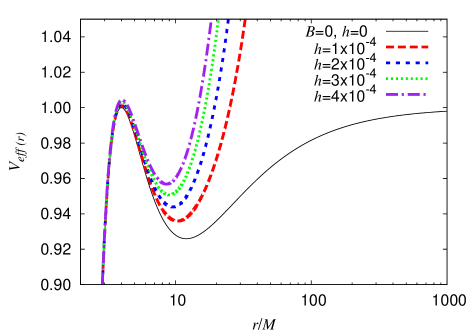
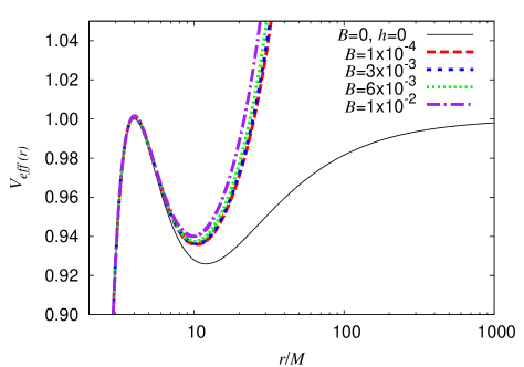
Figure 2: The effective potential for a perturbed Scwarzschild black hole of a total mass $M$ and specific angular momentum $\widetilde{L}=4M$. The solid line is the effective potential for a Schwarzschild black hole with the same total mass ($B=0$ and $K=0$). On the left plot $B$ is set to $10^{-4}M^{-1}$ and the parameter $h$ is running, while on the right $h=10^{-4}M^{-2}$ is fixed and different values of $B$ are taken.

In Fig 3 we present the radial dependence of the angular frequency, specific energy and specific angular momentum of the orbiting particle. All of these radial profiles indicate the perturbative presence of the asymptotically uniform magnetic field. Close to the black hole the rotational velocity $\Omega$ resembles the unperturbed Schwarzschild value. For higher radii, however, each radial profile of $\Omega$ has a less steep fall-off compared to the one for a standard accretion disk in the non-perturbed system. Moreover, at certain radii $\Omega$ is starting to increase. This unphysical model feature is explained in the following subsection. The radial profiles of $\widetilde{E}$ and $\widetilde{L}$ are also unbounded as $r\rightarrow\infty$.

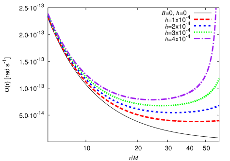
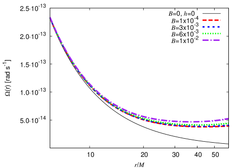
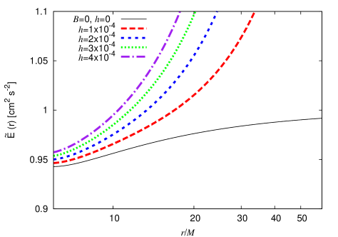
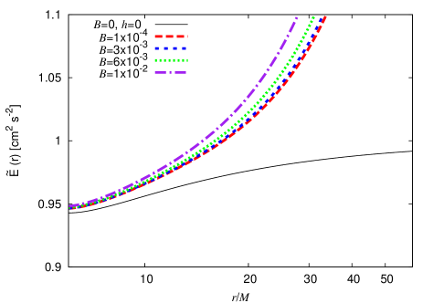
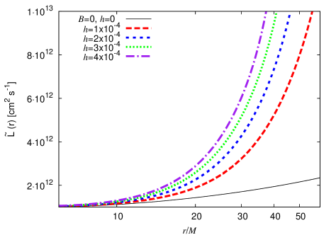
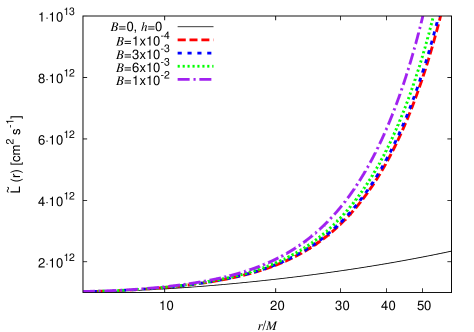
Figure 3: The angular velocity $\Omega$, specific energy $\widetilde{E}$ and specific angular momentum $\widetilde{L}$ of particles orbiting around a perturbed Schwarzschild black hole of total mass $M$. The solid line is the effective potential for a Schwarzschild black hole with the same total mass ($B=0$ and $K=0$). On the left plot $B$ is set to $10^{-4}M^{-1}$ and the parameter $h$ is running, while on the right $h=10^{-4}M^{-2}$ is fixed and different values of $B$ are taken.

IV.2 Photon flux and disk temperature

By inserting Eqs. (21)-(23) into Eq. (1) and evaluating the integral we obtain the flux over the entire disk surface. This enables us to derive the temperature profile and spectrum of the disk. As shown in Appendix B, the components $T_{t}^{r}$ $T_{t}^{z}$, $T_{\varphi}^{r}$ and $T_{\varphi}^{z}$ of the energy-momentum tensor for the magnetic field vanish. Since only these quantities appear in the integral form of the conservation laws of energy and angular momentum specified for the steady-state equatorial approximation, the magnetic field does not contribute to the photon flux radiated by the accretion disk at all. Therefore, for a Schwarzschild black hole with magnetic perturbation we can employ the same flux formula as for vacuum.

In Fig 4 we plot the flux integral (1) for a black hole with mass $2\times 10^{6}M_{\odot}$ and an accretion rate of $2.5\times 10^{-6}M_{\odot}$/yr, with the same sets of values for the parameters $B$ and $K$ as for the effective potential. An increase of the parameters $B$ and $K$ results in smaller radii of both the marginally stable and largest radius bound orbits, which shifts both the inner and outer edges of the accretion disc towards the black hole. This can be seen in the plots of the flux emitted by the disk where the radial flux profiles shift to lower radii, compared with the radial distribution of $F(r)$ for an accretion disk in Schwarzschild geometry.

A closer comparison of the flux profile shapes with $\Omega\left(r\right)$ on Fig 3 shows that for each parameter set the radius $r_{2}$ where $F\left(r\right)=0$ holds is precisely where $\Omega$ starts to increase. Going further outwards the flux would turn negative, indicating that the thin disk model breaks down at larger distances. Therefore we should consider our thin accretion disk only extending between $r_{ms}$ and $r_{2}$, letting the condition $F\left(r\right)=0$ to determine the outer radius of the thin disk.

On the graphs the approximate ranges of the perturbing parameters are $B\in\left(10^{-4},10^{-2}\right)M^{-1}$ and $K\in\left(10^{-4},4\times 10^{-4}\right)M^{-2}$. For these parameters $\eta_{B}\in\left(10^{-8},10^{-4}\right)\varepsilon^{-2}$ and $\eta_{K}\in\left(10^{-4},4\times 10^{-4}\right)\varepsilon^{-2}$, where $\varepsilon=M/\bar{r}$ is the post-Newtonian parameter. Thus the maximum values of both parameters $\eta_{B}$ and $\eta_{K}$ are of the order $10^{-4}\varepsilon^{-2}$. As the accretion can be discussed only in the range where both the magnetic field and tidal effects can be considered as perturbations of the Schwarzschild black hole, both parameters $\eta_{B}$ and $\eta_{K}$ have the upper limit $10^{-1}$. Therefore $10^{-4}\varepsilon^{-2}\lesssim 10^{-1}$ and $\varepsilon=M/r\gtrsim 10^{-3/2}$. As a consequence, the validity of the perturbed black hole picture holds in the range

$$2M\lesssim\bar{r}\lesssim 10^{3/2}M\approx 31M~{}.$$ (24)

The estimate of $r_{1}\approx 31M$ is in the range of the values for $r_{2}$ readable from Fig 4. We have seen earlier that the perturbed black hole picture can be extended up to $r_{1}$ only. Accretion disks are expected to exist only around central objects. In the regions where the space-time is closer to a uniform magnetic field perturbed by a black hole, rather than vice-versa, it is to be expected that accretion disks should not exist at all. As a first symptom of this, by increasing the radius the thin disk approximation should become increasingly inaccurate. This is the reason why the radius $r_{2}$, where the thin disk approximation breaks down, has to be connected with $r_{1}$.

We note that $r_{2}$ is more affected by the change of $B$ or $K$ then $r_{ms}$. For stronger perturbations the accretion disk is therefore located closer to the black hole and its surface area is reduced. However, the stronger magnetic field or higher value of $K$ increases the maximal intensity of the radiation without causing any significant shift in the peak of maximal flux.

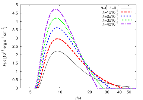
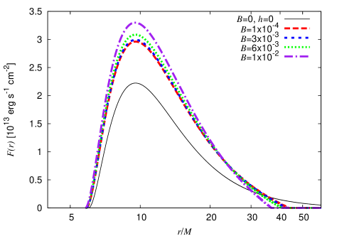
Figure 4: The time-averaged flux radiated by the accretion disk around a perturbed Schwarzschild black hole of total mass $M=2\times 10^{6}M_{\bigodot}$. The accretion rate is $2.5\times 10^{-6}M_{\bigodot}$/yr. The solid line is the radiated flux for a Schwarzschild black hole with the same total mass ($B=0$ and $K=0$). On the left plot $B$ is set to $10^{-4}M^{-1}$ and the parameter $h$ is running, while on the right $h=10^{-4}M^{-2}$ is fixed and different values of $B$ are taken.

Similar signatures can be recognized in the radial profiles of the disk temperature, shown in Fig 5 for the same parameter set of $B$ and $K$ (or $h$).

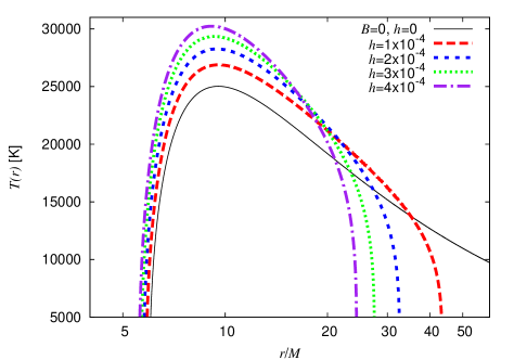
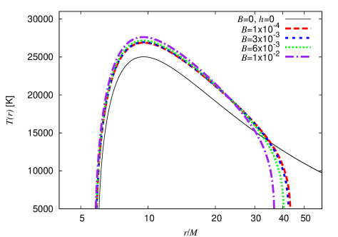
Figure 5: The temperature profiles of an accretion disk around a perturbed Schwarzschild black hole of total mass $M=2\times 10^{6}M_{\bigodot}$. The accretion rate is $2.5\times 10^{-6}M_{\bigodot}$/yr. The solid line is the temperature profile for a Schwarzschild black hole with the same total mass ($B=0$ and $K=0$). On the left plot $B$ is set to $10^{-4}M^{-1}$ and the parameter $h$ is running, while on the right $h=10^{-4}M^{-2}$ is fixed and different values of $B$ are taken.

IV.3 Disk spectrum

The spectrum of the disk is derived from Eq. (2) and represented with the same values of the perturbations as for the other plots. The characteristic shape of the spectra on Fig 6 shows a uniform increase at low frequencies (on a logarithmic scale) followed by a sharp decrease at high frequencies, ending in a cut-off at $\sim 10^{16}$ Hz. Moreover, we note that in the presence of perturbations the spectrum is blue-shifted in comparison with the Schwarzschild case. The shift of the spectrum towards higher energies indicates that besides the accreted mass-energy also some magnetic field energy is converted into radiation.

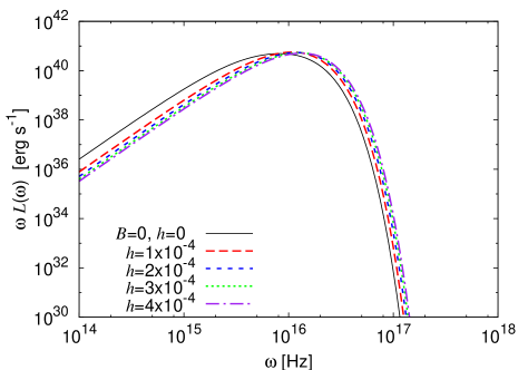
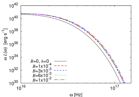
Figure 6: The disk spectra for a perturbed Schwarzschild black hole of total mass $M=2\times 10^{6}M_{\bigodot}$. The accretion rate is $2.5\times 10^{-6}M_{\bigodot}$/yr. The solid line is the disk spectrum for a Schwarzschild black hole with the same total mass ($B=0$ and $K=0$). On the left plot $B$ is set to $10^{-4}M^{-1}$ and the parameter $h$ is running, while on the right $h=10^{-4}M^{-2}$ is fixed and different values of $B$ are taken.

Finally, we give the conversion efficiency $\epsilon$ of the accreting mass into radiation in the perturbed system for the different values of the parameters $B$ and $K$ employed earlier in our analysis. In Table 1 we give both the marginally stable orbit, at which the specific energy is evaluated in the calculation of $\epsilon$ given in Eq. (3), and the efficiency for the indicated values of the parameters. As the perturbation parameters increase, both $r_{ms}$ and the efficiency of energy generation by accretion decrease.

$B[M^{-1}]$	$h[M^{-2}]$	$r_{ms}[M]$	$\epsilon$
0	0	6.00	0.0572
$10^{-4}$	$10^{-4}$	5.86	0.0537
	$2\times 10^{-4}$	5.75	0.0503
	$3\times 10^{-4}$	5.67	0.0469
	$4\times 10^{-4}$	5.59	0.0437
$2\times 10^{-3}$	$10^{-4}$	5.85	0.0532
$8\times 10^{-3}$		5.83	0.0526
$10^{-2}$		5.81	0.0520

Table 1: The marginally stable orbit and the conversion efficiency $\epsilon$ of the magnetically perturbed Schwarzschild black hole for different parameters $B$ and $K$ (or $h$).

V Concluding Remarks

Astronomical observations of the accretion disks rotating around black holes can provide both the spatial distribution (if the disk morphology is resolved) and the spectral energy distribution of the thermal radiation emitted by the disk. The radial flux profile and spectrum in the standard thin disk model can in turn be calculated for various types of compact central bodies with and without magnetosphere. Then a convenient way to determine the mass and the spin of the central black hole is to fit the flux profile and the spectrum derived from the simple disk model on the observational data. For static black holes, the analysis of the deviations of the disk radiation from the Schwarzschild case could indicate the presence of a magnetic field.

In this paper we have discussed the mass accretion process in the region of the Preston-Poisson space-time representing a Schwarzschild black hole perturbed by a weak magnetic field (which is however asymptotically uniform) and a distant tidal structure. For this we have (a) determined the region where this interpretation holds; (b) corrected the dynamical equations of test particles valid in the equatorial plane; and (c) applied the hydrodynamic approximation for the orbiting plasma.

The study of the perturbations included in the accretion process showed that (i) the thin disk model can be approximately applied until the radius where the perturbed Schwarzschild black hole interpretation holds; (ii) the accretion disk shrinks and the marginally stable orbit shifts towards the black hole with the perturbation; (iii) the intensity of the radiation from the accretion disk increases, while the radius where the radiation is maximal remains unchanged; (iv) the spectrum is slightly blue-shifted; and finally (v) the conversion efficiency of accreting mass into radiation is decreased by both the magnetic and the tidal perturbations.

We represent the system under discussion on Fig 7.

Figure 7: The black hole horizon, the thin accretion disk (between $r_{ms}=5.8M$ and $r_{1}=31M$) and the magnetic field topology (for $B=10^{-2}M^{-1}$).

Although the topology of magnetospheres around black holes is likely to be more complicated than the simple model considered here, the blue shifted disk spectrum indicating that some of the magnetic field energy also contributes to the radiation may be a generic feature, signaling the presence of a magnetic field. This conjecture is supported by the recent finding that symbiotic systems of black holes in fast rotation, accretion disk, jets and magnetic fields have a very similar magnetic field topology to the one represented on Fig 7, consisting of open field lines only KGB .

VI Acknowledgements

We thank Sergei Winitzki for interactions in the early stages of this work. LÁG is grateful to Tiberiu Harko for hospitality during his visit at the University of Hong Kong. LÁG was partially supported by COST Action MP0905 ”Black Holes in a Violent Universe”. MV was supported by OTKA grant no. NI68228.

Appendix A The curvature scalars on the horizon

In this Appendix we give the curvature scalars of the Preston-Poisson metric (5). Throughout the computations (except otherwise stated) the coordinates (9)-(10) of Konoplya are used. The results are valid up to $(B^{2},K)$ order. We found that:

(i) The perturbations are such that the Ricci scalar vanishes to $(B^{2},K)$ order, $R=0$.

(ii) With the use of light-cone gauge coordinates the Kretschmann scalar $\mathcal{K}=R_{abcd}R^{abcd}$ is

$$\mathcal{K}=\frac{48M}{r^{6}}\left[M+Kr^{3}\left(2-3\sin^{2}\theta\right)\right]~{},$$ (25)

which on the horizon (7) becomes

$$\mathcal{K}_{|r=r_{H}}=\frac{3}{4M^{4}}\left[1+16M^{2}K-4M^{2}(B^{2}+6K)\sin^{2}\theta\right]~{}.$$ (26)

Since the Ricci scalar vanishes the contraction of the Weyl tensor gives the same expression, $C_{abcd}C^{abcd}=\mathcal{K}$.

The Kretschmann scalar calculated in the Konoplya coordinates (9)-(10) is

$$\mathcal{K} = \frac{48M}{\bar{r}^{6}}\{M+2MB^{2}\bar{r}(2M-\bar{r})-2K\bar{r}(4M^{2}-2M\bar{r}-\bar{r}^{2})$$ (27)

$$+\bar{r}[3K(4M^{2}-2M\bar{r}-\bar{r}^{2})-2MB^{2}(3M-\bar{r})]\sin^{2}\theta\}\ ,$$

which agrees with (25) after the coordinate transformation (10).

(iii) The contraction of the Weyl tensor with the Killing vectors $t^{a}=(1,0,0,0)$ and $\phi^{a}=(0,0,0,1)$ is

$$C_{abcd}t^{a}\phi^{b}t^{c}\phi^{d}=C_{0303} = \frac{(2M-\bar{r})\sin^{2}\theta}{3\bar{r}^{2}}\{3M+[K(4M^{2}-4M\bar{r}+3\bar{r}^{2})-2MB^{2}(M-\bar{r})]\bar{r}$$ (28)

$$+3M[2K(M^{2}-M\bar{r}-\bar{r}^{2})-B^{2}(M^{2}-M\bar{r}+\bar{r}^{2})]\sin^{2}\theta\}~{}.$$

This quantity vanishes on the horizon. The contraction of the Killing vectors with the Riemann tensor gives the same result since $R_{0303}=C_{0303}$.

(iv) The second order scalar invariants of the Riemann tensor are

$$R_{\ abcd}^{\ast}R^{abcd} = {}^{\ast}R_{abcd}R^{abcd}=0\ ,$$

$${}^{\ast}R_{\ abcd}^{\ast}R^{abcd} = -\frac{16M}{\bar{r}^{10}\sin^{2}\theta}\{3M+2[2B^{2}M(7M-4\bar{r})-K(28M^{2}-16M\bar{r}-3\bar{r}^{2})]\bar{r}$$ (29)

$$-3[2B^{2}M(7M-3\bar{r})-K(28M^{2}-16M\bar{r}-3\bar{r}^{2})]\bar{r}\sin^{2}\theta\}\ ,$$

where $R_{\ abcd}^{\ast}=e_{cd}^{\ \ pq}R_{abpq}/2$, ${}^{\ast}R_{abcd}=e_{ab}^{\ \ pq}R_{pqcd}/2$ and ${}^{\ast}R_{\ abcd}^{\ast}=e_{ab}^{\ \ pq}e_{cd}^{\ \ rs}R_{pqrs}/4$, and $e_{abcd}$ is the antisymmetric Levi-Civita symbol. Similar contractions with the Weyl tensor give identical results.

On the horizon, the Euler scalar becomes

$${}^{\ast}R_{\ abcd}^{\ast}R^{abcd}=-\frac{1}{64M^{8}\sin^{2}\theta}\{3-4M^{2}[2(B^{2}-8K)+3(B^{2}+8K)\sin^{2}\theta]\}\ .$$ (30)

In conclusion, as the Kretschmann scalar $\mathcal{K}$ and the scalar ${}^{\ast}R_{\ abcd}^{\ast}R^{abcd}$ exhibit a $\theta$-dependence on the horizon, we conclude that despite the spherical shape of the horizon in the Konoplya coordinates, it has acquired a quadrupolar deformation due to the perturbing magnetic and tidal effects.

Appendix B The energy-momentum tensor

Since the coordinate transformation from the Eddington-Finkelstein type coordinates $(v,r,\theta,\varphi)$ to Konoplya coordinates Konoplya does not affect the angular variables $\theta$ and $\varphi$ the form of the vector potential (4) remains unchanged in the new coordinate system. Then the nonvanishing mixed components of the energy momentum tensor can be written in Konoplya coordinates as

$$T^{t}_{\ t} = \frac{B^{2}}{8\pi\bar{r}}(2M\sin^{2}\theta-\bar{r})\ ,$$

$$T^{\bar{r}}_{\ \bar{r}} = -\frac{B^{2}}{8\pi\bar{r}}(2M-\bar{r}-2(M-\bar{r})\cos^{2}\theta)\ ,$$

$$T^{\bar{r}}_{\ \theta} = -\frac{B^{2}}{4\pi}(2M-\bar{r})\cos\theta\sin\theta\ ,$$

$$T^{\theta}_{\ \bar{r}} = \frac{B^{2}}{4\pi\bar{r}}\cos\theta\sin\theta\ ,$$

$$T^{\theta}_{\ \theta} = \frac{B^{2}}{8\pi\bar{r}}(2M-\bar{r}-2(M-\bar{r})\cos^{2}\theta)\ ,$$

$$T^{\varphi}_{\ \varphi} = -\frac{B^{2}}{8\pi\bar{r}}(2M\sin^{2}\theta-\bar{r})\ .$$ (31)

Transforming these tensor components from the Konoplya coordinates to the coordinate system $x^{a^{\prime}}=(t,\bar{r},z=\bar{r}\cos\theta,\varphi)$ adapted to the equatorial plane, we obtain

$$T^{t}_{\ t}=T^{\ t}_{t} = \frac{B^{2}}{8\pi\bar{r}^{3}}[2M(\bar{r}^{2}-z^{2})-\bar{r}^{3}]\ ,$$

$$T^{\bar{r}}_{\ \bar{r}}=T^{\ \bar{r}}_{\bar{r}} = \frac{B^{2}}{8\pi\bar{r}^{3}}[\bar{r}^{3}-2M(\bar{r}^{2}+z^{2})]\ ,$$

$$T^{\bar{r}}_{\ z}=T^{\ \bar{r}}_{z} = \frac{B^{2}}{4\pi\bar{r}^{2}}(2M-\bar{r})z\ ,$$

$$T^{z}_{\ \bar{r}}=T^{\ z}_{\bar{r}} = -\frac{B^{2}}{2\pi\bar{r}^{2}}Mz\ ,$$

$$T^{z}_{\ z}=T^{\ z}_{z} = \frac{B^{2}}{8\pi\bar{r}^{3}}[2M(\bar{r}^{2}+z^{2})-\bar{r}^{3}]\ ,$$

$$T^{\varphi}_{\ \varphi}=T^{\ \varphi}_{\varphi} = \frac{B^{2}}{8\pi\bar{r}^{3}}[2M(z^{2}-\bar{r}^{2})+\bar{r}^{3}]\ .$$ (32)

Since the components $T^{r}_{t}$, $T^{z}_{t}$ $T^{r}_{\varphi}$ and $T^{z}_{\varphi}$ vanish identically, they do not appear in the expressions $E^{a}=-T^{a}_{\ b}t^{b}$ and $J^{a}=T^{a}_{\ b}{\varphi}^{b}$ of the energy and angular momentum flux 4-vectors and, in turn, do not give any contributions to the integrated laws of energy and angular momentum conservation.

References

- (1) N. I. Shakura and R. A. Sunyaev, Astron. Astrophys. 24, 33 (1973).
- (2) I. D. Novikov and K. S. Thorne, in Black Holes, ed. C. DeWitt and B. DeWitt, New York: Gordon and Breach (1973).
- (3) R. D. Blandford and R. L. Znajek, Month. Not. Roy. Astr. Soc. 179, 433 (1977).
- (4) L. X. Li, Astron. Astrophys. 392, 469 (2002).
- (5) D. X. Wang, K. Xiao, and W. H. Lei, Month. Not. Roy. Astr. Soc. 335, 655 (2002).
- (6) M. Camenzind, Astron. & Astroph. 156, 137, 1 62, 32 (1986).
- (7) M. Takahashi, S. Nitta, Y. Tamematsu, and A. Tomimatsu, Astrophys. J. 363, 206 (1990).
- (8) A. Janiuk, B. Czerny, Month. Not. Roy. Astr. Soc. In press (2011), E-print: arXiv:1102.3257.
- (9) Z. Kovács, L. Á. Gergely, and P. L. Biermann, Month. Not. Roy. Astr. Soc., in press (2011), E-print: arXiv:1007.4279.
- (10) D. A: Uzdensky, Astrophys. J. 603, 652 (2004).
- (11) B. Preston and E. Poisson, Phys. Rev. D 74, 064010 (2006).
- (12) K. Kuchař, Phys. Rev. D 50, 3961 (1994).
- (13) F. J. Ernst, J. Math. Phys. (N.Y.) 17, 54 (1976). W. A. Hiscock, J. Math. Phys. (N.Y.) 22, 1828 (1981). F. J. Ernst and W. J. Wild, J. Math. Phys. (N.Y.) 17, 182 (1976).
- (14) S. W. Hawking and J. B. Hartle, Commun. Math. Phys. 27, 283 (1972).
- (15) R. A. Konoplya, Phys. Rev. D 74, 124015 (2006).
- (16) R. M. Wald, Phys. Rev. D 10, 1680 (1974).
- (17) D. N. Page and K. S. Thorne, Astrophys. J. 191, 499 (1974).
- (18) K. S. Thorne, Astrophys. J. 191, 507 (1974).