Few emitters in a cavity: From cooperative emission to individualization

Abstract

We study the temporal correlations of the field emitted by an electromagnetic resonator coupled to a mesoscopic number of two-level emitters that are incoherently pumped by a weak external drive. We solve the master equation of the system for increasing number of emitters and as a function of the cavity quality factor, and we identify three main regimes characterized by well distinguished statistical properties of the emitted radiation. For small cavity decay rate, the emission events are uncorrelated and the number of photons in the emitted field becomes larger than one, resembling the build-up of a laser field inside the cavity. At intermediate decay rates (as compared to the emitter-cavity coupling) and for few emitters, the statistics of the emitted radiation is bunched and strikingly dependent on the parity of the number of emitters. The latter property is related to the cooperativity of the emitters mediated by their coupling to the cavity mode, and its connection with steady state subradiance is discussed. Finally, in the bad cavity regime the typical situation of emission from a collection of individual emitters is recovered. We also analyze how the cooperative behavior evolves as a function of pure dephasing, which allows to recover the case of a classical source made of an ensemble of independent emitters, similar to what is obtained for a very leaky cavity. State-of-art techniques of Q-switch of resonant cavities, allied with the recent capability to tune single emitters in and out of resonance, suggest this system as a versatile source of different quantum states of light.

I Introduction

The interaction of an ensemble of identical two-level emitters with the electromagnetic field has been the subject of intense theoretical and experimental studies since the pioneering work of Dicke [1]. Among the others, superradiance (or superfluorescence) is the most celebrated effect; it is manifested as a transient effect by the delayed emission of an intense burst of light, after the atomic population has been totally inverted [2]. In essence, superradiance is characterized by the emergence of collective coherence, which leads to a strongly enhanced emission rate as compared to the case of uncorrelated emitters. Such striking consequences of the quantum interference effect in radiation-matter coupled systems has been the subject of an intense experimental interest both for atomic [2, 3] and solid state [4] ensembles. Early studies on the statistical properties of the emitted light have evidenced the role of quantum fluctuations in the initial stages of the superradiant emission [5, 7, 6]. Whereas superradiance usually appears in the transient regime, recent theoretical studies have evidenced other signatures of collective behavior in the steady state regime, e.g. when the two-level emitters are continuously excited by incoherent light [8, 9, 10, 11]. In these references, cooperative emission is obtained by coupling the emitters to a low quality ($Q$) cavity mode, which behaves as a collective channel of losses. As a matter of fact, strong confinement enhances the interaction of each emitter with the cavity field, eventually making it predominant with respect to individual relaxation channels. Collective dynamics can be induced this way, provided the atoms identically interact with the cavity mode, a condition much less stringent than in free space. Tuning the pumping power allows one to explore different regimes, leading to different intensities and statistics for the emitted radiation [10, 11]. In particular, it has been shown that when the pumping strength is too low to saturate a single emitter of the ensemble, the collection of two-level systems emits a highly bunched field [9, 11]. The strong temporal correlation has been attributed to the relaxation of the system in the subradiant states of the ensemble of emitters. These states behave as sources of photon pairs triggered by the driving pulses, hence the bunching effect in the correlation properties.

In this paper, we analyze the subradiant regime and go beyond previous works by keeping the cavity mode as a relevant degree of freedom. This situation is new with respect to previous theoretical studies, where the radiation mode was commonly eliminated by an adiabatic approximation. We show that the bunching degree decays with the number of emitters and oscillates with its parity, being larger when the number of emitters is even, upon converging to a single value as the number of emitters grows. We give an interpretation of this effect, based on the structure of Hilbert space of the system. Furthermore, keeping the cavity mode in the description allows to explore two other limits, depending on the cavity finesse. If this parameter is significantly increased, the strong coupling conditions lead to the emission of a field showing no temporal correlations, an effect that we identify with the emission of Poissonian radiation similar to a lasing transition. Recently, such regime has been investigated from the spectral point of view [12, 13], while here we address its statistical properties. On the contrary, for decreasing cavity finesse one progressively decreases the coupling with the mode, allowing to continuously explore the boundary between collective and individual behavior of such radiation sources. When all the emitters become uncorrelated, increasing their number one by one up to large values coincides essentially with building a classical source with chaotic statistical properties. Dipole correlation can also be destroyed with pure dephasing, a situation that we eventually explore as well.

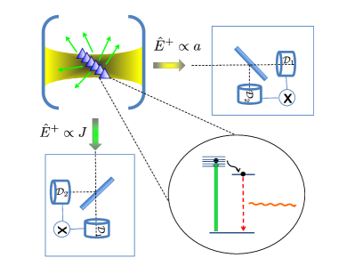
Figure 1: Schematic of the system under consideration in this work: $N$ two-level emitters incoherently pumped by an external drive, coupled to a single resonator mode. Correlations in the emitted field can be detected through a HBT set-up either from the cavity or from the emitters’ loss channel, respectively. A typical incoherent pumping scheme is shown, in which high-energy excitations relax down to a well defined ground state transition (e.g. through phonon scattering) via photon emission.

The present work becomes particularly relevant when considering that the subradiant regime is reachable if and only if each single emitter of the ensemble is predominantly coupled to the cavity mode. In particular, this allows to pump each emitter very slowly, but still faster than any individual relaxation mechanism. This is nowadays possible thanks to impressive progress in nano-fabrication technology on single emitter-cavity coupling [14, 15, 18, 16, 17, 19, 20, 24, 21, 22, 23, 25, 26, 27]. Small assemblies of artificial quantum emitters, like quantum dots [14] and superconducting qubits [15] coupled to a high-Q resonator mode have recently become available, strongly motivating to investigate the new physics provided by these systems. Moreover, beyond introducing an external parameter to control the steady state collective regime, this model is of great interest also for the study of lasing transition, as well as to investigate the connections between superradiance and lasing [28].

The paper is organized as follows. We first introduce the model and the methods employed to solve it, both numerically and analytically (Sec. II). Then, we present results as a function of cavity finesse, and we give a physical interpretation for the different regimes found (Secs. III, IV, and V). Before summarizing the main conclusions, we give a brief description of possible realistic implementations to explore the physics investigated in this work (Sec. VI).

II Model and methods

The system under study consists of $N$ two-level emitters coupled to the mode of an electromagnetic cavity of annihilation (creation) operator $a$ ($a^{\dagger}$) with equal coupling strength, $g$, and it is schematically pictured in Fig. 1. To focus on collective effects, we will assume that the resonator and all the emitters have the same transition frequency, $\omega$. The range of validity of this ideal model in practical implementations is discussed in Sec. VI. The model can be rigorously described by the Tavis-Cummings Hamiltonian (in the rotating wave approximation)

$$H=\sum_{i=1}^{N}\hbar\omega(\sigma_{z}^{i})+\hbar\omega a^{\dagger}a+ig(aJ_{+}-J_{-}a^{\dagger})\,,$$ (1)

where $J_{+}=\sum_{i}\sigma_{+}^{i}$ is the collective dipole operator, and $\sigma_{-}^{i}=|g_{i}\rangle\langle e_{i}|$ is the lowering operator of the single emitter $i$, whose excited (ground) state is denoted by $|e_{i}\rangle$ ($|g_{i}\rangle$). The Hilbert space corresponding to the assembly of resonant atoms is equivalent to the tensor product of the 2-dimensional space of each single emitter, i.e. $\mathcal{H}\simeq(\mathbb{C}^{2})^{\otimes N}$, spanned by the basis of factorized states in the form $|i_{1}\rangle|i_{2}\rangle...|i_{n}\rangle$, where $i_{n}=\{g_{n},e_{n}\}$ (in the following we shall refer to this basis as the uncoupled basis). When including possible dissipation channels and external driving, the Markovian dynamics of the full system is given by

$$\dot{\rho}=-i[H,\rho]+\sum_{i=1}^{N}\mathcal{L}_{i}(\rho)+\mathcal{L}_{a}(\rho)+\mathcal{L}_{\gamma^{*}}(\rho)\,.$$ (2)

The Lindblad dissipative terms, modeling incoherent loss and pumping of each emitter, explicitly read

$$\mathcal{L}_{i}(\rho) = \mathcal{L}_{\gamma}(\rho)+\mathcal{L}_{P_{x}}(\rho)$$ (3)

$$= \frac{\gamma}{2}(2\sigma_{-}^{i}\rho\sigma_{+}^{i}-\sigma_{+}^{i}\sigma_{-}^{i}\rho-\rho\sigma_{+}^{i}\sigma_{-}^{i})+$$

$$\frac{P_{x}}{2}(2\sigma_{+}^{i}\rho\sigma_{-}^{i}-\sigma_{-}^{i}\sigma_{+}^{i}\rho-\rho\sigma_{-}^{i}\sigma_{+}^{i})\,,$$

where the quantity $\gamma$ is the individual emission rate in loss channels distinct from the cavity mode for each emitter, and $P_{x}$ quantifies the excitation rate. As pictured in Fig. 1, incoherent pumping can be obtained by resonantly exciting higher energy states, that further relax down to the levels of interest. The decay of the cavity mode with rate $\kappa$ through imperfect mirrors is described by the following term

$$\mathcal{L}_{a}(\rho)=\frac{\kappa}{2}(2a\rho a^{\dagger}-a^{\dagger}a\rho-\rho a^{\dagger}a)\,$$ (4)

whereas the pure dephasing of the emitters, which is unavoidable in solid-state artificial atoms, can be taken into account by a Liouvillian term of the form [29]

$$\mathcal{L}_{\gamma^{*}}(\rho)=\sum_{i=1}^{N}\frac{\gamma^{\ast}}{2}(\sigma_{z}^{i}\rho\sigma_{z}^{i}-\rho)\,.$$ (5)

Following standard input-output theory [30], the output field at the photodetectors is proportional to the $a$ operator (and its conjugate). We are interested in the temporal correlations of the field radiated by the cavity mode. Experimentally, an ordinary Hanbury-Brown Twiss (HBT) setup can be used, giving access to the steady state second-order correlation at zero-time delay [31]

$$g_{a}^{(2)}(0)=g_{ss}^{(2)}=\langle a^{\dagger}a^{\dagger}aa\rangle/\langle a^{\dagger}a\rangle^{2}\,.$$ (6)

In order to calculate the latter quantity, we numerically solve Eq. (2) either by direct integration or by Quantum Monte Carlo (QMC) simulations [32, 33]. Direct integration allows one to obtain accurate results at lower computational time costs, for which we use an extension of the code already employed in a previous work [34]. However, the tensor structure of the phase space makes the computational resources needed for a direct integration rapidly diverge. On the contrary (wave function) QMC gives the solution as a stochastic average over quantum trajectories of wavefunctions unravelings, drastically reducing the amount of space needed and allowing us to push forward the previous computational limits [33].

If $\kappa$ is large enough, the cavity mode can be adiabatically eliminated from the equations, giving rise to an effective dynamics described by the reduced master equation

$$\dot{\rho}=\mathcal{L}_{\Gamma}(\rho)+\sum_{i=1}^{N}\mathcal{L}_{i}(\rho)\,,$$ (7)

where

$$\mathcal{L}_{\Gamma}(\rho)=\frac{\Gamma}{2}(2J_{-}\rho J_{+}-J_{+}J_{-}\rho-\rho J_{+}J_{-})\,.$$ (8)

The physical meaning of this equation is the following: the cavity acts as a common relaxation channel for the atoms, whose dissipation rate is quantified by the coupling strength with the collective atomic dipole $J_{-}$, i.e. $\Gamma=4g^{2}/\kappa$. Namely, adiabatic elimination is valid when $\kappa\gg N\Gamma$ [10]. In this regime, the cavity field, and thus the output field is proportional to the collective dipole degree of freedom, $J_{-}$. Consequently, the temporal autocorrelation function at zero time delay can be expressed as

$$g_{J}^{(2)}(0)=\langle J_{+}J_{+}J_{-}J_{-}\rangle/\langle J_{+}J_{-}\rangle^{2}\,.$$ (9)

Note that the same detection properties could be obtained by registering the far field where the atomic dipoles interfere, as it is pictured in Fig. 1. Also for Eq. (9) we can employ numerical approaches either based on direct integration or on QMC, respectively. As usual, once the master equation is solved for $\rho$ the expectation values can be calculated with the general rule $\langle\hat{O}\rangle=\mathrm{Tr}\{\hat{O}\rho\}$, where $\hat{O}$ identifies the operator corresponding to a given observable.

Sweeping the cavity finesse allows to continuously explore the transition from a collective behavior driven by $\mathcal{L}_{\Gamma}(\rho)$ to an individual one, corresponding to $\mathcal{L}_{i}(\rho)$. In this work we analytically study some limits of these regimes. If the dynamics is individual, it is naturally described in the uncoupled basis mentioned above. If the dynamics is collective, an order appears in the system due to the build up of correlations between dipoles belonging to different atoms [2], manifested by the occurrence of coherences in the uncoupled basis. In the latter case, a natural basis is provided by the eigenstates $|J,M\rangle$ of the total angular momentum $\{J^{2},J_{z}\}$ (in the following, we shall talk about the coupled basis of the atomic states). Note that among them, the states satisfying $J_{-}|J,M\rangle=0$ are not coupled to the electromagnetic field and are thus defined as “subradiant”.

III Second-order correlations of the emitted field

As mentioned above, the regime studied in the literature so far is the adiabatic elimination regime, where the cavity mode operator can be assumed as $a\propto J_{-}$. We assume a fixed and weak incoherent pumping rate, $P_{x}/g$. In order to understand the collective behavior and to link it to the previous literature, we plot in Fig. 2a the average cavity mode occupation, $n_{a}=\langle a^{\dagger}a\rangle$, the average collective occupation of the emitters, $n_{J}=\langle J_{+}J_{-}\rangle$, and the total emitters population, $Nn_{x}$ (where $n_{x}=\langle\sigma_{+}^{i}\sigma_{-}^{i}\rangle$ in the steady state. The second-order correlations are plotted in Fig. 2b, and they have been calculated both from the cavity mode operator, Eq. (6), and the collective dipole operator, Eq. (9), respectively. The results are shown for $N=5$ emitters in the cavity, which represents a good compromise to simultaneously have a well converged numerical solution for Eq. (6) and to evidence the effects of collective behavior. As it can be seen in Fig.  2b, the two calculated correlations don’t match for most of the parameter space, showing that the cavity mode has to be taken into account to obtain the correct result when the cavity finesse is large. The two curves converge to the same value when $\kappa/g\simeq 50$, where the adiabatic approximation starts to be satisfied.

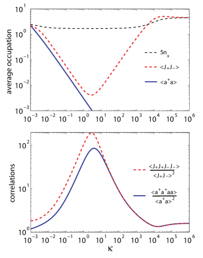
Figure 2: Full numerical results for average populations and second-order correlation in steady state as a function of $\kappa$ (normalized to $g$) for the case of $N=5$ atoms in the cavity, calculated from atomic and cavity fields, respectively. Parameters are: $P_{x}=0.001g$, $\gamma=0.0001g$.

We first focus on the case where adiabatic elimination is valid: two different situations emerge. The case where $\Gamma=4g^{2}/\kappa>\gamma$ corresponds to a collective dynamical behavior for the atomic ensemble. In the low pumping regime under study, the emitted field is strongly bunched, $g^{(2)}(0)>1$, confirming previous theoretical works [9, 11] on a similar model. In the two-atom case, this behavior has been attributed to the emission of so called “super-radiant” photon pairs [9], typically separated by a delay scaling like the inverse of the pumping rate. This regime has been further explored for a larger number of emitters in [10, 11], where the authors show that the atomic ensemble has mostly relaxed in the subradiant states. This is in agreement with Fig. 2a where the average intensity emitted by uncorrelated atoms, $Nn_{x}$ is compared to the average fluorescence field emitted by the collective atomic dipole, $\langle J_{+}J_{-}\rangle$. It can be clearly observed that in a $\kappa/g$ range spanning several decades, the condition $\langle J_{+}J_{-}\rangle<Nn_{x}$ is usually satisfied, a signature of the anticorrelation of the atomic dipoles and of the efficient relaxation in the sub-radiant states. Note that the subradiant regime is reached when $P_{x}<\Gamma$, a condition that is not fulfilled anymore for $\kappa/g>10^{3}$. In that case the steady state emission becomes super-radiant, i.e. $\langle J_{+}J_{-}\rangle>Nn_{x}$, and correspondingly $g^{(2)}(0)$ approaches $1$, a limit that is exactly reached only for $N\gg 1$ as evidenced in previous work [11]. Finally, when $\kappa/g$ is increased up to a point where $\gamma>\Gamma$ (very bad cavity regime), emission appears as if it was coming from an independent collection of emitters. Under such conditions, the limiting values are such that $\langle J_{+}J_{-}\rangle\to Nn_{x}$ and $g^{(2)}(0)\to 2(1-1/N)$, a limit that we analyze in detail below.

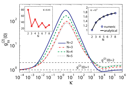
Figure 3: Full numerical solution for zero time delay second-order correlation in steady state calculated from the cavity degree of freedom, as a function of $\kappa$ (normalized to $g$), for low incoherent pump rate $P_{x}=0.001g$ and emitters’ dissipation $\gamma=0.0001g$, and varying number of emitters, $N$. Left inset: oscillations as a function of $N$ in the good cavity, subradiant regime. Right inset: bad cavity limit of correlations as a function of $N$.

We focus now on the statistical properties of the system by looking at the dependence on the number of emitters, the results are shown in Fig. 3 with the same parameters used in Fig. 2. Keeping the cavity mode as a relevant degree of freedom allows one to explore the temporal correlations on the entire $\kappa/g$ range, which can only be done by the full numerical solution of the master equation. At this point, we go beyond previous works. First, we notice that a transition to amplified spontaneous emission clearly occurs for very large cavity finesse, i.e. as soon as $\kappa/g<0.001$ ($P_{x}>\kappa$), with the temporal fluctuations becoming Poissonian independently of the number of emitters. A temporal picture for this effect is that as soon as $P_{x}>\kappa$, the cavity stores the photons on a timescale longer that the typical delay between two emission events by the atomic assembly, blurring out any temporal correlation feature. This situation has been already evidenced for the single emitter case in [34, 35, 36], and it was identified as a lasing threshold signature. Here, the system becomes a source of radiation with Poissonian statistical noise, reminiscent of a few emitters laser. The case for $N=2$ in the strong emitter-cavity coupling regime was also studied for a similar model in Ref. [37, 38] as a function of pump power. As a matter of fact, three main effects on measurable quantities can be identified: (i) the average cavity population becomes larger than one, setting the onset of stimulated emission (see also Fig. 2a), (ii) the population of each emitter is clamped to a definite value, here, $n_{x}\simeq 0.5$ (i.e. $5n_{x}\to 2.5$ in Fig. 2a), and (iii) $g^{(2)}(0)\to 1$ (more clearly evidenced in Fig. 3 for any $N=2,3,4,5$).

On increasing $\kappa/g$, it is evident from Fig. 3 that in the subradiant range there is an unexpected and quite pronounced parity-dependent oscillation of the photon correlation value at zero-time delay, a behavior that has not been discussed in the literature, to our knowledge. Such parity oscillations are not limited to the adiabatic elimination region (see the inset on the left panel for $\kappa/g=0.45$ and up to a number of emitters $N=8$). The latter calculation required consistent numerical optimization and was performed on a cluster, where the full master Eq. (2) could be solved without truncation effects on the convergence. Although quite difficult to be analyzed in the dressed state picture, the oscillatory behavior of correlations as a function of the number of emitters can be roughly interpreted as a consequence of the collective coupling in Eq. (8), which dominates the dynamics over the individual relaxation channels in Eqs. (3) and (4). The former couples the states with the same quantum number $J$ and is diagonal in the coupled basis. On the contrary, the other channels act on each emitter and are responsible for coherences between states with different values of $J$. We will investigate this regime in detail in Sec. IV. The bunching behavior reaches a maximum for $\kappa\simeq g$, slightly depending on the number of emitters. An interesting even/odd behavior has also been found in the spectral response [12] and it would be interesting to relate the two phenomena in future developments of the present work.

Finally, in the opposite limit of $\kappa/g$ becoming large enough that $\gamma>\Gamma$ the radiation is characterized by a field emitted from independent atoms. Oscillations tend to disappear, as it can be seen in Fig. 3 (see also inset on the right hand side). In this regime, the single emitters undergo individual dynamics, and the dipoles become uncorrelated (see also the large $\kappa$ limit in Fig. 2a, where $\langle J_{+}J_{-}\rangle\to Nn_{x}$. Restricting our considerations to the correlation function, an analytical expression of $g^{2}(0)$ is derived in Sec. V, where we show that $g^{(2)}(0)=2(1-1/N)$. Note that in the limit of a large number of atoms, $g^{(2)}(0)\to 2$, which corresponds to the emission of an incoherent chaotic field.

IV Parity-related oscillations

In this Section we calculate analytical expressions for the bunching degree of the emitted field, in the two and three emitters cases, which provide a physical explanation for the observed parity dependence. The analytic treatment is valid in the regime of adiabatic elimination of the cavity mode dynamics. To sustain our analysis, we have also used a Quantum Monte Carlo (QMC) simulation [33]. We have calculated $g^{(2)}(0)$ as a function of the number of emitters $N$, with $N$ being as large as $10$. The results are plotted in Fig. 4a by simulating the reduced master equation, Eq. (7). As it can be seen, we alternatively recovered the result shown in Fig. 3 at a specific value of $\kappa/g=100$, by generalizing to a larger number of emitters that would be unaccessible through direct numerical integration. Again, bunching and oscillatory behaviors are clear signatures of this collective low pumping regime, which we are going to analytically describe below.

IV.1 Two emitters case

In the following of this Section we use the coupled basis for the emitters. Such basis of states is schematically indicated in Fig. 4b. In particular, the two-emitter case is pictured in the first panel of Fig. 4b, and we will focus on this diagram here. In this specific case, the basis $|J,M\rangle$ is non-degenerate and the Hilbert space consists of the three symmetric (or Dicke) states $|1,1\rangle=|e_{1},e_{2}\rangle$, $|1,0\rangle=(|e_{1},g_{2}\rangle+|g_{1},e_{2}\rangle)/\sqrt{2}$, $|1,-1\rangle=|g_{1},g_{2}\rangle$, and the antisymmetric state $|0,0\rangle=(|e_{1},g_{2}\rangle-|g_{1},e_{2}\rangle)/\sqrt{2}$ (i.e., the usual triplet and singlet states of a spin 1 system). The steady state (and $g^{(2)}(0)$ statistics) is the result of a competition between collective (specifically $\mathcal{L}_{\Gamma}$) and individual decoherence channels (i.e., $\mathcal{L}_{P_{x}},\mathcal{L}_{\gamma},\mathcal{L}_{\gamma^{*}}$). The results shown in Fig. 4a are obtained without pure dephasing and with $P_{x}=10\gamma$. In the steady state, low pumping equally populates the subradiant states $|1,-1\rangle$ and $|0,0\rangle$. As it was first discussed by Temnov and Woggon [9], one can decompose the problem in two mutually exclusive cycles. In the regime under study, the $\Gamma$-related de-excitation events are much more probable than the excitation events driven by the pumping rate $P_{x}$. Hence, as soon as an excitation is stored in a state where the two mechanisms are possible, it is more likely that the excitation will undergo a collective emission than an upward pump jump. The microscopic scenario will then involve one cycle (pictured in green) consisting of the excitation and relaxation of the symmetric state $|1,0\rangle$, leading to the emission of single photons. In the other cycle (pictured in red), the excitation is first stored in $|0,0\rangle$. Then, during the time evolution, the only possibility is to excite the state $|1,1\rangle$, leading to the fast emission of two photons. The system prepared in the subradiant state $|0,0\rangle$ behaves thus like a deterministic source of photon pairs. Each pair is emitted on a timescale $1/\Gamma$, the delay between two pairs being typically $1/P_{x}$. Consequently, the emitted field is expected to show bunching, $g^{(2)}(0)\sim\Gamma/P_{x}$, an order of magnitude that we exactly recover below by analytically solving the approximate master equation.

In fact, to go beyond this qualitative interpretation we have computed the expression for $g^{(2)}(0)$ in terms of the relevant elements in the steady state density matrix

$$g^{(2)}(0)=\frac{\rho_{1,1}}{[\rho_{1,1}+\rho_{1,0}]^{2}}\,,$$ (10)

at first order in $P_{x}/\Gamma$. The diagonal matrix elements of the density matrix are written with the row (column) index only, e.g. $\langle J,M|\rho|J,M\rangle=\rho_{J,M}$. In this two-emitter case the evolution equations for the diagonal elements do not involve off-diagonal terms and the solution is obtained by solving a system of rate equations governing the evolution of the atomic populations. With lengthy but straightforward calculations, we express Eq. (7) on the basis above, and solve it for the steady state $\dot{\rho}=0$. We finally obtain an analytical estimation

$$g^{(2)}(0)=\frac{16}{9}\frac{g^{2}}{\kappa P_{x}}=\frac{4}{9}\frac{\Gamma}{\kappa P_{x}}\,,$$ (11)

which for $P_{x}/g=10^{-3}$ and $\kappa/g=100$ gives $g^{(2)}(0)\simeq 17.8$, a value that is very close to the numerical results (obtained from both direct numerical integration and QMC).

IV.2 Three emitters case

In the $N=3$ case, the simple picture above cannot be applied directly. The most important difference emerges immediately from the very nature of the Hilbert space. As pictured in Fig. 4b, right panel above, the $J=J_{\text{min}}=1/2$ subspaces have a 2-level system structure. As a consequence, the subradiant states corresponding to $|J_{min},-M_{J_{min}}\rangle$ do not behave as deterministic sources of photon pairs as in the $N=2$ case, but eventually give rise to single-photon cycles when they are pumped (light blue arrows in Fig. 4b). The presence of these extra loops spoils the bunching of the emitted field, and this gives a simple explanation for the abrupt loss of $g^{(2)}(0)$ bunching when going from two to three emitters.

To sustain this argument we have computed the second-order correlation $g^{(2)}(0)$ in terms of the density matrix elements, which for the $N=3$ case reads

$$g^{(2)}(0)=\frac{12(\rho_{\frac{3}{2},\frac{3}{2}}+\rho_{\frac{3}{2},\frac{1}{2}})}{[3\rho_{\frac{3}{2},\frac{3}{2}}+4\rho_{\frac{3}{2},\frac{1}{2}}+3\rho_{\frac{3}{2},-\frac{1}{2}}+\rho_{\frac{1}{2},\frac{1}{2};1}+\rho_{\frac{1}{2},\frac{1}{2};2}]^{2}}\,.$$ (12)

We followed the same notation as in Eq. (10) for the matrix elements. The subradiant states are written $|1/2,-1/2;1\rangle$ and $|1/2,-1/2;2\rangle$ [39], where the second label is a shorthand notation related to the $g=2$ extra degeneracy (see App. A and the related figure). After writing the master equation in this basis, we then proceeded with a perturbative solution of the linear system for the steady-state matrix elements in powers of $(P_{x}/\Gamma)$. Differently from the $N=2$ case, the equations of motion for the diagonal terms now involve off-diagonal matrix elements, preventing one from describing the dynamics with a simple set of rate equations. Nevertheless, within the same perturbative picture, we can consider these terms to be much smaller than the diagonal ones. Indeed, the coherences are brought by some residual individualization of the $P_{x}$-driven channel that, for the parameters chosen, acts as a perturbation over the collective dynamics induced by the $\Gamma$ events. The latter argument has been checked with the steady-state density matrix elements obtained numerically. As detailed in App. B, the final result reads

$$g^{(2)}(0)\simeq \frac{14}{75}\frac{\Gamma}{P_{x}}+2.067-3.501\frac{P_{x}}{\Gamma}+9.18\left(\frac{P_{x}}{\Gamma}\right)^{2}$$ (13)

$$-23.4\left(\frac{P_{x}}{\Gamma}\right)^{3}+\mathcal{O}\left(\frac{P_{x}}{\Gamma}\right)^{4}\,.$$

We obtain the analytical value $g^{(2)}(0)\simeq 9.46$, which compares very well with the numerically calculated value $\simeq 9.55$ reported in Fig. 4a from QMC simulations. Notice that the population of the state $|\frac{3}{2},\frac{3}{2}\rangle$ cannot be neglected and was also taken into account in the analytical calculation.

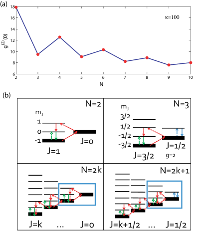
Figure 4: (a) Oscillations in the second-order correlation at zero time delay in the bad cavity, sub-radiant regime ($\kappa/g=100$). (b) Schematic energy level diagram for $N=2$ and $N=3$ in the total angular momentum basis, and their generalizations for even and odd number of emitters, respectively. For $N=3$, $g=2$ reminds the two-fold permutation degeneracy

IV.3 Generalization to $N>3$ emitters

Considering the energy level diagrams in the generic even and odd cases, as depicted in Fig. 4b, lower panels, one can always find the two patterns above (i.e., $N=2$ and $N=3$) as distinctive features of each scenario. For increasing number of emitters more subradiant states become available, among which the population arising from the $P_{x}$ reservoir will be shared (bold levels in the figure). This spreading of population unavoidably leads to the decay of the bunching degree as $N$ is increased, as observed in Figs. 3 and 4a, and confirmed by the general trend anticipated in [9] where a semi-classical approach was used. In the limit of large large numbers, such as $N=10000$, the bunching degree of $g^{(2)}(0)$ converged to $2$, as for classical chaotic sources. Note that in our case taking the limit of large numbers requires some caution, as one could exit the validity of the adiabatic elimination approximation, $\kappa\gg N\Gamma$, and eventually enter strong collective light-matter coupling regime (see, e.g., recent works [41, 42]). For the parameters chosen in the simulation in Fig. 4a, the condition for adiabatic elimination limits the maximum number of emitters to about 2000.

V Individualization

We consider now the case where the cavity finesse is decreased down to a point where the coupling of each emitter to the mode, $\Gamma$, becomes of the same order of magnitude of the coupling to its individual decay channel, $\gamma$. As we have seen in Figs. 2b and  3, this leads to totally uncorrelated emission events from the atomic dipoles. In this regime, which we define as the “individualization,” the parity-induced oscillations vanish and the bunching degree converges to $g^{(2)}(0)=2(1-1/N)$ (see Fig. 3, inset on the right), a behavior that we demonstrate below. Note that the same value for the parameter $g^{(2)}(0)$ has been computed in the strong pumping case [11]. As a matter of fact, a large pump power leads to total population inversion, a state where the dipoles necessarily become uncorrelated. Moreover, it is interesting to show in the context of the present work that an alternative way of obtaining a source of uncorrelated dipoles is to increase the pure dephasing rate, $\gamma^{*}$. The latter effect is shown in Fig. 5, where a full numerical solution based on direct integration has been employed for $\kappa/g=100$. It is evident that individualization is reached as soon as $\gamma^{*}>\Gamma$, washing out the oscillations and leading to the same limit for the second order correlation parameter, as clearly displayed in the inset.

For the sake of completeness, we have computed the steady state second-order correlation $g^{(2)}(\tau)$, for any delay $\tau$. Adiabatic elimination is valid and this quantity can be calculated as a function of the atomic operator, namely $g^{(2)}(\tau)={\langle J_{+}(0)J_{+}(\tau)J_{-}(\tau)J_{-}(0)\rangle}/{\langle J_{+}(0)J_{-}(0)\rangle^{2}}$. We make the assumption that the steady state of the ensemble can be factorized in the uncoupled basis, which is reasonable as each emitter behaves individually. Thus, developing (see App. C) the expression of $J_{\pm}$ with respect to the individual atomic operator $\sigma_{\pm}^{i}$ leads to

$$g^{(2)}(\tau)=\frac{\sum_{i}g_{i}^{(2)}(\tau)I_{i}^{2}+\sum_{i\neq k}I_{i}I_{k}\{1+g_{i}^{(1)}(\tau)^{*}g_{i}^{(1)}(\tau)\}}{(\sum_{i}I_{i})^{2}}\,,$$ (14)

where we have introduced the intensity per emitter, the first and the second order correlation functions for the quantum emitter $i$, as $I_{i}=\langle\sigma_{+}^{i}(0)\sigma_{-}^{i}(0)\rangle$, $g_{i}^{(1)}(\tau)=\langle\sigma_{+}^{i}(\tau)\sigma_{-}^{i}(0)\rangle/I_{i}$, $g_{i}^{(2)}(\tau)=\langle\sigma_{+}^{i}(0)\sigma_{+}^{i}(\tau)\sigma_{-}^{i}(\tau)\sigma_{-}^{i}(0)\rangle/I^{2}_{i}$, respectively. As initially mentioned in seminal lectures [43] and papers [44], and as it clearly appears in Eq. (14), the second order correlation function involves the emission of pairs of atomic excitations. When $\tau=0$, this expression simplifies to

$$g^{(2)}(0)=2(1-1/N)\,,$$ (15)

confirming our numerical simulations (see right inset of Fig. 2). The bunching at small delays is due to an interference resulting from the indistinguishability of the atoms in the emitting pairs [43]. Note that surprisingly, this behavior was never observed experimentally. As a matter of fact, the interference is washed out as soon as individual first order coherence, $g_{i}^{(1)}(\tau)$, vanishes [45, 46, 31, 47, 44]. This phenomenon takes place on the timescale of dephasing processes, leading to the following expression:

$$g^{(2)}(0)\simeq 1-1/N$$ (16)

eventually corresponding to a particle-like behavior. In fact, let’s consider $N$ independent sources each emitting classical identical particles one-by-one. Such a model-source is characterized by a total emission intensity $I=\sum_{i}I_{i}$ with $\langle I_{i}(t)I_{j}(t+\tau)\rangle=0$ if $i\neq j$. In the stationary regime we have $\langle I_{i}(t)\rangle=\langle I_{i}(t+\tau)\rangle=I_{0}$, since we suppose that the $N$ sources are characterized by the same main current. The total second order correlation signal is therefore

$$g_{\textrm{tot}}^{(2)}(\tau)=\frac{\langle I(t)I(t+\tau)\rangle}{\langle I(t)\rangle\langle I(t+\tau)\rangle}$$ (17)

which becomes

$$g_{\textrm{tot}}^{(2)}(\tau)=\frac{\sum_{i}g_{i}^{(2)}(\tau)+N(N-1)}{N^{2}}.$$ (18)

However, our $N$ idealized sources are single particle emitters i.e. $g_{i}^{(2)}(0)=0$. This clearly mimics the quantum-like behavior of two-level systems. Therefore, we get Eq. (16). Interestingly, from basic textbook quantum optics we obtain for a pure $|n\rangle$ photon Fock state the expression $g^{(2)}(0)=1-{1}/{n}$. The result is therefore also intuitive from this point of view.

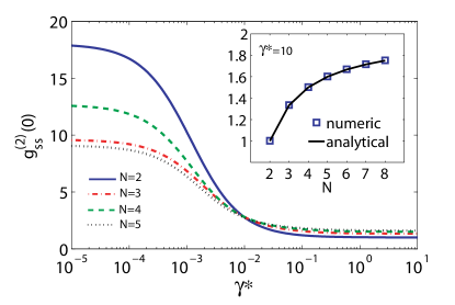
Figure 5: Zero time delay second-order correlation as a function of pure dephasing rate, $\gamma^{\ast}$ (normalized to $g$), at fixed $P_{x}=0.001g$ and $\kappa=100g$. The inset shows the behavior as a function of $N$ at large $\gamma^{\ast}$.

The limit given in Eq. (16) was already observed in the pioneering antibunching experiment by Kimble, Dagenais and Mandel with flying sodium atoms coherently driven [31], and it was theoretically interpreted in the following years [45, 46, 31, 47, 44]. In these references, the source of dephasing was mainly attributed to the finite size of the atomic source with a random number (i.e. a Poisson distribution) of emitters inducing a spatial averaging out beyond the typical coherence volume of the fluorescence light [46, 31]. In nowadays experiments with solid state emitters confined in nanometre-size systems, this problem could be ultimately overcome by considering a good control of the optical detection. However, notice that dephasing processes are always present in solid state quantum emitters (due for example to coupling with phonons in solid matrices), and that the measurement of $g^{(2)}(0)$ involves actually an average over finite values of $\tau$ near $\tau\simeq 0$. If the typical dephasing time $\tau^{*}=1/\gamma^{*}$ is larger than the time resolution of the HBT setup (e.g. the jitter time of single photon detectors) this may explain why experiments reported so far with different quantum emitters [48, 49, 50, 51, 52, 53, 54] tend to evidence a behavior that is closer to Eq. (16) rather than the present prediction described by Eq. (15). Observing the $2(1-1/N)$ behavior, and its transition to $1-1/N$, could be a challenging issue, e.g. requiring a control over the local temperature of the emitters.

VI Physical realizations

The results presented in this work suggest the intriguing possibility of studying the effects of cooperative emission with a mesoscopic number of quantum emitters in a high-finesse resonator. Moreover, depending on the specific physical implementation of the proposed model, different regimes of cavity QED might be explored and characterized in terms of the statistical properties of the emitted radiation. To this purpose, we stress the relevance of Fig. 3 in providing a roadmap to experimental investigations. In fact, depending on the specific system of few quantum emitters coupled to a single cavity mode, different regimes of $\kappa/g$ might be realized.

However, some of the requirements that we assumed in our analysis might be difficult to be simultaneously realized in a physical implementation of the proposed model. Namely, we assumed identical quantum emitters, equal dissipation rates, low pumping of each individual emitter as compared to its coupling to the cavity mode. In order to realize the conditions $\gamma^{*},\gamma<P_{x}<\Gamma$, each quantum emitter should have a high beta factor (quantifying the coupling to the cavity loss channel). Usually, this is quite challenging with solid state artificial atoms, like quantum dots, where inhomogeneous broadening (which can be related to $\gamma^{*}$) would inevitably mix the different $J$ states. Atomic systems in optical resonators would certainly offer an ideal implementation for what concerns the atomic-like properties, but it would be difficult to have a mesoscopic number of such atoms at fixed spatial positions. Alternatively, atomic-like impurities in solid state resonators, e.g. semiconductors, might represent a valid scenario for this type of physics to be investigated.

As a first example, we consider semiconductor quantum dots, especially made in III-V materials, as a promising approach to coupling in a deterministic way [22, 55] a few quantum emitters to the same cavity mode, e.g. using photonic crystal cavities [14]. Such systems can have $g\simeq 0.1$ meV [22, 23] and $\kappa\simeq 0.01$ meV [56]. We can thus expect to be in the range $\kappa/g\sim 0.1$ for such a physical implementation, where subradiant vs. lasing behaviors could be studied under weak driving conditions. As these nanostructures are usually grown randomly, and strong inhomogeneous fluctuations between different quantum emitters occur, techniques have been recently developed to post-process the sample and obtain more homogeneous ensembles [57]. Electrical control of different quantum emitters has also been shown to provide an effective tuning mechanism [58]. Moreover, growth of pyramidal dots in pre-patterned positions [59] is a very promising technique to place more than one such nanostructures in the antinodes of the cavity field in order to maximize coupling.

For active centers in solid-state resonators, the coupling to the cavity mode is usually several orders of magnitude smaller, dictated by the smaller oscillator strength of an atomic-like impurity as compared to a quantum dot. In such case, the conditions for high-$\kappa/g$ values might be investigated, i.e. the crossover from subradiant to superradiant emission, and maybe to individualization. Recently, single to few Nitrogen-Vacancy centers in diamond have been implanted in pre-determined spatial positions [60]. Resonators in diamond have already been realized with quality factors ranging from few hundreds in early attempts [61, 62] up to 4000 more recently [63]. Furthermore, NV-centers are not the only type of active defects in diamond, see e.g. recent advances with Cr-centers [64] and Silicon-vacancies (SiV centers) [65]. Among solid state emitters, we also include single molecules in standing wave resonators made from a Bragg mirror and a resolution limited focused beam through an optical fibre [66]. The latter approach has the advantage that the cavity can be formed at any arbitrary position, once the single molecules have been selected on the Bragg mirror surface. Such quantum emitters display radiation-limited zero-phonon line, thus showing very limited pure dephasing rate with almost radiation-limited linewidths [67].

Finally, a promising platform to realize a controlled experiment might be with circuit QED devices, where the coupling of a few qubits to a single resonator has already been realized [15]. High tunability of the qubits physical properties, such as transition energy, dissipation rates, pure dephasing and effective oscillator strength, make these systems particularly attractive to closely realize the model in Eqs. (1-2), and to experimentally address the physical results reported in the present work.

VII Conclusions and perspectives

We have presented an extensive theoretical analysis of the quantum statistical properties of a source of electromagnetic radiation made of few two-level emitters coupled a single resonator mode. We have assumed a model in which the two-level systems are incoherently pumped by a weak external drive, and dissipate their energy through spontaneous emission in free space, pure dephasing, or other loss channels that can be described within a Liouvillian formalism. In this sense, the present work should be considered as an extension of our previous report on single emitter cavity QED [34], where we have analyzed the crossover from a single-photon source (emitting anti-bunched radiation) to a single-emitter lasing regime.

However, the case of more than one emitter studied here presents a much richer phenomenology depending on the specific light-matter coupling regime of each single emitter with the common radiation field, which can be identified from the statistical properties of the emitted radiation. Throughout this work, we have assumed a tuning parameter given by the ratio of the cavity decay rate to the single emitter-cavity coupling strength, which we could numerically investigate by spanning over 10 decades. As a function of this parameter, we have clarified the crossover from lasing (low cavity decay rate as compared to emitters cavity coupling) to chaotic light emission (very large cavity decay rate), going through sub- and super-radiance in steady state. Although in the superradiant regime the emitted radiation would present a close-to-Poissonian statistics, we have explicitly shown that it would not reach the level of coherence displayed by a laser source. Between these two regimes, sub-radiant emission takes place and the emitted radiation undergoes super-Poissonian intensity fluctuations.

We have shown that the strong bunching in the degree of the second-order coherence oscillates with the parity of the number of emitters, eventually converging to a single value in the large number limit. We have clarified the origin of this novel behavior by using a suitable basis for the system of few emitters, showing that it is due to the presence of extra-loops in the radiative cascade from subradiant states when the number of emitters is odd, thus reducing the degree of bunching with respect the even case. Finally, we have also studied the conditions for reaching an incoherent source of chaotic radiation, which can be done either by coupling the ensemble of emitters to a very leaky cavity, or by enhancing the pure dephasing rate (a feature that is quite natural for solid-state quantum emitters).

As a last remark, notice that the cavity finesse has been the only parameter to be significantly changed in order to produce very different output fields. Recently, fast dynamical control of this parameter has been demonstrated in different scenarios [68, 69], suggesting that a system composed of few emitters inside a resonant cavity could be a versatile source of very different quantum states of light. An immediate and important extension of this work related to its experimental and technological implications would be to investigate the effects caused by the inhomogeneous distribution of the quantum emitters, which is a typical setting for smiconductor quantum dots. A further seemingly important extension would be to explore the consequences of the ultra-strong coupling regime (available nowadays for superconducting qubits in microwave resonators) on the statistics of the emitted radiation. In the latter scenario, anti-rotating wave terms in the hamiltonian (1) must be taken into account [70] in order to properly get the emitted radiation and statistics.

Figure 6: Total spin representations of three $\sigma=\frac{1}{2}$ spins with Young tableaux.

Appendix A Basis for the $N=3$ case

We hereby derive the basis states employed for the analytical estimation of $g^{(2)}(0)$ in the three emitters case. States with $J<J_{max}$ are degenerate as soon as $N>2$. We lift the degeneracy by exploiting the permutation symmetry in the free Hamiltonian, Eq. (1). Namely, we use symmetry-adapted state vectors related to the simultaneous diagonalization of the angular momentum $J$ (with $J_{\text{max}}=N/2$) algebra with the permutation group $P_{N}$ of N atoms [39]. We write the states in the coupled basis as

$$\left|\begin{array}[]{cc}J&\vec{\lambda}\\ M_{J}&i\end{array}\right\rangle\,,$$ (19)

where $J$ and $M_{J}$ represent the collective dipole and its $z-$projection labels whereas $i$ enumerates the states belonging to the $\vec{\lambda}$ permutation irreducible representation. The derivation reduces to the use of standard branching rules for Young tableaux with the theorem in Sec. V of Ref. [39] or with the tensor method [40]. Since we are dealing with a tensor product of two-dimensional Hilbert spaces, $\simeq\mathbb{C}^{2}$, then for 3 emitters the branching rules give three types of tableaux, out of which we must cancel those with more than two rows, as schematically outlined in Fig. 6. By means of Young symmetrizers, the coupled basis is easily obtained in terms of the uncoupled states as

$$\left|\frac{3}{2},\frac{3}{2}\right\rangle=|eee\rangle$$

$$\left|\frac{3}{2},\frac{1}{2}\right\rangle=\frac{1}{\sqrt{3}}\big{(}|eeg\rangle+|ege\rangle+|gee\rangle\big{)}$$

$$\left|\frac{3}{2},-\frac{1}{2}\right\rangle=\frac{1}{\sqrt{3}}\big{(}|egg\rangle+|gge\rangle+|geg\rangle\big{)}$$

$$\left|\frac{3}{2},-\frac{3}{2}\right\rangle=|ggg\rangle$$

$$\left|\begin{array}[]{cc}\frac{1}{2}&\vec{\lambda}=(2,1)\\ \frac{1}{2}&i=1\end{array}\right\rangle=\frac{1}{\sqrt{6}}\big{(}2|eeg\rangle-|ege\rangle-|gee\rangle\big{)}$$ (22)

$$\left|\begin{array}[]{cc}\frac{1}{2}&\vec{\lambda}=(2,1)\\ -\frac{1}{2}&i=1\end{array}\right\rangle=\frac{1}{\sqrt{6}}\big{(}2|gge\rangle-|geg\rangle-|egg\rangle\big{)}$$ (25)

$$\left|\begin{array}[]{cc}\frac{1}{2}&\vec{\lambda}=(2,1)\\ \frac{1}{2}&i=2\end{array}\right\rangle=\frac{1}{\sqrt{2}}\big{(}|ege\rangle-|gee\rangle\big{)}$$ (28)

$$\left|\begin{array}[]{cc}\frac{1}{2}&\vec{\lambda}=(2,1)\\ -\frac{1}{2}&i=2\end{array}\right\rangle=\frac{1}{\sqrt{2}}\big{(}|geg\rangle-|egg\rangle\big{)}$$ (31)

Appendix B Analytic solution for 3 emitters

In this appendix we show the analytical details for calculating the autocorrelation at zero-time delay for the $N=3$ case.

The steady state solution to the system of equations relevant for the $g^{(2)}(0)$ calculation in the case of $3$ emitters gives:

$$\rho_{3/2,-1/2}=\frac{P_{x}}{\Gamma}\rho_{3/2,-3/2}$$

$$\rho_{3/2,1/2}=\frac{P_{x}(P_{x}+2\Gamma)}{4\Gamma^{2}}\rho_{3/2,-3/2}$$

$$\rho_{1/2,1/2}=\frac{P_{x}(2P_{x}+5\Gamma)}{\Gamma(\Gamma+6P_{x})}\rho_{3/2,-3/2}$$ (32)

$$\rho_{1/2,-1/2}=\frac{4P_{x}+3\Gamma)}{\Gamma+6P_{x}}\rho_{3/2,-3/2}$$

$$\rho_{3/2,3/2}=\frac{P_{x}^{2}(42\Gamma^{2}+29\Gamma P_{x}+6P_{x}^{2})}{12\Gamma^{3}(\Gamma+6P_{x})}\rho_{3/2,-3/2}\,.$$

Once we neglect the off-diagonal terms (see text in Sec. IV.2), the two degenerate states $|1/2,\pm 1/2;1\rangle$, $|1/2,\pm 1/2;2\rangle$ give the same values, and here they are considered simply as $|1/2,\pm 1/2\rangle$. The lowest matrix element is calculated from the constrain on the trace of the density matrix. It reads

$$\rho_{3/2,-3/2}=\frac{12\Gamma^{3}(\Gamma+6P_{x})}{84\Gamma^{4}+306\Gamma^{3}P_{x}+201\Gamma^{2}P_{x}^{2}+47\Gamma P_{x}^{3}+6P_{x}^{4}}\,.$$ (33)

In powers of $P_{x}/\Gamma$ we finally obtain

$$g^{(2)}(0)\simeq \frac{14}{75}\frac{\Gamma}{P_{x}}+2.067-3.501\frac{P_{x}}{\Gamma}+9.18\left(\frac{P_{x}}{\Gamma}\right)^{2}$$ (34)

$$-23.4\left(\frac{P_{x}}{\Gamma}\right)^{3}+\mathcal{O}\left(\frac{P_{x}}{\Gamma}\right)^{4}\,.$$

The same argument could have been used for the two-emitters case, for which the solution reads

$$g^{2}(0)\simeq\frac{4}{9}\frac{\Gamma}{P_{x}}+\frac{13}{27}-\frac{2}{27}\frac{P_{x}}{\Gamma}+\mathcal{O}\left(\frac{P_{x}}{\Gamma}\right)^{2}\,.$$ (35)

In the case we are considering, namely $\Gamma/P_{x}=40$, the error in neglecting all the terms but the first one in $\Gamma/P_{x}$ is of about 3% for Eq. (35), while for eq. (34) it would have been $\sim 30$ %. This formally explains why in the two-emitters case the linear approximation works so well. Indeed, setting $\Gamma/P_{x}=40$ in Eq. (34) we have $g^{(2)}(0)\simeq 9.46$ as given in the text.

Appendix C Individualization and chaotic limit

Developing the expression for $J_{\pm}$ with respect to individual atomic operators leads to

$$g^{(2)}(\tau)=\frac{\sum_{i,j,k,l}\langle\sigma_{+}^{i}(0)\sigma_{+}^{j}(\tau)\sigma_{-}^{k}(\tau)\sigma_{-}^{l}(0)\rangle}{\left(\sum_{k,l}\langle\sigma_{+}^{k}(0)\sigma_{-}^{l}(0)\rangle\right)^{2}}=\frac{\mathcal{N}}{\mathcal{D}}\,.$$ (36)

We are considering the case where the atomic dipoles are independent and incoherently excited. It means that whatever $i,j$ we have

$$\langle\xi_{i}\xi_{j}\rangle = \langle\xi_{i}\rangle\langle\xi_{j}\rangle$$

$$\langle\xi_{i}\xi_{j}\xi_{i}\rangle = \langle\xi_{i}\xi_{i}\rangle\langle\xi_{j}\rangle$$

$$\langle\xi_{i}\rangle = 0\,,$$

being $\xi_{i}$ either $\sigma_{-}^{i}$ or $\sigma_{+}^{i}$. It is immediate to see that whenever $i\neq j,k,l$ (and permutations) the four operators expectation value is zero. We are left with $i=j=k=l$ and the case where the indices are equal to each other in pairs. As a consequence

$$\mathcal{N}=\sum_{k}\langle\sigma_{+}^{k}(0)\sigma_{+}^{k}(\tau)\sigma_{-}^{k}(\tau)\sigma_{-}^{k}(0)\rangle$$

$$+\sum_{k\neq l}\bigg{(}\langle\sigma_{+}^{k}(0)\sigma_{+}^{k}(0)\rangle\langle\sigma_{-}^{l}(\tau)\sigma_{-}^{l}(\tau)\rangle$$

$$+\langle\sigma_{+}^{k}(0)\sigma_{+}^{k}(\tau)\rangle\langle\sigma_{-}^{l}(\tau)\sigma_{-}^{l}(0)\rangle\bigg{)}$$

$$=\sum_{k}g_{k}^{(2)}(\tau)I_{k}^{2}+\sum_{k\neq l}I_{k}I_{l}\big{(}1+g_{k}^{(1)}(\tau)^{*}g_{l}^{(1)}(\tau)\big{)}\,,$$

where $I_{k}=\langle\sigma_{+}^{k}(0)\sigma_{-}^{k}(0)\rangle$ For zero delay, the denominator $\mathcal{D}$ involves $\langle J_{+}J_{-}\rangle=\sum_{i,j}\langle\sigma_{+}^{i}\sigma_{-}^{j}\rangle$, which simply writes $\sum_{i}\langle\sigma_{+}^{i}\sigma_{-}^{i}\rangle=NI$, as the dipoles are independent. As for the numerator, the case $i=j=k=l$ gives no contribution as the field emitted by a single atom is antibunched, the pairs $(i=k,j=l)$ and $(i=l,j=k)$ contribute with $2N(N-1)$ terms equal to $I^{2}$ (by definition, we have $g_{l}^{(1)}(0)=1$). Eventually, one finds the $g^{(2)}(0)=2(1-1/N)$ result mentioned in the text. It is worth noticing that in the large number limit we have $g^{(2)}(0)=2$ corresponding to a chaotic chaotic source [43, 44].
It is also interesting to remark that with a distribution of $N$ classical electromagnetic emitters we still have

$$g^{(2)}(\tau)=\frac{\sum_{k}g_{k}^{(2)}(\tau)+\sum_{k\neq l}g_{k}^{(1)}(\tau)(g_{l}^{(1)}(\tau))^{\ast}}{N^{2}}$$

$$+1-\frac{1}{N}$$ (37)

However, the classical Schwartz inequality imposes $g_{i}^{(2)}(0)\geq 1$ and therefore we now obtain for the $N$ emitters

$$g^{(2)}(0)\geq\frac{1}{N}+2(1-\frac{1}{N})=2-\frac{1}{N}\,.$$ (38)

The value $2(1-1/N)$ is therefore somewhere intermediate between the pure particle like behavior, $1-1/N$ (see main text), and the pure classical undulatory prediction, $2-1/N$ (in agreement with the usual Einstein interpretation of the fluctuation formula for the black-body radiation).

References

- [1] R.H. Dicke, Phys. Rev. 93, 99 (1954).
- [2] M. Gross and S. Haroche, Phys. Rep. 93, 301 (1982).
- [3] H.M. Gibbs, Q.H.F. Vrehen, and H.M.J. Hikspoors, Phys. Rev. Lett. 39, 547 (1977).
- [4] M. Scheibner, T. Schmidt, L. Worschech, A. Forchel, G. Bacher, T. Passow, and D. Hommel, Nat. Physics 3, 106 (2007).
- [5] R. Bonifacio and L.A. Lugiato, Phys. Rev. A 11, 1507 (1975).
- [6] J.P. Clemens and H.J. Carmichael, Phys. Rev. A 65, 023815 (2002).
- [7] R. Bonifacio, P. Schwendimann, F. Haake, Phys. Rev. A 4, 302 (1971).
- [8] V.V. Temnov and U. Woggon, Phys. Rev. Lett. 95, 243602 (2005).
- [9] V.V. Temnov and U. Woggon, Opt. Express 17, 5774 (2009).
- [10] D. Meiser and M.J. Holland, Phys. Rev. A 81, 033847 (2010).
- [11] D. Meiser and M.J. Holland, Phys. Rev. A 81, 063827 (2010).
- [12] A.N. Poddubny, M.M. Glazov, and N.S. Averkiev, Phys. Rev. B 82, 205330 (2010).
- [13] F.P. Laussy, A. Laucht, E. del Valle, J.J. Finley, and J.M. Villas-Bôas, arXiv:1102.3874 (2011).
- [14] S. Strauf, K. Hennessy, M.T. Rakher, Y.-S. Choi, A. Badolato, L.C. Andreani, E.L. Hu, P.M. Petroff, and D. Bouwmeester, Phys. Rev. Lett. 96, 127404 (2006).
- [15] L. DiCarlo, J.M. Chow, J.M. Gambetta, L.S. Bishop, B.R. Johnson, D.I. Schuster, J. Majer, A. Blais, L. Frunzio, S.M. Girvin, and R.J. Schoelkopf, Nature (London) 460, 240 (2009).
- [16] J.P. Reithmaier, G. Sek, A. Löffler, C. Hofmann, S. Kuhn, S. Reitzenstein, L.V. Keldysh, V.D. Kulakovskii, T.L. Reinecke, and A. Forchel, Nature 432, 197 (2004).
- [17] T. Yoshie, A. Scherer, J. Hendrickson, G. Khitrova, H.M. Gibbs, G. Rupper, C. Ell, O.B. Shchekin, and D.G. Deppe, Nature 432, 200 (2004).
- [18] A. Wallraff, D. I. Schuster, A. Blais, L. Frunzio, R.S. Huang, J. Majer, S. Kumar, S.M. Girvin, and R.J. Schoelkopf, Nature 431, 162 (2004).
- [19] E. Peter, P. Senellart, D. Martrou, A. Lemaître, J. Hours, J.-M. Gérard, and J. Bloch, Phys. Rev. Lett. 95, 067401 (2005).
- [20] N. Le Thomas, U. Woggon, O. Schöps, M.V. Artemyev, M. Kazes, and U. Banin, Nano Lett. 6, 557 (2006).
- [21] Y.-S. Park, A.K. Cook, and H. Wang, Nano Lett. 6, 2075 (2006).
- [22] K. Hennessy, A. Badolato, M. Winger, D. Gerace, M. Atatüre, S. Gulde, S. Fält, E. Hu, and A. Imamoǧlu, Nature 445, 896 (2007).
- [23] A. Faraon, I. Fushman, D. Englund, N. Stoltz, P. Petroff, and J. Vučković, Nat. Physics 4, 859 (2008).
- [24] M. Kaniber, A. Laucht, A. Neumann, J.M. Villas-Boas, M. Bichler, M.C. Amann, and J.J. Finley, Phys. Rev. B 77, 161303(R) (2008).
- [25] J. Suffczyński, A. Dousse, K. Gauthron, A. Lemaître, I. Sagnes, L. Lanco, J. Bloch, P. Voisin, and P. Senellart, Phys. Rev. Lett. 103, 027401 (2009).
- [26] M. Munsch, A. Mosset, A. Auffèves, S. Seidelin, J.-P. Poizat, J.-M. Gérard, A. Lemaître, I. Sagnes, and P. Senellart, Phys. Rev. B 80, 115312 (2009).
- [27] J. Kasprzak, S. Reitzenstein, E.A. Muljarov, C. Kistner, C. Schneider, M. Strauss, S. Höfling, A. Forchel, and W. Langbein, Nat. Materials 9, 304 (2010).
- [28] F. Haacke, M.I. Kolobov, C. Fabre, E. Giacobino, and S. Reynaud, Phys. Rev. Lett. 71, 995 (1993).
- [29] A. Auffèves, J.-M Gérard, and J.P. Poizat, Phys. Rev. A 79, 053838 (2009).
- [30] C.W. Gardiner and P. Zoller, Quantum Noise (Springer-Verlag, Berlin 2004).
- [31] J. Kimble, M. Dagenais, and L. Mandel, Phys. Rev. Lett 39, 691 (1977).
- [32] J. Dalibard, K. Molmer, and Y. Castin, Phys. Rev. Lett. 68, 580 (1992).
- [33] H.J. Carmichael, Statistical Methods in Quantum Optics vol. 2 (Springer-Verlag 2008).
- [34] A. Auffèves, D. Gerace, J.-M Gérard, M.F. Santos, L.C. Andreani, and J.P. Poizat, Phys. Rev. B 81, 245419 (2010).
- [35] E. del Valle, F.P. Laussy, and C. Tejedor, Phys. Rev. B 79, 235326 (2009).
- [36] A. Gonzalez-Tudela, E. del Valle, E. Cancellieri, C. Tejedor, D. Sanvitto, and F.P. Laussy, Opt. Express 18, 7002 (2010).
- [37] G. Yeoman and G.M. Meyer, Phys. Rev. A 58, 2518 (1998).
- [38] E. del Valle, F.P. Laussy, F. Troiani, and C. Tejedor, Phys. Rev. B 76, 235317 (2007).
- [39] F.T. Arecchi, E. Courtens, R. Gilmore, and H. Thomas, Phys. Rev. A 6, 2211 (1972).
- [40] Wu-Ki Tung, Group Theory in Physics (World Scientific Publishing Co. Pte. Ltd. 2003).
- [41] Y. Kubo, F.R. Ong, P. Bertet, D. Vion, V. Jacques, D. Zheng, A. Držau, J.-F. Roch, A. Auffèves, F. Jelezko, J. Wrachtrup, M. F. Barthe, P. Bergonzo, and D. Esteve, Phys. Rev. Lett 105, 140502 (2010).
- [42] I. Diniz, S. Portolan, R. Ferreira, J.-M. Gérard, P. Bertet, and A. Auffèves, arxiv:1101.1842 [quant-ph].
- [43] C. Cohen-Tannoudji, Cours du Collège de France, 1979-1980.
- [44] R. Loudon, Rep. Prog. Phys. 43,58 (1980).
- [45] E. Jakeman, E.R. Pike, P.N. Pusey, and J.M. Vaughan, J. Phys. A: Math. Gen. 10, L257 (1977).
- [46] H.J. Carmichael, P. Drummond, P. Meystre, and D.F. Walls, J. Phys. A: Math. Gen. 11, L121 (1978).
- [47] H. Paul, Rev. Mod. Phys. 54, 1061 (1982).
- [48] R. Brouri, A. Beveratos, J.-P. Poizat, P. Grangier, and P. Photon, Opt. Lett. 25, 1294 (2000).
- [49] S.C. Kitson, P. Jonsson, J.G. Rarity, and P.R. Tapser, Phys. Rev. A 58, 620 (1998).
- [50] Y.Y. Hui, Y.R. Chang, T.S. Lim, H.Y. Lee, W. Fann, and H.C. Chang, Appl. Phys. Lett. 94, 013104 (2009).
- [51] K.D. Weston, M. Dyck, P. Tinnefeld, C. Muller, D.P. Herten, and M. Sauer, Anal. Chem. 74, 5342 (2002).
- [52] A. Cuche, O. Mollet, A. Drezet, and S. Huant, Nano Lett. 10, 4566 (2010).
- [53] S. Pezzagna, B. Naydenov, F. Jelezko, J. Wrachtrup, and J. Meijer, New J. Phys. 12, 065017 (2010).
- [54] B.D. Gerardot, S. Strauf, M.J.A. de Dood, A.M. Bychkov, A. Badolato, K. Hennessy, E.L. Hu, D. Bouwmeester, and P.M. Petroff, Phys. Rev. Lett. 95, 137403 (2005).
- [55] A. Dousse, L. Lanco, J. Suffczynski, E. Semenova, A. Miard, A. Lemaître, I. Sagnes, C. Roblin, J. Bloch, and P. Senellart, Phys. Rev. Lett. 101, 267404 (2008).
- [56] S. Combrié, A. De Rossi, Q. V. Tran, and H. Benisty, Opt. Lett. 33, 1908-1910 (2008).
- [57] A. Rastelli, A. Ulhaq, S. Kiravittaya, L. Wang, A. Zrenner, and O. G. Schmidt, Appl. Phys. Lett. 90, 73120 (2007).
- [58] A. Laucht, J.M. Villas-Boâs, S. Stobbe, N. Hauke, F. Hofbauer, G. Böhm, P. Lodahl, M.-C. Amann, M. Kaniber, and J.J. Finley, Phys. Rev. B 82, 075305 (2010).
- [59] M. Baier, S. Watanabe, E. Pelucchi, E. Kapon, S. Varoutsis, M. Gallart, I. Robert-Philip, and I. Abram, Appl. Phys. Lett. 84, 648 (2004).
- [60] B. Naydenov, R. Kolesov, A. Batalov, J. Meijer, S. Pezzagna, D. Rogalla, F. Jelezko, and J. Wrachtrup, Appl. Phys. Lett. 95, 181109 (2009).
- [61] C.F. Wang, Y-S. Choi, J.C. Lee, E.L. Hu, J. Yang, and J.E. Butler, Appl. Phys. Lett. 90, 081110 (2007).
- [62] C.F. Wang, R. Hanson, D.D. Awschalom, E.L. Hu, T. Feygelson, J. Yang, and J.E. Butler, Appl. Phys. Lett. 91, 201112 (2007).
- [63] A. Faraon, P.E. Barclay, C. Santori, K.M.C. Fu, and R.G. Beausoleil, Nat. Photonics, 5, 301 (2011).
- [64] I. Aharonovich , S. Castelletto , B.C. Johnson , J.C. McCallum, and S. Prawer, New J. Phys. 13, 045015 (2011).
- [65] C. Wang, C. Kurtsiefer, H. Weinfurter, and B. Burchard, J. Phys. B 39, 37 (2006).
- [66] C. Toninelli, Y. Delley, T. Stöferle, A. Renn, S. Götzinger, and V. Sandoghdar, Appl. Phys. Lett. 97, 021107 (2010).
- [67] C. Toninelli, K. Early, J. Bremi, A. Renn, S. Götzinger, and V. Sandoghdar, Opt. Express 18, 6577 (2010).
- [68] P. J. Hardingand, T. G. Euser, Y.-R. Nowicki-Bringuier, J.-M. Gérard, and W. L. Vos, App. Phys. Lett. 91, 111103 (2007).
- [69] J. Upham, Y. Tanaka, T. Asano, and S. Noda, Opt. Express 16 21721(2008).
- [70] S. De Liberato, D. Gerace, I. Carusotto, and C. Ciuti, Phys. Rev. A 80 053810 (2009).