HAT-P-31b,c: A Transiting, Eccentric, Hot Jupiter and a Long-Period, Massive Third-Body

Abstract

We report the discovery of HAT-P-31b, a transiting exoplanet orbiting the V=11.660 dwarf star GSC 2099-00908. HAT-P-31b is the first HAT planet discovered without any follow-up photometry, demonstrating the feasibility of a new mode of operation for the HATNet project. The $2.17$ $M_{J}$, $1.1$ $R_{J}$ planet has a period $P_{b}=5.0054$ days and maintains an unusually high eccentricity of $e_{b}=0.2450\pm 0.0045$, determined through Keck, FIES and Subaru high precision radial velocities. Detailed modeling of the radial velocities indicates an additional quadratic residual trend in the data detected to very high confidence. We interpret this trend as a long-period outer companion, HAT-P-31c, of minimum mass $3.4$ $M_{\rm J}$ and period $\geq 2.8$ years. Since current RVs span less than half an orbital period, we are unable to determine the properties of HAT-P-31c to high confidence. However, dynamical simulations of two possible configurations show that orbital stability is to be expected. Further, if HAT-P-31c has non-zero eccentricity, our simulations show that the eccentricity of HAT-P-31b is actively driven by the presence of c, making HAT-P-31 a potentially intriguing dynamical laboratory.

1. Introduction

Transiting extrasolar planets provide invaluable insight into the nature of planetary systems. The opportunities for follow-up include spectroscopic inference of an exoplanet’s atmosphere (Tinetti et al., 2007), searches for dynamical variations (Agol et al., 2005; Kipping, 2009a, b), and characterizing the orbital elements (Winn et al., 2011). Multi-planet systems in particular offer rich dynamical interactions and their frequency is key to understanding planet formation.

The Hungarian-made Automated Telescope Network (HATNet; Bakos et al., 2004) survey for transiting exoplanets (TEPs) around bright stars operates six wide-field instruments: four at the Fred Lawrence Whipple Observatory (FLWO) in Arizona, and two on the roof of the hangar servicing the Smithsonian Astrophysical Observatory’s Submillimeter Array, in Hawaii. Since 2006, HATNet has announced and published 30 TEPs (e.g. Johnson et al., 2011). In this work, we report our thirty-first discovery, around the relatively bright star GSC 2099-00908. In addition, a long-period companion is detected through detailed modeling of the radial velocities, although no transits of this object have been detected or are necessarily expected.

In Section 2, we summarize the detection of the photometric transit signal and the subsequent spectroscopic observations of HAT-P-31 to confirm the planet. In Section 3, we analyze the data to determine the stellar and planetary parameters. Our findings are discussed in Section 4.

2. Observations

As described in detail in several previous papers (e.g. Bakos et al., 2010; Latham et al., 2009), HATNet employs the following method to discover transiting planets: 1. Identification of candidate transiting planets based on HATNet photometric observations. 2. High-resolution, low-S/N “reconnaissance” spectra to efficiently reject many false positives. 3. Higher-precision photometric observations during transit to refine transit parameters and obtain the light curve derived stellar density. 4. High-resolution, high-S/N “confirmation” spectroscopy to detect the orbital motion of the star due to the planet, characterize the host star, and rule-out blend scenarios.

In this work, step three is omitted and this is the biggest difference to the usual HATNet analysis. The detection, and thus verification, of an exoplanet can be made using step four alone. Indeed, the majority of exoplanets have been found in this way. Step 1 clearly allows us to intelligently select the most favorable targets for this resource-intensive activity though. Step 2 follows the same logic. Step 3 is predominantly for the purposes of characterizing the system, and therefore its omission does not impinge on the planet detection. In some cases, follow-up photometry is used to confirm marginal HATNet candidate detections as well, but this is not the case for the discovery presented in this work. An additional check on step 4 is that the derived ephemeris is consistent with that determined photometrically.

We did not obtain high precision photometry for this target as the transits were not observable from our usual site of choice, FLWO, until at least May 2012. This is because the transiting planet has a near-integer period and the time of transit minimum has now phased into the day-light hours in Arizona (i.e. unobservable). Rather than wait until this time, we have decided to release this confirmed planet detection to the community so that follow-up photometry may be conducted at other sites.

The principal consequence of not having any follow-up photometry is that the obtainable precision of the transit parameters is reduced. In the case of HAT-P-31b, this means that the light curve derived density was less precise than that determined spectroscopically. In practice then, we reverse the usual logic and instead of applying a prior on the stellar density from the light curve, we apply a prior on the light curve from the stellar density. One can see that the decision on this will vary from case to case depending upon the transit depth and target brightness.

Another issue is that in the past HAT analyses have used the HATNet photometry for measuring the planetary ephemeris, $P$ and $\tau$, and little else. All other parameters could be more precisely determined from the follow-up photometry. As a consequence, we used the External Parameter Decorrelation (EPD; see Bakos et al., 2010) and Trend Filtering Algorithm (TFA; see Kovács et al., 2005) techniques to correct the HATNet photometry, which are known to attenuate the apparent transit depth by a small amount. This was usually accounted for by including an instrumental blending factor, $B_{\mathrm{inst}}$, in the HATNet data, which could be determined by comparing the ratio of the HATNet apparent depth and the follow-up photometry depth. Without follow-up photometry, $B_{\mathrm{inst}}$ would be unconstrained and so an estimation of the planetary radius would be impossible. To avoid this, we employ the more computationally demanding and sophisticated technique of reconstructive TFA (Kovács et al., 2005). Reconstructive TFA does not attenuate the transit depth significantly and thus offers a way of avoiding a free $B_{\mathrm{inst}}$ term. Our previous experience with the two modes of TFA support this. For example, HAT-P-15b’s TFA photometry (Kovács et al., 2010) was found to require a blending factor of $B_{\mathrm{inst}}=0.71\pm 0.07$. In contrast, the reconstructive TFA for the same planet causes $B_{\mathrm{inst}}=0.95\pm 0.04$. We find no instance in any previous implementation of reconstructive TFA where $B_{\mathrm{inst}}$ would depart from unity by more than 2-$\sigma$. We will therefore use the reconstructive TFA in this work and conservatively double all uncertainties relating to the depth and radius of the planet.

In this paper, we will consequently show that HATNet photometry alone is sufficient to constrain the system properties and that future work may not always require step 3 (i.e. follow-up photometry).

In the following subsections we highlight specific details of this procedure that are pertinent to the discovery of HAT-P-31b.

2.1. Photometric Detection

The transits of HAT-P-31b were photometrically detected with a combined confidence of 6.2-$\sigma$ using the HAT-5 telescope in Arizona and the HAT-8 telescope in Hawaii. The region around GSC 2099-00908, a field internally labeled as 241, was observed between 2007 March and 2007 July, whenever weather conditions permitted. In total, we gathered 9205 exposures of 5 minutes at a 5.5 minute cadence. 769 of these images were rejected by our reduction pipeline because they produced bad photometry for a significant fraction of stars. A typical image is found to contain approximately 48,000 stars down to $I_{C}\sim 14$. For the brightest stars in the field, the photometric precision per-image was 3 mmag.

Figure 1.— Box-fitting Least Squares (BLS; Kovács et al., 2002) periodogram of HATNet photometry. The arrow marks the true transit signal and the other peaks are interpretted to be aliases. The y-axis denotes Signal Residue (SR), see Kovács et al. (2002) for details of the definition.

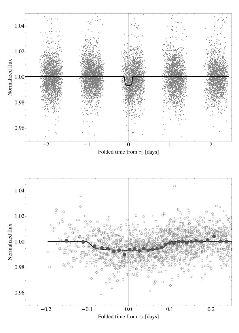
Figure 2.— Unbinned light curve of HAT-P-31 including all 8436 instrumental $I_{C}$ band 5.5 minute cadence measurements obtained with the HAT-5 and HAT-8 telescopes of HATNet (see the text for details), and folded with the period $P=5.005425$ days resulting from the global fit described in Section 3). The solid line shows our transit model fit to the light curve (Section 3.2). The bottom panel shows a zoomed-in view of the transit, the filled circles show the light curve binned in phase with a bin-size of 50 points.

Standard photometric procedures were used to calibrate the HATNet frames and then these calibrated images were subjected to star detection and astrometry, as described in Pál & Bakos (2006). Aperture photometry was performed on each image at the stellar centroids derived from the Two Micron All Sky Survey (2MASS; Skrutskie et al., 2006) catalog and the individual astrometric solutions. The resulting light curves were decorrelated (cleaned of trends) using the External Parameter Decorrelation (EPD; see Bakos et al., 2010) technique in “constant” mode and the Trend Filtering Algorithm (TFA; see Kovács et al., 2005).

The light curves were searched for transits using the Box-fitting Least-Squares (BLS; Kovács et al., 2002) method. We detected a significant signal in the light curve of GSC 2099-00908 (also known as 2MASS 18060904+2625359; $\alpha=18^{\mathrm{h}}06^{\mathrm{m}}09.00{\mathrm{s}}$, $\delta=+26{\arcdeg}25{\arcmin}36.0{\arcsec}$; J2000; V=11.660 Droege et al., 2006), with an apparent depth of $\sim 5.1$ mmag, and a period of $P=5.0050$ days. The BLS periodogram is shown in Figure 1. The drop in brightness had a first-to-last-contact duration, relative to the total period, of $q=0.0432\pm 0.0038$, corresponding to a total duration of $5.187\pm 0.462$ hr. Due to the lack of follow-up photometry, the HATNet photometry was re-processed with more computationally expensive reconstructive TFA, as discussed in §2 and shown in Figure 2. The EPD and reconstructive TFA corrected photometry is provided in Table 2.1.

Table 1HATNet differential photometry of HAT-P-31

BJD	Mag (EPD)	Mag (TFA)	$\sigma_{\rm Mag}$
(2,400,000$+$)
$54178.0007000$	$11.4164$	$11.4203$	$0.0075$
$54178.0045362$	$11.4267$	$11.4273$	$0.0073$
$54178.0083829$	$11.4250$	$11.4317$	$0.0075$
$54178.0122220$	$11.4177$	$11.4275$	$0.0069$
$54178.0160619$	$11.4244$	$11.4220$	$0.0072$
⋮	⋮	⋮	⋮

[-1.5ex]

Note. — This table is available in a machine-readable form in the online journal. A portion is shown here for guidance regarding its form and content.

2.2. Reconnaissance Spectroscopy

High-resolution, low-S/N reconnaissance spectra were obtained for HAT-P-31 using the Tillinghast Reflector Echelle Spectrograph (TRES; Fűrész et al., 2008) on the 1.5 m Tillinghast Reflector at FLWO, and the echelle spectrograph on the Australian National University (ANU) 2.3 m telescope at Siding Spring Observatory (SSO) in Australia. The two TRES spectra of HAT-P-31 were obtained, reduced and analyzed to measure the stellar effective temperature, surface gravity, projected rotation velocity, and RV via cross-correlation against a library of synthetic template spectra. The reduction and analysis procedure has been described by Quinn et al. (2010) and Buchhave et al. (2010). A total of 14 spectra of HAT-P-31 were obtained with the ANU 2.3 m telescope. These data were collected, reduced and analyzed to measure the RV via cross-correlation against the spectrum of a RV standard star HD 223311 following the procedure described by Béky et al. (2011). The resulting measurements from TRES and the ANU 2.3 m telescope are given in Table 2.

These observations revealed no detectable RV variation at the 1 $\rm km\,s^{-1}$ precision of the observations. Additionally the spectra are consistent with a single, slowly-rotating, dwarf star.

Table 2 Summary of reconnaissance spectroscopy observations of HAT-P-31

Instrument	Date	Number of	$T_{\rm eff\star}$	$\log(g_{*}\,[\mathrm{cgs}])$	$v\sin{i}$	$\gamma_{\rm RV}$
		Spectra	[K]		[$\rm km\,s^{-1}$]	[$\rm km\,s^{-1}$]
TRES	2009 Jul 05	1	$6000$	$4.0$	$4$	$-2.342$
TRES	2009 Jul 07	1	$6000$	$4.0$	$4$	$-2.300$
ANU 2.3 m	2009 Jul 14	5	$\cdots$	$\cdots$	$\cdots$	$-8.07\pm 0.35$
ANU 2.3 m	2009 Jul 17	5	$\cdots$	$\cdots$	$\cdots$	$-7.13\pm 0.40$
ANU 2.3 m	2009 Jul 18	2	$\cdots$	$\cdots$	$\cdots$	$-7.64\pm 0.44$
ANU 2.3 m	2009 Jul 19	2	$\cdots$	$\cdots$	$\cdots$	$-7.54\pm 0.49$

2.3. High Resolution, High S/N Spectroscopy

We proceeded with the follow-up of this candidate by obtaining high-resolution, high-S/N spectra to characterize the RV variations, and to refine the determination of the stellar parameters. For this we used the HIRES instrument (Vogt et al., 1994) with the iodine-cell (Marcy & Butler, 1992) on the Keck I telescope, the High-Dispersion Spectrograph (HDS; Noguchi et al., 2002) with the iodine-cell (Sato et al., 2002) on the Subaru telescope, and the FIbr-fed Échelle Spectrograph (FIES) on the 2.5 m Nordic Optical Telescope (NOT; Djupvik & Andersen, 2010). Table 2.3 summarizes the observations. The table also provides references for the methods used to reduce the data to relative RVs in the Solar System barycentric frame. The resulting RV measurements and their uncertainties are listed in Table 2.3. The different instrumental uncertainties arise from different slit widths, exposure times and seeing conditions. The period-folded data, along with our best fit described below in Section 3, are displayed in Figure 3.

Table 3 Summary of high resolution, high S/N spectroscopy observations of HAT-P-31

Instrument	Date	Number of	Reduction
	Range	RV obs.	Reference
HDS	2009 Aug 08 – 2010 May 24	25	1
HIRES	2010 Feb 24 – 2010 Jul 3	9	2
FIES	2009 Oct 6 – 2009 Oct 11	6	3

References. — 1: Sato et al. (2005), 2: Butler et al. (1996), 3: Buchhave et al. (2010)

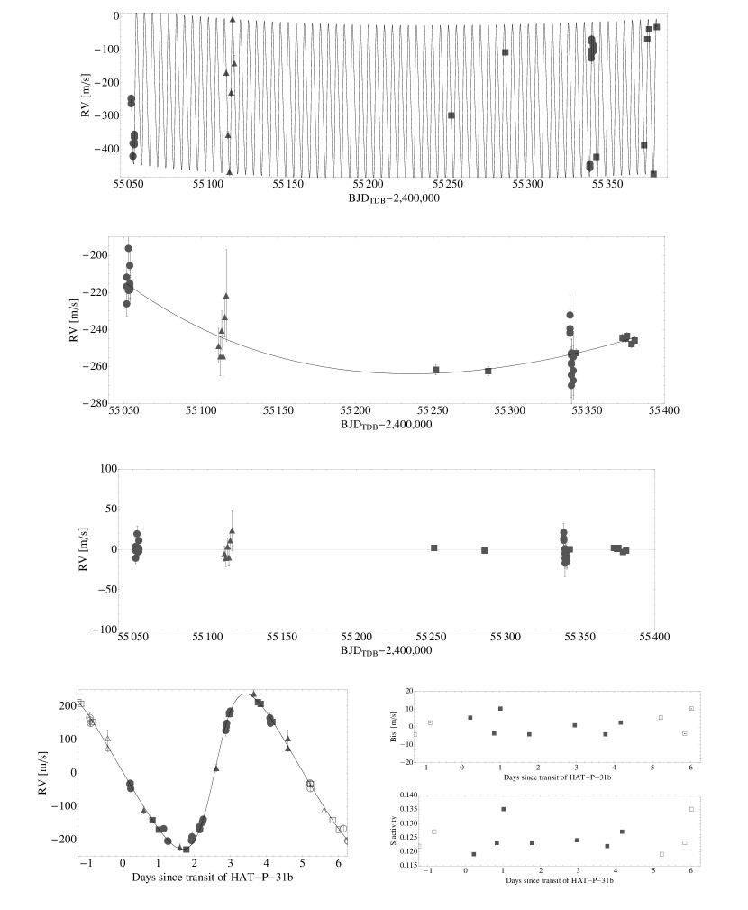
Figure 3.— First Row: Keck/HIRES (squares), Subaru (circles) and FIES (triangles) RV measurements for HAT-P-31, along with our best-fit 2-planet model (see Table 7). The center-of-mass velocity has been subtracted. Second Row: Same as top panel except the RV model of the inner planet has been subtracted from the data and the model, revealing the orbit of the outer planet. The $\chi^{2}$ of the best-fit 2-planet model is 34.8 for 39 data points (rms of 9.60 m/s) indicating a stellar jitter at or below the measurements errors. Third Row: Residuals from our best-fit model. Lower left: RV measurements phased to the orbital periods of the inner planet (left). The quadratic trend has been removed. Lower right: Upper panel shows the bisector spans (BS), with the mean value subtracted, phased at the period of the inner planet. Lower panel shows relative chromospheric activity index $S$ measured from the Keck spectra, phased at the period of the inner planet. Note the different vertical scales of the panels. Observations shown twice are represented with open symbols.

One false-alarm possibility is that the observed radial velocities are not induced by a planetary companion, but are instead caused by distortions in the spectral line profiles due to contamination from a nearby unresolved eclipsing binary. This hypothesis may be interrogated by examining the spectral line profiles for contamination from a nearby unresolved eclipsing binary (Queloz et al., 2001; Torres et al., 2007). A bisector analysis based on the Keck spectra was performed as described in §5 of Bakos et al. (2007). The resulting bisector spans, plotted in Figure 3, show no significant variation, and are not correlated with the RVs, indicating that this is a real TEP system.

In the same figure, one can also see the S index (Vaughan, Preston & Wilson, 1978), which is a quantitative measure of the chromospheric activity of the star derived from the flux in the cores of the Ca II H and K lines (Isaacson & Fischer, 2010). Following Noyes et al. (1984) we find that HAT-P-31 has an activity index $\log R^{\prime}_{\rm HK}=-5.312$, implying that this is a very inactive star.

Table 4 Relative radial velocities, bisector spans, and activity index measurements of HAT-P-31.

Note. — For the iodine-free template exposures there is no RV measurement, but the BS and S index can still be determined.

3. Analysis

The analysis of the HAT-P-31 system, including determinations of the properties of the host star and planet, was carried out in a similar fashion to previous HATNet discoveries (e.g. Bakos et al., 2010). Below, we briefly summarize the procedure and the results for the HAT-P-31b system.

3.1. Properties of the Parent Star

Stellar atmospheric parameters were measured from our template Keck/HIRES spectrum using the Spectroscopy Made Easy (SME; Valenti & Piskunov, 1996) analysis package, and the atomic line database of Valenti & Fischer (2005). SME yielded the following values and uncertainties: effective temperature $T_{\rm eff\star}=6065\pm 100$ K, metallicity $\rm[Fe/H]=+0.15\pm 0.08$ dex, and stellar surface gravity $\log{g_{\star}}=4.26_{-0.13}^{+0.11}$ (cgs), projected rotational velocity $v\sin{i}=0.5\pm 0.6\,\rm km\,s^{-1}$.

The above atmospheric parameters are then combined with the Yonsei-Yale (YY) (Yi et al., 2001) series of stellar evolution models to determine other parameters such as the stellar mass, radius and age. The results are listed in Table 5. We find that the star has a mass and radius of $M_{\star}\ =1.218_{-0.063}^{+0.089}$ $M_{\sun}$ and $R_{\star}\ =1.36_{-0.18}^{+0.27}$ $R_{\sun}$, and an estimated age of $3.17_{-1.11}^{+0.70}$ Gyr.

For previous HATNet planets (e.g. Bakos et al., 2010) we used the normalized semimajor axis, $a/R_{\star}$  which is closely related to $\rho_{\star}$, the mean stellar density, and is determined from the analysis of the light curves and RV curves, to obtain an improved estimate of $\log{g_{\star}}$, which is then held fixed in a second SME iteration. In this case, because we only have the relatively low-precision HATNet light curve, $a/R_{\star}$ is poorly constrained, and we instead opt to use the SME determination of $\log{g_{\star}}$ rather than $a/R_{\star}$ as a luminosity indicator. Figure 4 shows the location of the star in a diagram of $\log{g_{\star}}$ versus $T_{\rm eff\star}$, together with the model isochrones. For comparison we also show the relatively poor constraint on $\log{g_{\star}}$ that is imposed by $a/R_{\star}$.

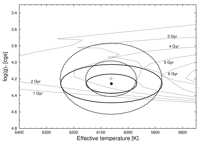
Figure 4.— Model isochrones from Yi et al. (2001) for the measured metallicity of HAT-P-31, $\rm[Fe/H]$= $0.15$, and ages from 1 to 14 Gyr in steps of 1 Gyr (gray-scale lines, left to right). The adopted values of $T_{\rm eff\star}$ and $\log{g_{\star}}$  determined from the SME analysis, are shown together with their 1-$\sigma$ and 2-$\sigma$ confidence ellipsoids (filled circle, and bold solid lines). The less-tight 1-$\sigma$ and 2-$\sigma$ constraints imposed by $a/R_{\star}$ are also shown (open triangle, and bold dotted lines).

As an additional check on the stellar evolution modeling, we note that HAT-P-31 has a measured near-infrared color of $J-K=0.364\pm 0.034$, which we have taken from 2MASS (Skrutskie et al., 2006) using the Carpenter (2001) transformation to the ESO photometric system. This is within 2-$\sigma$ of the predicted value from the isochrones of $J-K=0.31\pm 0.11$. The distance listed in Table 5 is calculated by comparing the observed $K$ magnitude (taken from 2MASS and transformed to ESO) to the absolute $K$ magnitude from the stellar models.

Table 5 Stellar parameters for HAT-P-31

Parameter	Value	Source
Spectroscopic properties
$T_{\rm eff\star}$ [K]	$6065\pm 100$	SME
$\rm[Fe/H]$	$0.15\pm 0.08$	SME
$v\sin{i}$ [$\rm km\,s^{-1}$]	$0.5\pm 0.6$	SME
$v_{\rm mac}$ [$\rm km\,s^{-1}$]	$4.47$	SME
$v_{\rm mic}$ [$\rm km\,s^{-1}$]	$0.85$	SME
$\gamma_{\rm RV}$ [$\rm km\,s^{-1}$]	$-2.40\pm 0.03$	TRES
Photometric properties
$V$ [mag]	11.660	TASS
$V\!-\!I_{C}$ [mag]	$0.67\pm 0.17$	TASS
$J$ [mag]	$10.423\pm 0.023$	2MASS
$H$ [mag]	$10.128\pm 0.027$	2MASS
$K_{s}$ [mag]	$10.083\pm 0.021$	2MASS
Derived properties
$M_{\star}$ [$M_{\sun}$]	$1.218_{-0.063}^{+0.089}$	YY+SME
$R_{\star}$ [$R_{\sun}$]	$1.36_{-0.18}^{+0.27}$	YY+SME
$\log(g_{*}\,[\mathrm{cgs}])$	$4.26_{-0.13}^{+0.11}$	YY+SME
$L_{\star}$ [$L_{\sun}$]	$2.23_{-0.58}^{+1.01}$	YY+SME
$M_{V}$ [mag]	$3.91_{-0.41}^{+0.34}$	YY+SME
$M_{K}$ [mag,ESO]	$2.64\pm 0.30$	YY+SME
Age [Gyr]	$3.17_{-1.11}^{+0.70}$	YY+SME
Distance [pc]	$354_{-51}^{+74}$	YY+SME

3.2. Global Modeling of the Data

3.2.1 Photometry

In previous HATNet papers, we have used a simplified model for the transit light curve of the HATNet data. For HAT-P-31, no precise photometry exists and thus we fit the HATNet data using a more sophisticated quadratic limb darkening Mandel & Agol (2002) algorithm with limb darkening coefficients interpolated from the tables by Claret (2004). One caveat is that the instrumental blending factor, $B_{\mathrm{inst}}$, is unknown as discussed earlier in §2. We point out that experience with previous HATNet planets suggests $B_{\mathrm{inst}}$ is within 2-$\sigma$ of unity for light curves processed using reconstructive TFA in all cases and thus can be accounted for by conservatively doubling the uncertainties on $p$ and $R_{P}$. Further support for a $B_{\mathrm{inst}}$ factor not greatly different from unity come from the fact HAT-P-31 is fairly isolated and there are no neighbors in 2MASS or a DSS image which contribute significant flux to the HATNet aperture.

Due to the low-precision photometry, the stellar density cannot be determined to high precision using the method of Seager & Mallén-Ornelas (2003) and in fact spectroscopic estimates were found to be more precise. However, we can reverse this well-known trick by implementing a Bayesian prior in our fitting process for the stellar density.

We use the spectroscopically determined stellar density from §3.1 as a prior in our fits. Since the period of the transiting planet is well constrained for even low signal-to-noise photometry, reasonably precise estimates for $P_{b}$ and $\rho_{*}$ are possible. With these two constrained, $(a_{b}/R_{*})$ is therefore also constrained. The transit light curve is essentially characterized by four parameters, $\tau_{b}$, $\delta_{b}$, $b_{b}$ and $(a_{b}/R_{*})$ and thus one of these parameters is constrained by the combination of the transit times and the stellar density prior alone.

The photometry which is fitted in the global modeling is corrected for instrumental systematics through the EPD and reconstructive TFA correction procedures prior to performing the fit (see § 2.1 and Bakos et al. (2010) for details).

3.2.2 Radial velocities

For the radial velocity fits, we found a single planet fit gave a very poor fit to the observations ($\chi^{2}=204.2$ for 40 RV points) and quickly appreciated some kind of second signal was present. Exploring different models, such as Trojan offsets, polynomial time trends and outer companions, (see Table 6 for comparison), we found that an eccentric transiting planet with a quadratic trend in the RVs was the preferred model. The pivot point ($t_{\mathrm{pivot}}$) of the polynomial models, including the drift and quadratic trends, was selected to be the weighted mean of the radial velocity time stamps.

The most likely physical explanation for a quadratic trend is a third body in the system, described by a Keplerian model. Indeed, the Keplerian model provides an improved $\chi^{2}$ for a circular orbit and then again for an eccentric orbit but the extra degrees of freedom penalize our model selection criterion. We also found that these models were highly unconstrained and convergence in the associated fits was unsatisfactory. An illustration of the lack of convergence is shown in Figure 6. Therefore, we will adopt the quadratic model in our final reported parameters in Table 7.

The quadratic model may be used to infer some physical parameters of the third planet. To make some meaningful progress, we will assume the outer planet is on a circular orbit. One may compare the quadratic and Keplerian model descriptions via:

$$\mathrm{RV}_{\mathrm{quad}}^{c} =\gamma^{\prime}+\dot{\gamma}(t-t_{\mathrm{pivot}})+0.5\ddot{\gamma}(t-t_{\mathrm{pivot}})^{2}$$ (1)

$$\mathrm{RV}_{\mathrm{Kep}}^{c} =\gamma^{\prime}-K_{c}\sin\Bigg{(}\frac{2\pi(t-\tau_{c})}{P_{c}}\Bigg{)}$$ (2)

By differentiating both expressions and solving for the time when the signals are minimized, one may write:

$$\tau_{c}+\frac{P_{c}}{4} =\frac{-\dot{\gamma}+\ddot{\gamma}t_{\mathrm{pivot}}}{\ddot{\gamma}}$$ (3)

Differentiating both RV models with respect to time twice and evaluating at the moment when both signals are minimized, yields:

$$\frac{K_{c}}{P_{c}^{2}} =\frac{\ddot{\gamma}}{4\pi^{2}}$$ (4)

Equations 3&4 may therefore be used to determine some information about HAT-P-31c.

To evaluate the statistical significance of HAT-P-31c, we performed an F-test between the one-planet and two-planet models. In both cases, HAT-P-31b is assumed to maintain non-zero orbital eccentricity. Assuming HAT-P-31c is on a circular orbit, the false-alarm-probability (FAP) from an F-test is $3.0\times 10^{-12}$, or 7.0-$\sigma$. Assuming HAT-P-31c is on an eccentric orbit requires 2 more degrees of freedom and thus reduces the FAP to $1.3\times 10^{-10}$, or 6.4-$\sigma$. From a statistical perspective then, the presence of HAT-P-31c is highly secure. We point out this determination of course assumes purely Gaussian uncertainties and no outlier measurements.

Table 6 Comparison of RV models attempted for HAT-P-31

Model	$\chi^{2}$	BIC
Circular Planet	3714.9	3729.6
Eccentric Planet	204.2	226.3
Eccentric Planet + Drift	159.6	185.5
Eccentric Planet + Trojan	191.1	216.9
Eccentric Planet + Drift + Trojan	113.2	142.7
Eccentric Planet + Drift + Quadratic	33.9	63.4
Eccentric Planet + Circular Planet	33.6	66.8
Eccentric Planet + Eccentric Planet	33.2	73.8

3.2.3 Fitting algorithm

We utilize a Metropolis-Hastings Markov Chain Monte Carlo (MCMC) algorithm to globally fit the data, including the stellar density prior (our routine is described in Kipping & Bakos (2011)). To ensure the parameter space is fully explored, we used 5 independent MCMC fits which stop once $1.25\times 10^{5}$ trials have been accepted and burn-out the first 20%. This leaves us with a total of $5\times 10^{5}$ points for the posterior distributions. At the end of the fit, a more aggressive downhill simplex $\chi^{2}$ minimization is used, for which the final solution is used for Figures 2&3.

There were 14 free parameters in the global fit: {$\tau_{b}$, $p_{b}^{2}$, $[\tilde{T}_{1}]_{b}$, $b_{b}$, $P_{b}$, $e_{b}\sin\omega_{b}$, $e_{b}\cos\omega_{b}$, $\gamma_{\mathrm{Keck}}$, $\gamma_{\mathrm{FIES}}$, $\gamma_{\mathrm{Subaru}}$, $K_{b}$, $\dot{\gamma}$, $\ddot{\gamma}$, OOT}, which we elaborate on here. $\tau_{b}$ is the time of transit minimum (Kipping, 2011), frequently dubbed by the misnomer “mid-transit time”. $p_{b}^{2}$ is the ratio-of-radii squared and $P_{b}$ is the orbital period. $[\tilde{T}_{1}]_{b}$ is the “one-term” approximate equation (Kipping, 2010) for the transit duration between the instant when the center of the planet crosses the stellar limb to exiting under the same condition. $b_{b}$ is the impact parameter, defined as the sky-projected planet-star separation in units of the stellar radius at the instant of inferior conjunction. $e_{b}$ is the orbital eccentricity and $\omega_{b}$ is the associated position of pericenter. $\gamma$ terms relate to the instrumental offsets for the radial velocities. Similarly, OOT is the out-of-transit flux for the HATNet photometry. Finally, $K_{b}$ is the radial velocity semi-amplitude and $\dot{\gamma}$ (drift) & $\ddot{\gamma}$ (curl) are the first and second time derivatives of $\gamma$.

Final quoted results are the median of the marginalized posterior for each fitted parameter with 34.15% quantiles either side for the 1-$\sigma$ uncertainties (see Table 7). The uncertainties on $p$, $p^{2}$ and $R_{P}$ have been conservatively doubled for reasons described in §2. Histograms of the posterior distributions for the fitted parameters are provided in Figure 5. We find that the stellar jitter of this star is at or below the measurement uncertainties ($\sim 2$ m/s).

Table 7 provides estimates for some minimum limits on various parameters of interest relating to HAT-P-31c. These limits are determined by the known constraints on the minimum $P_{c}$. We determined this value by forcing a circular orbit Keplerian fit for planet c through the data, stepping through a range of periods from 1 year to 5 years in 1 day steps. The minimum limit on $P_{c}$ is defined as when $\Delta\chi^{2}=1$, relative to the quadratic trend fit, occurring at 2.8 years.

Table 7 Global fit results for HAT-P-31

Parameter	Value
Fitted Parameters
$P_{b}$ [days]	$5.005425_{-0.000092}^{+0.000091}$
$\tau_{b}$ [BJDTDB - 2,450,000]	$4320.8866_{-0.0053}^{+0.0051}$
$[\tilde{T}_{1}]_{b}$ [s]	$16300_{-1000}^{+1000}$
$p_{b}^{2}$ [%]	$0.65_{-0.12}^{+0.18}$
$b_{b}$	$0.57_{-0.31}^{+0.23}$
OOT	$1.00061_{-0.00016}^{+0.00016}$
$K_{b}$ [ms-1]	$232.5_{-1.1}^{+1.1}$
$e_{b}\sin\omega_{b}$	$-0.2442_{-0.0043}^{+0.0043}$
$e_{b}\cos\omega_{b}$	$0.0185_{-0.0079}^{+0.0080}$
$\gamma_{\mathrm{Keck}}$ [ms-1]	$-29.0_{-1.4}^{+1.4}$
$\gamma_{\mathrm{Subaru}}$ [ms-1]	$18.8_{-3.1}^{+3.1}$
$\gamma_{\mathrm{FIES}}$ [ms-1]	$92.7_{-5.6}^{+5.6}$
$\dot{\gamma}$ [ms-1day-1]	$0.141_{-0.025}^{+0.025}$
$\ddot{\gamma}$ [ms-1day-2]	$0.00226_{-0.00021}^{+0.00021}$
SME Derived Quantities
$u_{1}$	$0.2078^{*}$
$u_{2}$	$0.3550^{*}$
$\rho_{*}$ [g cm-3]	$0.69_{-0.26}^{+0.34}$
HAT-P-31b Derived Properties
$\Psi_{b}$	$0.4737_{-0.0064}^{+0.0065}$
$e_{b}$	$0.2450_{-0.0045}^{+0.0045}$
$\omega_{b}$ [∘]	$274.3_{-1.8}^{+1.8}$
$\log(g_{b}\,[\mathrm{cgs}])$	$3.61_{-0.32}^{+0.15}$
$(a_{b}/R_{*})$	$8.9_{-2.3}^{+1.4}$
$i_{b}$ [∘]	$87.1_{-2.7}^{+1.8}$
$[T_{1,4}]_{b}$ [s]	$18500_{-1200}^{+1700}$
$[T_{2,3}]_{b}$ [s]	$14200_{-2400}^{+1300}$
$p_{b}$	$0.080_{-0.015}^{+0.022}$
$M_{b}$ [$M_{J}$]	$2.171_{-0.077}^{+0.105}$
$R_{b}$ [$R_{J}$]	$1.07_{-0.16}^{+0.24}$
Corr($R_{b}$,$M_{b}$)	0.795
$\rho_{b}$ [g cm-3]	$2.18_{-0.93}^{+1.24}$
$a_{b}$ [AU]	$0.055_{-0.015}^{+0.015}$
$[T_{\mathrm{eq}}]_{b}$ [K]	$1450_{-110}^{+230}$
$\Theta$	$0.190_{-0.056}^{+0.036}$
$F_{\mathrm{peri}}$ [$10^{9}$$\rm erg\,s^{-1}\,cm^{-2}$]	$1.69_{-0.44}^{+1.39}$
$F_{\mathrm{ap}}$ [$10^{9}$$\rm erg\,s^{-1}\,cm^{-2}$]	$0.62_{-0.16}^{+0.51}$
$\langle F\rangle$ [$10^{9}$$\rm erg\,s^{-1}\,cm^{-2}$]	$0.99_{-0.26}^{+0.82}$
HAT-P-31c Derived Quantities
$\tau_{c}+0.25P_{c}$ [BJDTDB - 2,450,000]	$5254.9_{-6.8}^{+7.4}$
$K_{c}P_{c}^{-2}$ [ms-1day-2]	$7.64_{-0.70}^{+0.71}$
$P_{c}$ [years]	$\geq 2.8$
$K_{c}$ [ms-1]	$\geq 60$
$M_{c}$ [$M_{J}$]	$\geq 3.4$

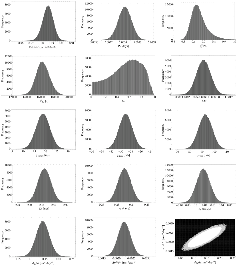
Figure 5.— Posterior distributions of the fitted parameters used in the global fits (described in §3.2) from our global fits. Histograms computed from $5\times 10^{5}$ MCMC trials. Bottom-right panel shows joint-posterior of the radial velocity drift and curl, with white denoting the 2-$\sigma$ region of confidence and gray the 3-$\sigma$.

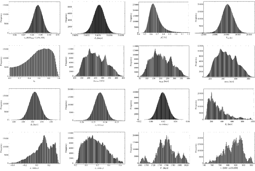
Figure 6.— Top row: Marginalized posterior distributions for $K_{c}$ and $P_{c}$ when we attempted to fit for a second Keplerian signal, instead of a quadratic trend. The multi-modal nature of these histograms reflect the unconverged nature of the fits. Bottom row: History of the MCMC trials for the same parameters and the same fit. Each continuous line represents one of the ten independent MCMC chains. The lines clearly illustrate the inability of the current data to converge upon a solution for HAT-P-31c.

4. Discussion

4.1. Physical Properties of HAT-P-31b&c

HAT-P-31b is a $2.17$ $M_{J}$ hot-Jupiter transiting the host star once every $5.005$ days. Due to the lack of follow-up photometry obtained for this object (as a consequence of the nearly integer orbital period), we have only HATNet photometry, which is of lower signal-to-noise than dedicated follow-up. This fact, combined with our choice to double all uncertainties on depth related transit terms, leads to a large uncertainty on the planetary radius of $R_{b}=1.07_{-0.32}^{+0.48}$ $R_{J}$, consistent with many other hot-Jupiter objects (see http://exoplanet.eu).

High-precision radial velocities also indicate the presence of an outer body, HAT-P-31c, found through an induced quadratic trend in the RV residuals. Keplerian fits are unable to convincingly distinguish between a circular or eccentric orbit for this object. HAT-P-31c has a minimum mass of $M_{c}\geq 3.4$ $M_{J}$ and eccentric orbit solutions significantly increase this figure. It is unclear whether HAT-P-31c is a brown dwarf or a “planet”, and future work will be needed to determine this.

4.2. Orbital Stability

4.2.1 Circular fit for HAT-P-31c

Here we discuss our procedure to test the dynamical stability of two possible orbital configurations. It should be noted that the eccentricity of HAT-P-31b is highly secure but the eccentricity of HAT-P-31c remains unclear. For this reason, we repeat our simulations assuming both a circular and eccentric orbit for HAT-P-31c, beginning with the former. We utilize the Systemic Console (Meschiari et al., 2009) for this purpose assuming a coplanar configuration. Employing the Gragg-Bulirsch-Stoer integrator, orbital evolution was computed for 250,000 years for the HAT-P-31 system (see Figure 7).

We first consider the circular case. The orbital period and mass of HAT-P-31c are non-convergent parameters and so we can only provide an orbital solution which gives a good fit to the data, but is not necessarily unique. To this end, we proceeded to input HAT-P-31c with $P_{c}=4.86$ years and $M_{c}=13.0$ $M_{J}$, corresponding to the solution presented in Table 6. This test revealed minor evolution over the course of our simulations, indicating a stable and essentially static configuration.

4.2.2 Eccentric fit for HAT-P-31c

To test the eccentric fit, we again used the lowest $\chi^{2}$ solution presented earlier in Table 6, corresponding to $P_{c}=4.82$ years and $e_{c}=0.285$. We found that the system was also stable over 250,000 years (see Figure 7). However, the simulations do show the eccentricity of planet b varying sinusoidally over a timescale of $\sim$125,000 years with an amplitude of $\sim 0.01$. The eccentricity of planet c also varies in anti-phase but with a much smaller amplitude. The eccentric evolution shows faster apsidal precession for planet b, but this is unlikely to be observable through changes in the transit duration. We estimate the duration will change by 0.2 s over 10 years (corresponding to $\Delta\omega_{b}=0.027^{\circ}$) using the expressions of Kipping (2010).

The orbital period and semi-major axes of both bodies were stable over the 250,000 years of integration considered here.

4.2.3 Habitable-zone bodies

We tried adding a habitable-zone Earth-mass planet on a circular orbit into the system and testing stability. One may argue that the probable history of this system involved the inwards migration of HAT-P-31b and that this migration through the inner protoplanetary disk would essentially eliminate the possibility of an Earth-like planet forming in the habitable-zone. However, Fogg & Nelson (2007) have shown that this not necessarily true. In their simulations, it is found that $>60$% of the solid disk survives, including planetesimals and protoplanets, by being scattered by the giant planet into external orbits where dynamical friction is strong and terrestrial planet formation is able to resume. In one simulation, a planet of $2\,M_{\oplus}$ formed in the habitable-zone after a hot-Jupiter passed through and its orbit stabilized at 0.1 AU.

For a planet to receive the same insolation as the Earth, we estimate $P=604$ days. For our circular orbit solution of HAT-P-31c, the habitable-zone Earth-mass planet is stable for over 100,000 years. For our eccentric orbit solution, the Earth-like planet is summarily ejected in less than 1000 years.

Figure 7.— Two possible realizations for the orbital evolution of planets HAT-P-31b and c. The solid lines show the evolution starting from an eccentric orbit solution for HAT-P-31c. The dashed lines show the evolution starting from a circular orbit solution for HAT-P-31c.

4.3. Circularization Timescale

Due to the poor constraints on the planetary radius, there is a great deal of uncertainty in the circularization timescale ($\tau_{\mathrm{circ}}$) for HAT-P-31b. Nevertheless, using the equations of Adams & Laughlin (2006), we used the MCMC results to compute the posterior distribution of $\tau_{\mathrm{circ}}$. We find that the age of HAT-P-31 is equal to $24_{-15}^{+122}$ circularization timescales, assuming $Q_{P}=10^{5}$. This indicates that we currently have insufficient data to assess whether the observed eccentricity is anomalous or not. Improved radius constraints will certainly aid in this calculation and may lend or detract credence to the hypothesis of eccentricity pumping of the inner planet by HAT-P-31c.

References

- Adams & Laughlin (2006) Adams, F. C. & Laughlin, G., 2006, ApJ, 649, 1004
- Agol et al. (2005) Agol, E., Steffen, J., Sari, R., & Clarkson, W. 2005, MNRAS, 359, 567
- Bakos et al. (2004) Bakos, G. Á., Noyes, R. W., Kovács, G., Stanek, K. Z., Sasselov, D. D., & Domsa, I. 2004, PASP, 116, 266
- Bakos et al. (2007) Bakos, G. Á., et al. 2007, ApJ, 670, 826
- Bakos et al. (2010) Bakos, G. Á., et al. 2010, ApJ, 710, 1724
- Béky et al. (2011) Béky, B., et al. 2011, ApJ, submitted, arXiv:1101.3511
- Buchhave et al. (2010) Buchhave, L. A., et al. 2010, ApJ, submitted, arXiv:1005.2009
- Butler et al. (1996) Butler, R. P. et al. 1996, PASP, 108, 500
- Carpenter (2001) Carpenter, J. M. 2001, AJ, 121, 2851
- Claret (2004) Claret, A. 2004, A&A, 428, 1001
- Djupvik & Andersen (2010) Djupvik, A. A., & Andersen, J. 2010, in Highlights in Spanish Astrophysics V, ed. J. M. Diego et al. (Berlin: Springer), 211
- Droege et al. (2006) Droege, T. F., Richmond, M. W., & Sallman, M. 2006, PASP, 118, 1666
- Fogg & Nelson (2007) Fogg, M. J. & Nelson, R. P. 2007, A&A, 461, 1195
- Fűrész et al. (2008) Fűrész, G. 2008 Ph.D. thesis, University of Szeged, Hungary
- Hansen & Barman (2007) Hansen, B. M. S., & Barman, T. 2007, ApJ, 671, 861
- Isaacson & Fischer (2010) Isaacson, H., & Fischer, D. 2010, ApJ, 725, 875
- Johnson et al. (2011) Johnson, J. A. et al., 2011, ApJ, submitted
- Kipping (2009a) Kipping, D. M. 2009a, MNRAS, 392, 181
- Kipping (2009b) Kipping, D. M. 2009b, MNRAS, 396, 1797
- Kipping (2010) Kipping, D. M. 2010, MNRAS, 407, 301
- Kipping (2011) Kipping, D. M. 2011, PhD thesis, University College London (astro-ph:1105.3189)
- Kipping & Bakos (2011) Kipping, D. M. & Bakos, G. A. 2011, ApJ, 730, 50
- Kovács et al. (2002) Kovács, G., Zucker, S., & Mazeh, T. 2002, A&A, 391, 369
- Kovács et al. (2005) Kovács, G., Bakos, G. Á., & Noyes, R. W. 2005, MNRAS, 356, 557
- Kovács et al. (2010) Kovács, G., et al. 2010, ApJ, submitted, arXiv:1005.5300
- Latham et al. (2009) Latham, D. W., et al. 2009, ApJ, 704, 1107
- Liddle (2007) Liddle, A. R. 2007, MNRAS, 377, L74
- Noyes et al. (1984) Noyes, R. W., Hartmann, L. W., Baliunas, S. L., Duncan, D. K., & Vaughan, A. H. 1984, ApJ, 279, 763
- Pál & Bakos (2006) Pál, A., & Bakos, G. Á. 2006, PASP, 118, 1474
- Mandel & Agol (2002) Mandel, K., & Agol, E. 2002, ApJ, 580, L171
- Marcy & Butler (1992) Marcy, G. W., & Butler, R. P. 1992, PASP, 104, 270
- Meschiari et al. (2009) Meschiari, S., Wolf, A. S., Rivera, E., Laughlin, G., Vogt, S. & Butler, P. 2009, PASP, 121, 1016
- Noguchi et al. (2002) Noguchi, N., et al. 2002, PASJ, 54, 819
- Queloz et al. (2001) Queloz, D., et al. 2001, A&A, 379, 279
- Quinn et al. (2010) Quinn, S. N., et al. 2010, ApJ, submitted, arXiv:1008.3565
- Sato et al. (2002) Sato, B., Kambe, E., Takeda, Y., Izumiura, H., & Ando, H. 2002, PASJ, 54, 873
- Sato et al. (2005) Sato, B., et al. 2005, ApJ, 633, 465
- Schwarz (1978) Schwarz, G. 1978, The Annals of Statistics, 6, 461
- Seager & Mallén-Ornelas (2003) Seager, S. & Mallén-Ornelas, G., 2003, ApJ, 585, 1083
- Skrutskie et al. (2006) Skrutskie, M. F., et al. 2006, AJ, 131, 1163
- Tinetti et al. (2007) Tinetti, G. et al., 2007, Nature, 448, 163
- Torres et al. (2007) Torres, G. et al. 2007, ApJ, 666, 121
- Valenti & Piskunov (1996) Valenti, J. A., & Piskunov, N. 1996, A&AS, 118, 595
- Valenti & Fischer (2005) Valenti, J. A., & Fischer, D. A. 2005, ApJS, 159, 141
- Vogt et al. (1994) Vogt, S. S. et al. 1994, Proc. SPIE, 2198, 362
- Yi et al. (2001) Yi, S. K. et al. 2001, ApJS, 136, 417
- Vaughan, Preston & Wilson (1978) Vaughan, A. H., Preston, G. W., & Wilson, O. C. 1978, PASP, 90, 267
- Winn et al. (2011) Winn, J. N. et al. 2011, ApJ, 141, 63