Constructing Runge-Kutta Methods with the Use of Artificial Neural Networks

Abstract

A methodology that can generate the optimal coefficients of a numerical method with the use of an artificial neural network is presented in this work. The network can be designed to produce a finite difference algorithm that solves a specific system of ordinary differential equations numerically. The case we are examining here concerns an explicit two-stage Runge-Kutta method for the numerical solution of the two-body problem. Following the implementation of the network, the latter is trained to obtain the optimal values for the coefficients of the Runge-Kutta method. The comparison of the new method to others that are well known in the literature proves its efficiency and demonstrates the capability of the network to provide efficient algorithms for specific problems.

1 Introduction

The literature that involves solving ordinary or partial differential equations with the use of artificial neural networks is quite limited, but has grown significantly in the past decade. To name a few, Dissanayake et al. used a ”universal approximator” (see cybenko hornik ) to transform the numerical problem of solving partial differential equations to an unconstrained minimization problem of an objective function dissanayake . Meade et al. demonstrated feedforward neural networks that could approximate linear and nonlinear ordinary differential equations meade meade2 . Puffer et al. constructed cellular neural networks that were able to approximate the solution of various partial differential equations puffer . Lagaris et al. introduced a method for the solution of initial and boundary value problems, that consists of an invariable part, which satisfies by construction the initial/boundary conditions and an artificial neural network, which is trained to satisfy the differential equation lagaris . S. He et al. used feedforward neural networks to solve a special class of linear first-order partial differential equations he . The radial basis function (RBF) network architecture alexandridis has also been used for the solution of differential equations in jianyu , where Jianyu et al. demonstrated a method for solving linear ordinary differential equations based on multiquadric RBF networks. Ramuhalli et al. proposed an artificial neural network with an embedded finite-element model, for the solution of partial differential equations ramuhalli . Tsoulos et al. demonstrated a hybrid method for the solution of ordinary and partial differential equations, which employed neural networks, based on the use of grammatical evolution, periodically enhanced using a local optimization procedure tsoulos .

In all the aforementioned cases, the neural networks functioned as direct solvers of differential equations. In this work, however, we use the constructed neural network, not as a direct solver, but as a means to generate proper Runge-Kutta coefficients. In this aspect, there has been little relevant published material. For instance in tsitouras , Tsitouras constructs a multilayer feedforward neural network that uses input data associated with an initial value problem and trains the network to produce the solution of this problem as output data, thus generating (by construction of the network) coefficients for a predefined number of Runge-Kutta stages.

In this work we construct an artificial neural network that can generate the coefficients of two-stage Runge-Kutta methods. We consider the two-body problem, which is a typical case of an initial value problem where Runge-Kutta methods apply, and therefore the resulting method is specialized in solving it. The comparison shows that the new method is more efficient than the classical methods and thus proves the capability of the constructed neural network to create new Runge-Kutta methods.

The structure is as follows: in Sections 2 and 3 we present the basic theory for Runge-Kutta methods and Artificial Neural Networks respectively. In Section 4 we present the implementation of the neural network that applies to a two-stage Runge-Kutta method which solves the two-body problem numerically, while in Section 5 the derivation of the method is provided. In Section 6 we demonstrate the final results along with the comparison of the new method to other well-known methods and finally in Section 7 we reach some conclusions about this work.

2 Runge-Kutta methods

We consider a two-stage Runge-Kutta method to solve the first order initial value problem

$${\bf v}^{\prime}(t)=f(t,{\bf v})\,\,\,\mbox{and}\,\,\,{\bf v}(t_{0})={\bf v_{0}}$$ (1)

At each step of the integration interval, we approximate the solution of the initial value problem at $t_{n+1}$, where $t_{n+1}=t_{n}+h$. For the two-stage Runge-Kutta method, the approximate solution ${\bf v_{n+1}}$ is given by

$${\bf v_{n+1}}={\bf v_{n}}+h\,(b_{1}\,{\bf k_{1}}+b_{2}\,{\bf k_{2}})$$ (2)

where

$${\bf k_{1}}=f(t_{n},{\bf v_{n}})$$ (3)

$${\bf k_{2}}=f(t_{n}+c_{2}\,h,{\bf v_{n}}+h\,a_{21}\,{\bf k_{1}})$$ (4)

The coefficients for this set of methods can be presented by the Butcher tableau given below

$c_{2}$	$a_{21}$
	$b_{1}$	$b_{2}$

An explicit two-stage Runge-Kutta method can be of second algebraic order at most (see butcher ). In order for that to hold, the following conditions must be satisfied

$$b_{1}+b_{2}=1$$ (5)

$$b_{2}\,c_{2}=\frac{1}{2}$$ (6)

The extra condition that needs to be satisfied in order for the method to be consistent is

$$a_{21}=c_{2}$$ (7)

3 Artificial Neural Networks

An artificial neural network (ANN) is a network of interconnected artificial processing elements (called neurons) that co-operate with each other in order to solve specific problems. ANNs are inspired by the structure and functional aspects of biological nervous systems and therefore present a resemblance. Haykin in haykin defines an artificial neural network as ”a massively parallel distributed processor that has a natural propensity for storing experiential knowledge and making it available for use”. ANNs, similarly to brains, acquire knowledge through a learning process, which is called training. That knowledge is stored in the form of synaptic weights, whose values express the strength of the connection between two neurons.

There are many types of artificial neural networks, depending on the structure and the means of training. An ANN, in its simplest form, consists of a single neuron, in what we call the Perceptron model. The Perceptron is connected with a number of inputs: $x_{1}$, $x_{2}$, …, $x_{n}$. A weight corresponds to each of the neuron’s connections with the inputs and expresses the specific input’s significance to the calculation of the Perceptron’s output. Therefore, there is a number of weights equal to the number of inputs, with $w_{i}$ being the weight that corresponds to input $x_{i}$, and $w_{i}x_{i}$ being the combined weighted input. The neuron is also connected with a weight, which is not connected with any input and is called bias (symbolized by $b$). The weighted input data are essentially being mapped to an output value, through the transfer function of the neuron. The transfer function consists of the net input function and the activation function. The first function undertakes the task of combining the various weighted inputs into a scalar value. Typically, the summation function is used for this purpose, thus the net input in that case is described by the following expression

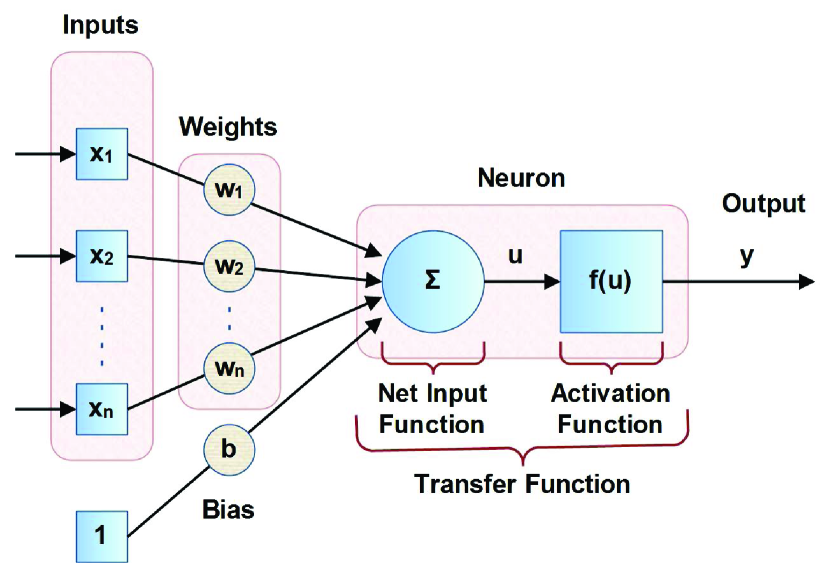
Figure 1: An artificial neuron (Perceptron)

$$u=\displaystyle\sum\limits_{i=1}^{n}w_{i}x_{i}+b$$ (8)

For ease of use, the bias can be treated as any other weight and be represented as $w_{0}$, with $x_{0}=1$, so the previous expression becomes

$$u=\displaystyle\sum\limits_{i=0}^{n}w_{i}x_{i}$$ (9)

The activation function receives the output $u$ of the net input function and produces its own output y (also known as the activation value of the neuron), which is a scalar value as well. The general form of the activation function is

$$y=f(u)$$ (10)

What is required of a neural network, such as the Perceptron, is the ability to learn. That means the ability to adjust its weights in order to be able to produce a specific set of output data for a specific set of input data. In the supervised type of learning (which is used to train the Perceptron and other types of neural networks), besides the input data, we provide the network with target data, which are the data that the output should ideally converge to, with the given set of input. The Perceptron uses an estimation of the error as a measure that expresses the divergence between the actual output and the target. In that sense, training is essentially the learning process of adjusting the synaptic weights, in order to minimize the aforementioned error. To achieve this, a gradient descent algorithm called delta rule is employed, also known as the Least Mean Square (LMS) method or the Widrow-Hoff rule, developed by Widrow and Hoff in widrow-hoff . The training process that uses the delta rule has the following steps:

1. Assign random values to the weights

2. Generate the output data for the set of the training input data

3. Calculate the error $E$, which is given by a norm of the differences between the target and the output data

4. Adjust the weights according to the following rule

   $$\Delta w_{i}=-\eta\frac{\partial E}{\partial w_{i}}=-\eta\frac{\partial E}{\partial u}\frac{\partial u}{\partial w_{i}}=\eta\delta x_{i}$$ (11)

   Where $\eta$ is a small positive constant, called learning step or learning rate, and $\delta$ (delta error) is equal to the following expression

   $$\delta=-\frac{\partial E}{\partial u}$$ (12)

5. Repeat from step 2, unless the error $E$ is less than a small predefined constant $\epsilon$ or the maximum number of iterations has been reached

With each iteration of the learning method, the weights are adjusted in such manner as to reduce the error. Notice that the correction $\Delta w_{i}$ of the weights is proportional to the negative of $\frac{\partial E}{\partial w_{i}}$, since the desired goal is the minimization of the error.

Strictly speaking, the Perceptron is not technically a network, since it consists of a single neuron. An actual network and the most common form of ANNs is the multilayer Perceptron (MLP), which falls in the general category of feedforward neural networks (FFNNs). Feedforward are the neural networks that contain no feedback connections, i.e. the connections do not form a loop, but are instead all directed towards the output of the network. A multilayer Perceptron consists of various layers, namely the input layer, the output layer, and one or more hidden layers. The hidden layers are not visible externally of the network, hence the ”hidden” property. Each of the layers consists of one or more neurons, except for the input layer, whose input nodes simply function as an entry point for the input data. Each layer is connected to the previous and the next layer, thus providing a pathway for the data to travel throughout the network. When a layer is connected to another, each neuron of the first layer is connected to every neuron of the second layer. In this way, the output of one layer becomes the input for the next one. Therefore, to calculate the output of the MLP, the data (either input data or activation values) are being propagated forward through the neural network.

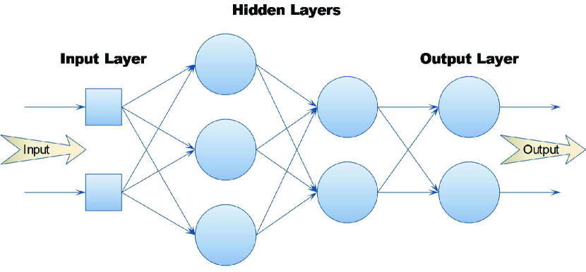
Figure 2: A typical multilayer Perceptron

To train the MLP, the backpropagation method is used. Backpropagation is a generalization of the delta rule that is used to train the Perceptron. The method, essentially, functions in the same way for each neuron of the MLP, as simple delta rule does for the Perceptron. The difference lies in the fact that, since the learning procedure requires the calculation of the $\delta$ error, the neurons that reside inside the hidden layers must be provided with the $\delta$ errors of the neurons of the next layer. For this reason, the $\delta$ errors are first calculated for the neurons of the output layer and are propagated backwards (hence the backpropagation term), all across the network. The procedure is the following:

1. Assign random values to the weights

2. Generate the activation values of each neuron, starting from the first hidden layer and continue until the output layer

3. Calculate the error $E$, which is given by a norm of the differences between the target and the output data

4. Calculate the $\delta$ errors of each neuron of the output layer, according to (12)

5. Calculate the $\delta$ errors of each neuron of the previous layer, according to

   $$\delta=f^{\prime}(u)\displaystyle\sum\limits_{i=1}^{M}w_{i}\delta_{i}$$ (13)

   Where $f(u)$ is the activation function of the neuron, $M$ is the number of the neurons in the next layer, and $\delta_{i}$ is the $\delta$ error of the $i$th neuron of the next layer

6. Repeat step 5 for the previous layer, until all $\delta$ errors for all the hidden layers have been calculated

7. Adjust the weights according to (11)

8. Repeat from step 2, unless the error $E$ is less than a small predefined constant $\epsilon$ or the maximum number of iterations has been reached

4 Implementation

We introduce a feedforward neural network that can generate the coefficients of two-stage Runge-Kutta methods, specifically designed to apply to the needs of the two-body problem. The two-body problem is described by the following system of equations

$$x^{\prime\prime}=-\frac{x}{r^{3}},\;y^{\prime\prime}=-\frac{y}{r^{3}},\;r=\sqrt{x^{2}+y^{2}}$$ (14)

whose analytical solution is given by

$$x=\cos{t},\quad y=\sin{t}$$ (15)

Since a Runge-Kutta method can only solve a system of first order ordinary differential equations, ${\bf v}$ according to the notation of equation (1), can be given by

$${\bf v}=[v_{1},v_{2},v_{3},v_{4}]=\left[x,\,y,\,x^{\prime},\,y^{\prime}\right]$$ (16)

and

$$f(t,{\bf v})={\bf v}^{\prime}(t)=\left[v_{1}^{\prime},v_{2}^{\prime},v_{3}^{\prime},v_{4}^{\prime}\right]=\left[v_{3},\,v_{4},\,-\frac{v_{1}}{r^{3}},\,-\frac{v_{2}}{r^{3}}\right],\;r=\sqrt{v_{1}^{2}+v_{2}^{2}}$$ (17)

From now on we will be using $x,\,y,\,x^{\prime},\,y^{\prime}$, for being more straightforward than $v_{1},v_{2},v_{3},v_{4}$.

The neural network we have constructed has six inputs: The coordinates of the second body: $x$ and $y$, the derivatives of the coordinates with respect to the independent variable t: $x^{\prime}$, $y^{\prime}$, the steplength $h$ and a ”dummy” input with the constant value of 1. The input data consist of a matrix, where each column is a vector, intended to be used by the corresponding input of the network. The matrix satisfies the following equation

$$\left[x_{n},\,y_{n},\,x^{\prime}_{n},\,y^{\prime}_{n},\,h,\,1\right]=[\cos t_{n},\,\sin t_{n},\,-\sin t_{n},\,\cos t_{n},\,h,\,1]$$ (18)

With $t_{n+1}=t_{n}+h$, where $n=1,2,...,N$ and $N$ is the number of total steps. Similarly, the target matrix satisfies the following equation

$$[x_{n+1},\,y_{n+1},\,x^{\prime}_{n+1},\,y^{\prime}_{n+1}]=[\cos t_{n+1},\,\sin t_{n+1},\,-\sin t_{n+1},\,\cos t_{n+1}]$$ (19)

The input and the target data are generated through a certain procedure. In this procedure, we set a number of parameters, namely the integration interval $[t_{s},t_{e}]$, the $x_{0},y_{0},x_{0}^{\prime},y_{0}^{\prime}$ values that correspond to ${\bf v_{0}}$ as notated in equation (1), and the constant steplength $h$. With the use of the integration interval and the steplength, the number of steps $N$ is calculated. For each step, the process generates the input and target data that correspond to the starting and ending point of the integration step respectively. Thus, two matrices are generated by using the theoretical solution of the problem and consist of $x,y,x^{\prime},y^{\prime}$ at the beginning and at the end of each integration step.

Apart from the input layer, the network comprises of thirteen additional layers, each consisting of a single neuron. Each layer is connected to one or more other layers, always in a feedforward fashion. Most of the connections have a fixed, unadjustable weight, whose value is equal to one. Practically, that means that the significance of the specific connections does not vary in the progress of the training phase. The connections that do have an adjustable weight are those related with the three coefficients of the Runge-Kutta method, namely $a_{21}$, $b_{1}$, and $b_{2}$. The coefficient $c_{2}$ is equal to $a_{21}$, therefore it does not need to be explicitly calculated through the use of the neural network.

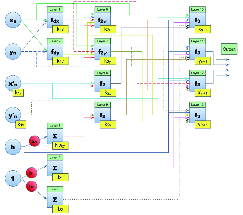
Figure 3: The constructed neural network

The neural network is constructed in such manner as to replicate the actual Runge-Kutta methodology and produce the numerical solution for the two-body problem for each step of the integration. In contrast to the actual methodology, the approximate solution at the end of each step is not used as a starting point for the next step, but instead of this, theoretical values are used as starting points for each step’s calculations.

Most of the layers do not use the standard summation function as the net input function, but a custom one, different in most of the cases. The activation function in every neuron is the identity function, described by the following equation

$$y=f(u)=u$$ (20)

Therefore, the transfer function in each case is, in essence, the net input function. Below, there is the list of the inputs and the layers of the network, their input and output connections (with any of the 6 inputs or 13 layers) and in parentheses the expression that they represent:

Input 1:

• Output connections: layers 1 ($k_{1x^{\prime}}$), 2 ($k_{1y^{\prime}}$), 6 ($k_{2x^{\prime}}$), 7 ($k_{2y^{\prime}}$), 10 ($x_{n+1}$)

• Value: $x_{n}$

Input 2:

• Output connections: layers 1 ($k_{1x^{\prime}}$), 2 ($k_{1y^{\prime}}$), 6 ($k_{2x^{\prime}}$), 7 ($k_{2y^{\prime}}$), 11 ($y_{n+1}$)

• Value: $y_{n}$

Input 3:

• Output connections: layers 8 ($k_{2x}$), 10 ($x_{n+1}$), 12 ($x^{\prime}_{n+1}$)

• Value: $x^{\prime}_{n}=k_{1x}$

Input 4:

• Output connections: layers 9 ($k_{2y}$), 11 ($y_{n+1}$), 13 ($y^{\prime}_{n+1}$)

• Value: $y^{\prime}_{n}=k_{1y}$

Input 5:

• Output connections: layers 3 ($h\,a_{21}$), 10 ($x_{n+1}$), 11 ($y_{n+1}$), 12 ($x^{\prime}_{n+1}$), 13 ($y^{\prime}_{n+1}$)

• Value: $h$

Input 6:

• Output connections: layers 4 ($b_{1}$), 5 ($b_{2}$)

• Value: $1$

Layer 1:

• Input connections: inputs 1 ($x_{n}$), 2 ($y_{n}$)

• Output connections: layers 6 ($k_{2x^{\prime}}$), 7 ($k_{2y^{\prime}}$), 12 ($x^{\prime}_{n+1}$)

• Net input function: $f_{x^{\prime}}(x_{n},y_{n})=-\frac{x_{n}}{(\sqrt{x_{n}^{2}+y_{n}^{2}})^{3}}$

• Output value: $k_{1x^{\prime}}$

Layer 2:

• Input connections: inputs 1 ($x_{n}$), 2 ($y_{n}$)

• Output connections: layers 6 ($k_{2x^{\prime}}$), 7 ($k_{2y^{\prime}}$), 13 ($y^{\prime}_{n+1}$)

• Net input function: $f_{y^{\prime}}(x_{n},y_{n})=-\frac{y_{n}}{(\sqrt{x_{n}^{2}+y_{n}^{2}})^{3}}$

• Output value: $k_{1y^{\prime}}$

Layer 3:

• Input connections: input 5 ($h$)

• Output connections: layers 6 ($k_{2x^{\prime}}$), 7 ($k_{2y^{\prime}}$), 8 ($k_{2x}$), 9 ($k_{2y}$)

• Net input function: $\sum$

• Output value: $h\,a_{21}$

Layer 4:

• Input connections: input 6 ($1$)

• Output connections: layers 10 ($x_{n+1}$), 11 ($y_{n+1}$), 12 ($x^{\prime}_{n+1}$), 13 ($y^{\prime}_{n+1}$)

• Net input function: $\sum$

• Output value: $b_{1}$

Layer 5:

• Input connections: input 6 ($1$)

• Output connections: layers 10 ($x_{n+1}$), 11 ($y_{n+1}$), 12 ($x^{\prime}_{n+1}$), 13 ($y^{\prime}_{n+1}$)

• Net input function: $\sum$

• Output value: $b_{2}$

Layer 6:

• Input connections: inputs 1 ($x_{n}$), 2 ($y_{n}$), layers 1 ($k_{1x^{\prime}}$), 2 ($k_{1y^{\prime}}$), 3 ($h\,a_{21}$)

• Output connections: layer 12 ($x^{\prime}_{n+1}$)

• Net input function: $f_{2x^{\prime}}=f_{x^{\prime}}(x_{n}+h\,a_{21}\,k_{1x^{\prime}},\,y_{n}+h\,a_{21}\,k_{1y^{\prime}})$

• Output value: $k_{2x^{\prime}}$

Layer 7:

• Input connections: inputs 1 ($x_{n}$), 2 ($y_{n}$), layers 1 ($k_{1x^{\prime}}$), 2 ($k_{1y^{\prime}}$), 3 ($h\,a_{21}$)

• Output connections: layer 13 ($y^{\prime}_{n+1}$)

• Net input function: $f_{2y^{\prime}}=f_{y^{\prime}}(x_{n}+h\,a_{21}\,k_{1x^{\prime}},\,y_{n}+h\,a_{21}\,k_{1y^{\prime}})$

• Output value: $k_{2y^{\prime}}$

Layer 8:

• Input connections: input 3 ($x^{\prime}_{n}=k_{1x}$), layer 3 ($h\,a_{21}$)

• Output connections: layer 10 ($x_{n+1}$)

• Net input function: $f_{2}=x^{\prime}_{n}+h\,a_{21}\,k_{1x}=x^{\prime}_{n}\cdot(1+h\,a_{21})$

• Output value: $k_{2x}$

Layer 9:

• Input connections: input 4 ($y^{\prime}_{n}=k_{1y}$), layer 3 ($h\,a_{21}$)

• Output connections: layer 11 ($y_{n+1}$)

• Net input function: $f_{2}=y^{\prime}_{n}+h\,a_{21}\,k_{1y}=y^{\prime}_{n}\cdot(1+h\,a_{21})$

• Output value: $k_{2y}$

Layer 10:

• Input connections: inputs 1 ($x_{n}$), 3 ($x^{\prime}_{n}=k_{1x}$), 5 ($h$), layers 4 ($b_{1}$), 5 ($b_{2}$), 8 ($k_{2x}$)

• Output connections: network output

• Net input function: $f_{3}=x_{n}+h\cdot(b_{1}\,k_{1x}+b_{2}\,k_{2x})$

• Output value: $x_{n+1}$

Layer 11:

• Input connections: inputs 2 ($y_{n}$), 4 ($y^{\prime}_{n}=k_{1y}$), 5 ($h$), layers 4 ($b_{1}$), 5 ($b_{2}$), 9 ($k_{2y}$)

• Output connections: network output

• Net input function: $f_{3}=y_{n}+h\cdot(b_{1}\,k_{1y}+b_{2}\,k_{2y})$

• Output value: $y_{n+1}$

Layer 12:

• Input connections: inputs 3 ($x^{\prime}_{n}=k_{1x}$), 5 ($h$), layers 1 ($k_{1x^{\prime}}$), 4 ($b_{1}$), 5 ($b_{2}$), 6 ($k_{2x^{\prime}}$)

• Output connections: network output

• Net input function: $f_{3}=x^{\prime}_{n}+h\cdot(b_{1}\,k_{1x^{\prime}}+b_{2}\,k_{2x^{\prime}})$

• Output value: $x^{\prime}_{n+1}$

Layer 13:

• Input connections: inputs 4 ($y^{\prime}_{n}=k_{1y}$), 5 ($h$), layers 2 ($k_{1y^{\prime}}$), 4 ($b_{1}$), 5 ($b_{2}$), 7 ($k_{2y^{\prime}}$)

• Output connections: network output

• Net input function: $f_{3}=y^{\prime}_{n}+h\cdot(b_{1}\,k_{1y^{\prime}}+b_{2}\,k_{2y^{\prime}})$

• Output value: $y^{\prime}_{n+1}$

5 Method derivation

The derivation of the coefficients for the RK method described in (2), includes certain subroutines:

• Data generation

• Neural network training

• Conversion to fraction

During the data generation phase, we generate the input and target data that are going to be used to train the neural network. We have used various integration intervals $[t_{s},t_{e}]$, from $[0,2\pi]$ up to $[0,200\pi]$ and various steplengths, from $h=\frac{\pi}{4}$ down to $\frac{\pi}{512}$. As we mentioned before, the input and the target data are described by the equations (18) and (19) respectively. Therefore, after the data generation, we obtain an input matrix of size $6\times N$ and a target matrix of size $4\times N$. Where $N$ is the number of steps and the following equation holds

$$N=\frac{t_{e}-t_{s}}{h}$$ (21)

During the training phase, we use the generated data to train the neural network. The method used to conduct the training is a variation of the typical backpropagation method, called Gradient Descent with Momentum and Adaptive Learning Rate Backpropagation or GDX. The back-propagation algorithm and its numerous variants constitute the most popular learning technique for feedforward neural networks haykin . However, a shortcoming of the original back-propagation algorithm is that it can be easily trapped in local minima. In order to deal with this disadvantage, the addition of a momentum term has been proposed. GDX includes the momentum term in order to be able to escape from local minima, but also has been found to present faster convergence and lower training times compared to other competing methods yu .

Instead of a standard error estimation function, we use a custom one for this purpose, which is shown below

$$||{\bf Output}-{\bf Target}||_{\infty}+|b_{1}+b_{2}-1|+|a_{21}\,b_{2}-\frac{1}{2}|$$ (22)

The error to be minimized is the maximum absolute difference between the output and the target data, plus some added expressions to satisfy the algebraic conditions. The terms $|b_{1}+b_{2}-1|$ and $|a_{21}\,b_{2}-\frac{1}{2}|$ are used to satisfy the conditions (5) and (6) respectively. The coefficient $a_{21}$ is used interchangeably with $c_{2}$, due to (7).

As a result of the training phase, the obtained coefficients $a_{21}$, $b_{1}$ and $b_{2}$ satisfy the conditions to a certain degree of accuracy. Additionally, the Runge-Kutta method constructed with the generated coefficients can produce an output, sufficiently close to the target data.

During the last phase, the coefficient $a_{21}$ is converted into a fraction to simplify the method, with an insignificant loss of accuracy. The rest of the coefficients are calculated with the use of the fractional $a_{21}$, in order for the algebraic and consistency conditions, (5), (6) and (7) respectively, to be satisfied. The coefficients of the new method are presented in Table 1.

For the current implementation, the number of maximum iterations was set at 10000. That value was selected empirically, as the neural network provided a solution after approximately 5000 iterations and effectively completed the training, as it could not improve on the performance any further.

6 Results

The best method was provided by using the integration interval $[0,2\pi]$ and the steplength $h=\frac{\pi}{128}$. Training with other integration intervals and steplengths have returned similar results. $2\pi$ represents a full oscillation for the two-body problem, which in part explains why training over wider intervals does not yield better results. Apart from the new method, the training has also generated some well known classical methods, some of which are given later in this section.

We compare the new method with three classical two-stage explicit Runge-Kutta methods. The corresponding Butcher tableaus of all methods are shown in Tables 1-4.

$\frac{11}{26}$	$\frac{11}{26}$
	$-\frac{2}{11}$	$\frac{13}{11}$

Table 1: New method

$1$	$1$
	$\frac{1}{2}$	$\frac{1}{2}$

Table 2: Heun’s method

$\frac{1}{2}$	$\frac{1}{2}$
	$0$	$1$

Table 3: Midpoint method

$\frac{2}{3}$	$\frac{2}{3}$
	$\frac{1}{4}$	$\frac{3}{4}$

Table 4: Third classical method

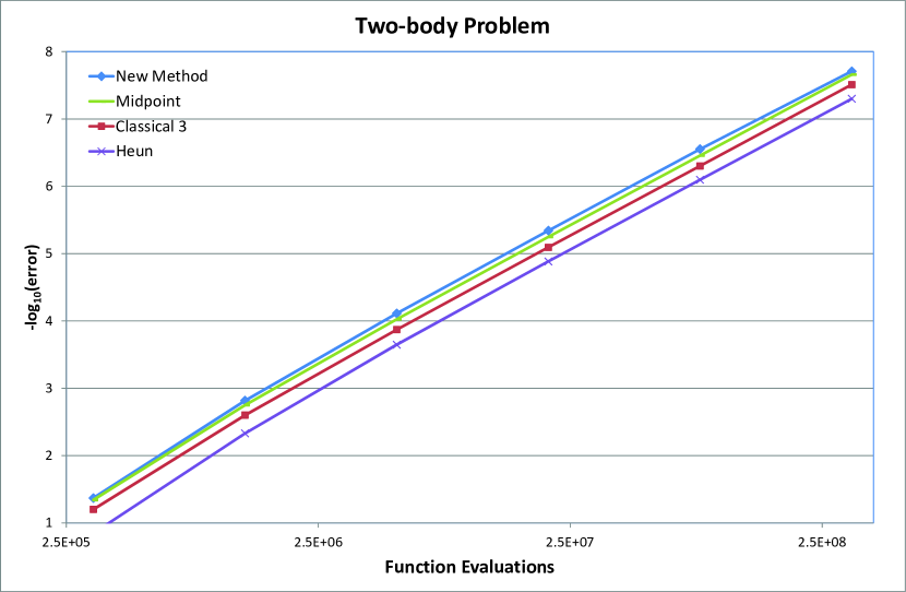
Figure 4: Efficiency of the compared methods for the integration of the two-body problem

A comparison between the classical methods and the new method is presented in figure 4, which regards the numerical integration of the two-body problem over the interval $[0,1000]$. The vertical axis represents the accuracy as expressed by $-log_{10}$(maximum absolute error), while the horizontal axis represents the total number of function evaluations that are required for the computation. The latter is provided by the formula $F.E.=s\cdot N$, where $s=2$ and stands for the number of stages of the RK method and $N$ is the number of total steps. We can see that the new method is more efficient among all methods compared.

7 Conclusions

We have constructed an artificial neural network that can generate the optimal coefficients of an explicit two-stage Runge-Kutta method. The network is specifically designed to apply to the needs of the two-body problem, and therefore the resulting method is specialized in solving that problem. Following the implementation of the network, the latter is trained to obtain the optimal values for the coefficients of the method. The comparison has shown that the new method developed in this work is more efficient than other well known methods and thus proved the capability of the constructed neural network to create new efficient numerical algorithms.

References

- (1) Cybenko G (1989) Approximations by superpositions of sigmoidal functions. Mathematics of Control, Signals, and Systems 2:303–314
- (2) Hornik K (1991) Approximation Capabilities of Multilayer Feedforward Networks. Neural Networks 4:251–257
- (3) Dissanayake MWMG, Phan-Thien N (1994) Neural-network-based approximations for solving partial differential equations. Communications in Numerical Methods in Engineering 10:195–201
- (4) Meade AJ Jr, Fernandez AA (1994) The numerical solution of linear ordinary differential equations by feedforward neural networks. Mathematical and Computer Modelling 19:1–25
- (5) Meade AJ Jr, Fernandez AA (1994) Solution of nonlinear ordinary differential equations by feedforward neural networks. Mathematical and Computer Modelling 20:19–44
- (6) Puffer F, Tetzlaff R, Wolf D (1995) Learning algorithm for cellular neural networks (CNN) solving nonlinear partial differential equations. Conference Proceedings of the International Symposium on Signals, Systems and Electronics:501–504
- (7) Lagaris IE, Likas A, Fotiadis DI (1998) Artificial neural networks for solving ordinary and partial differential equations. IEEE Transactions on Neural Networks 9:987–1000
- (8) He S, Reif K, Unbehauen R S (2000) Multilayer neural networks for solving a class of partial differential equations. Neural Networks 13:385–396
- (9) Jianyu L, Siwei L, Yingjian Q, Yaping H (2002) Numerical solution of differential equations by radial basis function neural networks. Proceedings of the International Joint Conference on Neural Networks 1:773–777
- (10) Alexandridis A, Chondrodima E, Sarimveis H (2013) Radial Basis Function Network Training Using a Nonsymmetric Partition of the Input Space and Particle Swarm Optimization. IEEE Transactions on Neural Networks and Learning Systems 24:219–230
- (11) Ramuhalli P, Udpa L, Udpa SS (2005) Finite-element neural networks for solving differential equations. IEEE Transactions on Neural Networks 16:1381–1392
- (12) Tsoulos IG, Gavrilis D, Glavas E (2009) Solving differential equations with constructed neural networks. Neurocomputing 72(10-12):2385–2391
- (13) Tsitouras C (2002) Neural Networks with multidimensional transfer functions. IEEE Transactions on Neural Networks 13:222–228
- (14) Butcher JC (2003) Numerical methods for ordinary differential equations. Wiley, New York
- (15) Haykin S (1999) Neural Networks: A Comprehensive Foundation. Prentice Hall, Englewood Cliffs, New Jersey
- (16) Widrow B, Hoff ME (1960) Adaptive switching circuits. IRE WESCON Convention Record 4:96–104
- (17) Yu CC, Liu BD (2002) A back-propagation algorithm with adaptive learning rate and momentum coefficient. Proceedings of the 2002 International Joint Conference on Neural Networks 2:1218–1223