Electron fractionalization and unconventional order parameters of the $t$-$J$ model

Abstract

In the $t$-$J$ model, the electron fractionalization is unique due to the non-perturbative phase string effect. We formulated a lattice field theory taking this effect into full account. Basing on this field theory, we introduced a pair of Wilson loops which constitute a complete set of order parameters determining the phase diagram in the underdoped regime. We also established a general composition rule for electric transport expressing the electric conductivity in terms of the spinon and the holon conductivities. The general theory is applied to studies of the quantum phase diagram. We found that the antiferromagnetic and the superconducting phases are dual: in the former, holons are confined while spinons are deconfined, and vice versa in the latter. These two phases are separated by a novel phase, the so-called Bose-insulating phase, where both holons and spinons are deconfined and the system is electrically insulating.

I Introduction

One of the canonical notions in the theory of thermal phase transition is the Landau-Ginzburg-Wilson (LGW) symmetry-breaking paradigm. For a second order phase transition, one utilizes a few “order parameters” to characterize different symmetries of the phases and thus a critical theory is in terms of fluctuations of these order parameters, which drive the system towards a critical point. In the past few years, whether the LGW paradigm may be extended to quantum phase transitions has become one of the most fascinating topics in studies of strongly correlated electronic materials. In fact, there has been substantial investigations (e.g., Refs. Fisher04 ; Fisher04a ; Balents05 ; Senthil07 ) showing that the conventional LGW paradigm fails to describe diverse quantum phase transitions. In particular, a microscopic mechanism that violates the LGW paradigm is the so-called “fractionalization”, discovered, say, in the study of two-dimensional quantum magnets Fisher04 . It suggests a very general scenario of quantum phase transitions that has been currently under intensive experimental and theoretical investigations. Basically, a quantum particle may be effectively fractionalized into a few degrees of freedom interacting via emergent gauge field, and some fractionalized degrees of freedom appear at the critical point but not in the stable phases at each side of the critical point.

Thus, as correlated electronic systems are concerned, a fundamental issue is: how does the electron fractionalization, where electrons are effectively fractionalized into the spin and the charge degrees of freedom at short scales, lead to various phases and the phase transitions between them? In one dimension, it has been well established that the spin-charge separation results in the Tomonaga-Luttinger liquid. In contrast, less has been known about the interplay between the electron fractionalization and quantum phase transitions, notably in the two-dimensional doped Mott insulator Anderson87 which is widely accepted to be the prototype of high temperature superconductors Lee06 ; Fisher00 ; Sachdev03 . Notwithstanding, experimental and theoretical analysis indicating the electron fractionalization to be at the root of low-dimensional strongly correlated electronic systems has been well documented. In fact, there exist two classes of experiments on cuprate materials, namely the large Nernst effect in thermoelectric transport measurements Ong04 and the periodic modulations of electronic density of states in scanning tunneling microscopy studies Takagi04 . It has been pointed out Balents05 that a LGW-type theory trying to reconcile these two phenomena cannot be, at least, extended to zero temperature. Instead, substantial theoretical analysis shows that the electron fractionalization necessarily leads to new quantum phases Lee06 . This opinion has been reiterated very recently by Zaanen and Overbosch Zaanen09 , who pointed out that the drastic change in the nature of quantum statistics upon doping – a direct manifestation of the electron fractionalization – may be the key to understanding physics of the pseudogap phase. Central to these studies are a number of fundamental issues. The most prominent ones include: What kind of quantum statistics do the emergent degrees of freedom obey? How do they interact with each other? How does the electron fractionalization turn an antiferromagnet into a superconductor upon doping? What does the phase diagram look like?

While to investigate these issues for general doped Mott insulators proves to be highly challenging, in this work, we switch to a limiting case where the on-site Coulomb repulsion is strong enough, namely the $t$-$J$ model (on a bipartite lattice), and will present an analytical study of the above problems. Our starting point is an exact non-perturbative result for this model, the so-called phase string effect discovered some time ago Weng97 . Specifically, the motion of a hole may leave a trace on the lattice plane upon colliding with spins. The phase string effect means that such two nearby propagating paths of the hole, though possessing (almost) identical amplitudes, may substantially differ in the phases by $\pi$ (namely in the overall sign). Such a sign structure accounts for the parity of the number of hole–spin collisions and is thereby intrinsic to individual paths. Most importantly, with this effect being taken into full account, it turns out (to be detailed in this work) that an electron is uniquely, rather than arbitrarily, fractionalized into two bosonic constituents namely the holon and the spinon, satisfying a mutual statistical interaction. Basing on this exact result, in this work, we will study–at a full microscopic level–how a phase diagram flows out of electron fractionalization.

The main results of this work were briefly reported in our earlier publication Ye11 . The present paper is devoted to reporting the technical details and the remaining is organized as follows. For the self-contained purposes we will briefly review the phase string effect in Sec. II and, particularly, introduce the emergent mutual statistical interaction. In Sec. III, we will formulate a general lattice field theory basing on the phase string effect and introduce a pair of unconventional order parameters. Using this general theory, we will present a general result for electric transport in Sec. IV. In particular, we will prove a composition rule that expresses the electric conductivity in terms of holon and spinon conductivities. Armed with the pair of unconventional order parameters and the composition rule, we will explore the quantum phase diagram in Sec. V. (Throughout this paper, we shall focus on the underdoped regime.) Finally, we will conclude in Sec. VI. Some of the technical details are regelated to Appendices A-C.

II Phase string effect: a short review

For the self-contained purpose we shall start from a brief exposition of the exact phase string effect Weng07 for the $t$-$J$ model ($t,J>0$)

$$H=-t\sum_{\langle i,j\rangle}\sum_{\sigma}\,\left({c}_{i\sigma}^{\dagger}{c}_{j\sigma}+{\rm h.c.}\right)+J\sum_{\langle i,j\rangle}\left(S_{i}\cdot{S}_{j}-\frac{{n}_{i}{n}_{j}}{4}\right)\equiv H_{t}+H_{J}$$ (1)

on a square lattice, where ${\rm h.c.}$ stands for the hermitian conjugate. In this Section, in particular, we will discuss the physical picture of the mutual statistical interaction between holons and spinons, as well as its mathematical origin. In Eq. (1), $c_{i\sigma}^{\dagger}$ ($c_{i\sigma}$) is the (fermionic) electron creation (annihilation) operator on site $i$ with the spin polarization $\sigma=\downarrow,\uparrow$ , $n_{i}\equiv\sum_{\sigma}c_{i\sigma}^{\dagger}c_{i\sigma}$ is the occupation number operator, $S_{i}$ is the spin operator, and $\langle i,j\rangle$ stands for the link between two nearest neighbors $i$ and $j$. Note that throughout this work, we shall not distinguish notationally the difference between the operators and the numbers. The wave function is restricted on the Hilbert space such that no sites are occupied by more than one electron–the no-double-occupancy constraint. Eq. (1) together with the no-double-occupancy constraint serve as the exact starting point of the present work.

II.1 Bosonization: phase-string representation

In Eq. (1) the first ($H_{t}$) and the second ($H_{J}$) term describe the charge hopping and the spin-flip process, respectively. The latter is reduced into the Heisenberg model in the undoped (half-filling) case where ${n}_{i}=1$ . For this case, long time ago Marshall showed that the matrix element of the superexchange Hamiltonian must satisfy a sign rule Marshall55 . That is, there exists a complete set of spin bases $\{|\phi\rangle\}$ such that given arbitrary spin configurations $\phi$ and $\phi^{\prime}$ ,

$$\langle\phi^{\prime}|H_{J}|\phi\rangle\leq 0\,.$$ (2)

For doped antiferromagnets the Marshall sign rule (2) may be trivially realized within the Schwinger-boson (${b}_{i\sigma}^{\dagger},{b}_{i\sigma}$), slave-fermion (${f}_{i}^{\dagger},{f}_{i}$) formalism, provided that the spin-hole bases $\{|\phi\rangle\}$ are chosen appropriately. Under these bases the superexchange and hopping Hamiltonian are written as Weng97

$$H_{J} = -\frac{J}{2}\sum_{\langle i,j\rangle}\sum_{\sigma\sigma^{\prime}}\,{b}_{i\sigma}^{\dagger}{b}_{j-\sigma}^{\dagger}{b}_{j-\sigma^{\prime}}{b}_{i\sigma^{\prime}}\,,$$ (3)

$$H_{t} = -t\sum_{\langle i,j\rangle}\sum_{\sigma}\,\sigma{f}_{i}^{\dagger}{f}_{j}{b}_{j\sigma}^{\dagger}{b}_{i\sigma}+{\rm h.c.}\,.$$ (4)

Note that the sign of $H_{J}$ is now negative. Here the “holon” creation operator ${f}_{i}^{\dagger}$ and the “spinon” annihilation operator ${b}_{i\sigma}$ commute with each other, and satisfy the no-double-occupancy constraint:

$${f}_{i}^{\dagger}{f}_{i}+\sum_{\sigma}{b}_{i\sigma}^{\dagger}{b}_{i\sigma}=1\,.$$ (5)

The sign structure in $H_{t}$ (arising from hole-spin exchange) results in peculiar properties. Technically, it prohibits a perturbative expansion of the resolvent: $(E-H_{J}-H_{t})^{-1}$ even in $t/J\ll 1$. Physically, it accounts for the fact Weng97 ; Weng07 that the holon, upon hopping to some site occupied instantly by a $\uparrow$ ($\downarrow$)-spin, acquires a sign $+1$ ($-1$). (As such, the Marshall sign rule is incompatible with the hopping process.) Therefore, two holon paths close to each other, though having (almost) identical amplitudes, may differ in the sign, because the parity of the number of hole–$\downarrow$-spin collisions of each paths may be different. This is the so-called phase string effect and possesses non-perturbative nature.

Before further proceeding, it is necessary to take this non-perturbative phase-string effect into full account. Such a task was fulfilled in Ref. Weng97 by introducing the so-called phase string transformation:

$$|\psi\rangle\rightarrow e^{i{\Theta}}\,|\psi\rangle\,,\qquad{O}\rightarrow e^{i{\Theta}}{O}e^{-i{\Theta}}\,,$$ (6)

which exactly “gauges away” the phase string arising from the holon hopping. In Eq. (6) the phase string operator ${\Theta}$ is defined as

$${\Theta}\equiv-\sum_{i,j}\,{n}_{i}^{h}\,\theta_{ij}\,{n}^{s}_{j\downarrow}\,,\qquad\theta_{ij}\equiv{\rm Im}\ln(z_{i}-z_{j})\in[-\pi,+\pi)\,,$$ (7)

where ${n}^{h}_{i}$ and ${n}^{s}_{i\sigma}$ are the holon and the spinon occupation number operator, respectively. Note that the two-dimensional lattice spans a complex plane and $z$ is the position of the spinon (holon) in this complex plane. Moreover, the no-double-occupancy constraint implies that the summation excludes automatically the term with $i=j$ .

Let us now apply the phase-string transformation (6) to Eqs. (3) and (4). Introduce the bosonic operator ${h}_{i}^{\dagger}\,,{h}_{i}$ :

$${h}_{i}^{\dagger}\equiv{f}_{i}^{\dagger}\,\exp\left(-i\sum_{l\neq i}\theta_{il}{n}_{l}^{h}\right)\,,\qquad{h}_{i}\equiv\exp\left(i\sum_{l\neq i}\theta_{il}{n}_{l}^{h}\right)\,{f}_{i}$$ (8)

which preserves the no-double-occupancy constraint:

$${h}_{i}^{\dagger}{h}_{i}+\sum_{\sigma}{b}_{i\sigma}^{\dagger}{b}_{i\sigma}=1\,.$$ (9)

Then, $H_{J,t}$ are transformed to

$$H_{J} \rightarrow -\frac{J}{2}\sum_{\langle i,j\rangle}\sum_{\sigma\sigma^{\prime}}\,e^{i\sigma A_{ij}^{h}}\,b_{i\sigma}^{\dagger}b_{j-\sigma}^{\dagger}e^{i\sigma^{\prime}A_{ji}^{h}}\,b_{j-\sigma^{\prime}}b_{i\sigma^{\prime}}\,,$$ (10)

$$H_{t} \rightarrow -t\sum_{\langle i,j\rangle}\sum_{\sigma}\,e^{iA_{ij}^{s}}\,h_{i}^{\dagger}h_{j}e^{i\sigma A_{ji}^{h}}\,b_{j\sigma}^{\dagger}b_{i\sigma}+{\rm h.c.}\,,$$ (11)

where the gauge fields $A_{ij}^{s,h}$ given by

$$A_{ij}^{s} \equiv \frac{1}{2}\sum_{l\neq i,j}\,\left(\theta_{il}-\theta_{jl}\right)\left(n^{s}_{l\uparrow}-n^{s}_{l\downarrow}\right)\,\,{\rm mod}\,2\pi\,,$$ (12)

$$A_{ij}^{h} \equiv \frac{1}{2}\sum_{l\neq i,j}\,\left(\theta_{il}-\theta_{jl}\right)n^{h}_{l}\,\,{\rm mod}\,2\pi$$ (13)

are angular variables. Eqs. (10)-(13) constitute the exact bosonization of the original $t$-$J$ model (1) subject to the no-double-occupancy constraint.

II.2 Mutual statistical interaction and compact gauge symmetry

Consider now an arbitrary loop $C$ on the lattice plane. Eqs. (12) and (13) give unit

$$\sum_{\langle i,j\rangle\in C}\,A_{ij}^{s} = \pi\sum_{l\in S_{C}}\,\left(b^{\dagger}_{l\uparrow}b_{l\uparrow}-b^{\dagger}_{l\downarrow}b_{l\downarrow}\right)\,\,{\rm mod}\,2\pi\,,$$ (14)

$$\sum_{\langle i,j\rangle\in C}\,A_{ij}^{h} = \pi\sum_{l\in S_{C}}\,h^{\dagger}_{l}h_{l}\,\,{\rm mod}\,2\pi\,,$$ (15)

where on the left hand side the sum runs over all the links on $C$ , while on the right hand side the sum runs over all the sites inside $C$ . Eqs. (14) and (15) show that the holon (spinon) carries a $\pi$-flux and couples to the motion of spinons (holons) via the gauge field $A_{ij}^{h}$ ($A_{ij}^{s}$). We see that the phase string effect effectively “fractionalizes” an electron into two topological objects – the spinon and the holon – and the spin and charge degrees of freedom obeys a mutual statistical interaction. This kind of interaction was also found in different contexts Xu09 ; Galitskii05 ; DST06 .

It is of conceptual importance that the present theory differs from the earlier one KQW05 in the emergence of the local compact (instead of non-compact) $U(1)\otimes U(1)$ gauge symmetry, where the two $U(1)$ gauge degrees of freedom couple to the holon and the spinon, respectively. Indeed, Eqs. (10), (11), (14) and (15) are invariant under the following gauge transformation (All the quantities here may depend on the imaginary time $\tau$.):

$$\begin{array}[]{c}A_{ij}^{s,h}\rightarrow A_{ij}^{s,h}+\theta_{i}^{s,h}-\theta_{j}^{s,h}\,,\\ b_{i\sigma}^{\dagger}\rightarrow b_{i\sigma}^{\dagger}\,e^{-i\sigma\theta_{i}^{h}}\,,\qquad b_{i\sigma}\rightarrow b_{i\sigma}\,e^{i\sigma\theta_{i}^{h}}\,,\qquad h_{i}^{\dagger}\rightarrow h_{i}^{\dagger}\,e^{-i\theta_{i}^{s}}\,,\qquad b_{i\sigma}\rightarrow b_{i\sigma}\,e^{i\theta_{i}^{s}}\,,\end{array}$$ (18)

and are apparently invariant upon shifting $A^{s,h}_{ij}$ by $2\pi$ . Importantly, due to the single-valued nature the following mapping

$$\theta^{s,h}:{\cal C}^{s,h}\mapsto U(1)$$ (19)

from an arbitrary loop ${\cal C}^{s,h}$ in spacetime lattice to the gauge group $U(1)$ has the homotopy group $\mathbb{Z}$.

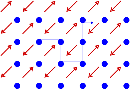
Figure 1: Dual lattice regularization: the lattice (red arrow) where spinons reside is separated from the lattice (blue circle) supporting the holon motion (presented by the path).

III Lattice field theory and unconventional order parameters

Our theory has so far been exact. In the remaining of this paper we will study the mean field approximation of Eqs. (10) and (11), read

$$H_{s} = -J_{s}\sum_{\langle ij\rangle}\sum_{\sigma}\,e^{i\sigma\,A_{ij}^{h}}\,b_{i\sigma}^{\dagger}b_{j-\sigma}^{\dagger}+{\rm h.c.}\,,$$ (20)

$$H_{h} = -t_{h}\sum_{\langle ij\rangle}\,e^{iA_{ij}^{s}}\,h_{i}^{\dagger}h_{j}+{\rm h.c.}\,.$$ (21)

The “minimal” Hamiltonian $H_{h}+H_{s}$ and Eqs. (12) and (13) constitute the so-called phase string model. It is important that this model preserves the compact $U(1)\otimes U(1)$ gauge symmetry.

To further proceed we introduce the dual lattice regularization KQW05 . Basically, the spinon and the holon reside in their own square sublattice (Fig. 1). The advantage of this ultraviolet regularization is as follows: as the constraints (14) and (15) are concerned, in the right-hand side of these two equations, the holon (spinon) does not appear on the loop $C$ (We stress, however, that this is merely for the purpose of technical simplicity and violating this condition does not lead to changes of the results reported in this paper.). The spinon coordinate system is denoted as $x\equiv(i_{1},i_{2},i_{0})$, where the first two components refer to the lattice point in the $x$-$y$ plane and the last to the (discrete) imaginary time. We set the lattice constant to unity. The holon coordinate system is denoted as $x\equiv(I_{1},I_{2},I_{0})$, with the origin as $(-\frac{1}{2},-\frac{1}{2},0)$ in the holon coordinate system. The gauge field $A^{h}_{x+{\hat{\mu}}x}\equiv A^{h}_{\mu}(x)$ is defined on the spinon lattice, while $A^{s}_{xx-{\hat{\mu}}}\equiv A^{s}_{\mu}(x)$ [as well as the external electromagnetic field $A^{e}_{xx-{\hat{\mu}}}\equiv A^{e}_{\mu}(x)$] is defined on the holon lattice. Here, we denote the unit vector in the $\mu$ direction as $\hat{\mu}$. Finally, wherever a lattice function $f(i,I)$ is involved the relation $(I_{1},I_{2},I_{0})=(i_{1}+\frac{1}{2},i_{2}+\frac{1}{2},i_{0})$ is implied for the arguments, and throughout this paper, the Greek indices $\mu,\nu,\lambda$ run over both the spatial and the temporal components, while $\alpha,\beta$ only over the spatial component.

Consider the partition function ${\cal Z}\equiv{\rm Tr}\exp(-\beta{\cal H})$ . Here, $\beta$ is the inverse temperature and the Hamiltonian is

$${\cal H}\equiv-t_{h}\sum_{I\alpha}\left(e^{iA^{s}_{\alpha}}h^{\dagger}_{I}h_{I-{\hat{\alpha}}}+{\rm h.c.}\right)-J_{s}\sum_{i\alpha\sigma}\left(e^{i\sigma A^{h}_{{\alpha}}}b^{\dagger}_{i+{\hat{\alpha}}\sigma}b^{\dagger}_{i-\sigma}+{\rm h.c.}\right)$$ (22)

under the dual lattice regularization. Then, it is a canonical procedure to divide $\beta$ into ${\cal N}$ pieces, and for each imaginary time slice we insert the unit resolution. Upon sending ${\cal N}$ to infinity we expect to obtain an expression of ${\cal Z}$ in terms of the path integral of the configuration of the gauge fields $A_{\alpha}^{s,h}$ and the matter fields $h,b$ (as well as their complex conjugates $h^{\dagger},b^{\dagger}$). All the fields are in turn imaginary time-dependent (which, however, is suppressed to simplify notations wherever no confusions arise). We now facilitate this general program by two steps.

Step I. We absorb formally the constraints enforcing on the gauge fields by the compactness into the measure, obtaining an expression for the partition function which is determined by an auxiliary Lagrangian ${\cal L}$ ;

Step II. We work out the constraints explicitly, prompting ${\cal L}$ to a new Lagrangian $\mathscr{L}$.

III.1 Mutual Chern-Simons term

We begin with Step I. To this end we note that for each imaginary time slice $\tau=j\beta/{\cal N}\,,j=1,2,\cdots,{\cal N}$ , the topological constraints (14) and (15) imposed on each plaquette give

$$\begin{array}[]{c}\mathscr{F}_{A^{s}}\equiv\epsilon^{0\alpha\beta}{d}_{\alpha}A^{s}_{\beta}-\pi\left(b^{\dagger}_{i\uparrow}b_{i\uparrow}-b^{\dagger}_{i\downarrow}b_{i\downarrow}\right)=0\,,\\ \mathscr{F}_{A^{h}}\equiv\epsilon^{0\alpha\beta}d_{\alpha}A^{h}_{\beta}-\pi h^{\dagger}_{I}h_{I}=0\,,\end{array}$$ (25)

where we define the (spacetime) lattice derivative as $d_{\mu}f(x)=f(x+{\hat{\mu}})-f(x)$ for the spinon lattice and as $d_{\mu}f(x)=f(x)-f(x-{\hat{\mu}})$ for the holon lattice, with $f(x)$ an arbitrary lattice function. Taking this into account we find

$${{\cal Z}}=\int D_{A}[A_{\alpha}^{s},A^{h}_{\alpha}]D[h^{\dagger},h,b^{\dagger},b]\delta(\mathscr{F}_{A^{s}})\delta(\mathscr{F}_{A^{h}})e^{-\sum_{x}{\cal L}_{\rm M}|_{A_{0}^{s}=A_{0}^{h}=0}}\,,$$ (26)

with the Lagrangian

$${\cal L}_{\rm M} = h_{I}^{\dagger}(d_{0}-iA_{0}^{s}+\lambda^{h})h_{I}+t_{h}\sum_{\alpha}\left(e^{iA^{s}_{\alpha}}h^{\dagger}_{I}h_{I-{\hat{\alpha}}}+{\rm c.c.}\right)$$ (27)

$$+\sum_{\sigma}b^{\dagger}_{i\sigma}(d_{0}-i\sigma A_{0}^{h}+\lambda^{s})b_{i\sigma}+J_{s}\sum_{\alpha\sigma}\left(e^{i\sigma A^{h}_{{\alpha}}}b^{\dagger}_{i+{\hat{\alpha}}\sigma}b^{\dagger}_{i-\sigma}+{\rm c.c.}\right)\,.$$

Here ${\rm c.c.}$ stands for the complex conjugate, and the subscript “$A$” in the measure $D_{A}$ for that as the integral over the gauge fields are concerned, the constraints enforced by the compactness (which will be work out explicitly in the next subsection) are implied. The parameters $\lambda^{s,h}$ are to be determined below. The constraint $\delta(\mathscr{F}_{A^{s}})\,\delta(\mathscr{F}_{A^{h}})$ may be released by introducing two real number valued fields $A_{0}^{s}(x)\,,A_{0}^{h}(x)\in\mathbb{R}$ . As a result we obtain

$${{\cal Z}}=\int D_{A}[A_{\alpha}^{s},A_{\alpha}^{h}]D_{A}[A_{0}^{s},A_{0}^{h}]D[h^{\dagger},h,b^{\dagger},b]\exp\left\{-\sum_{x}\left({\cal L}_{\rm M}+{\cal L}^{\prime}_{\rm CS}\right)\right\},$$ (28)

where the mutual Chern-Simons term is

$${\cal L}^{\prime}_{\rm CS}=\frac{i}{\pi}\left(A_{0}^{s}\epsilon^{0\alpha\beta}d_{\alpha}A^{h}_{\beta}+A_{0}^{h}\,\epsilon^{0\alpha\beta}{d}_{\alpha}A^{s}_{\beta}\right)\,.$$ (29)

The exponent in Eq. (28) is invariant merely under the imaginary time-independent transverse gauge transformation:

$$A^{h}_{\alpha}\rightarrow A^{h}_{\alpha}+d_{\alpha}\theta^{h}\,,\qquad b_{\sigma}\rightarrow b_{\sigma}e^{i\sigma\theta^{h}}\,,\qquad b^{\dagger}_{\sigma}\rightarrow b^{\dagger}_{\sigma}e^{-i\sigma\theta^{h}}\,,$$

$$A^{s}_{{\alpha}}\rightarrow A^{s}_{{\alpha}}+d_{\alpha}\theta^{s}\,,\qquad h\rightarrow he^{i\theta^{s}}\,,\qquad h^{\dagger}\rightarrow h^{\dagger}e^{-i\theta^{s}}$$ (30)

with $\theta^{s,h}$ some regular lattice functions. On the physical ground we expect that ${\cal L}^{\prime}_{\rm CS}$ possesses a natural extension Altland :

$${\cal L}^{\prime}_{\rm CS}\rightarrow{\cal L}_{\rm CS}=\frac{i}{\pi}\epsilon^{\mu\nu\lambda}A_{\mu}^{s}d_{\nu}A^{h}_{\lambda}\,.$$ (31)

As such, the action: $\sum_{x}({\cal L}_{\rm M}+{\cal L}_{\rm CS})$ is invariant under the full local $U(1)\otimes U(1)$ gauge transformation (18). In Appendix A we present an alternative derivation of this Lagrangian.

Note that the elevation: ${\cal L}^{\prime}_{\rm CS}\rightarrow{\cal L}_{\rm CS}$ is merely due to the lift of gauge fixing. This is most easily seen by reversing the procedure. Suppose that we choose the Coulomb gauge, the gauge fields are then composed of purely transverse components which may be explicitly written as Altland $A_{\perp}^{s}=({d}_{y}\theta^{s},-{d}_{x}\theta^{s},\phi^{s})$ and $A_{\perp}^{h}=(d_{y}\theta^{h},-d_{x}\theta^{h},\phi^{h})$ with $\phi^{s,h}$ and $\theta^{s,h}$ some functions in the spacetime lattice. (The first two components of $A_{\perp}^{s,h}$ are the spatial components while the last one the temporal component.) Inserting this expression into $\sum_{x}{\cal L}_{\rm CS}$ we, indeed, end up with $\sum_{x}{\cal L}^{\prime}_{\rm CS}$ . One must caution that such an elevation may generally result in a normalization factor of ${\cal Z}$ accounting for the gauge degree of freedom. However, it does not lead to any physical results and we, therefore, shall ignore this factor.

To proceed further, we divide the spinon lattice into two sublattices, say A and B. The spinon field in the sublattice A is denoted in the same way as before while in the sublattice B is denoted as $({\bar{b}},{\bar{b}}^{\dagger})$. Furthermore, we introduce a four-component vector, $\Psi_{i}$ ($i\in{\rm A}$), as follow:

$$\Psi_{i}\equiv\left(\begin{array}[]{c}\psi_{i}\\ {\bar{\psi}}_{i}\\ \end{array}\right)\,,\qquad\psi_{i}\equiv\left(\begin{array}[]{c}b_{i\uparrow}\\ b_{i\downarrow}\\ \end{array}\right)\,,\qquad{\bar{\psi}}_{i}\equiv\left(\begin{array}[]{c}\frac{1}{4}({\bar{b}}^{\dagger}_{i+\hat{x}\uparrow}+{\bar{b}}^{\dagger}_{i-\hat{x}\uparrow}+{\bar{b}}^{\dagger}_{i+\hat{y}\uparrow}+{\bar{b}}^{\dagger}_{i-\hat{y}\uparrow})\\ \frac{1}{4}({\bar{b}}^{\dagger}_{i+\hat{x}\downarrow}+{\bar{b}}^{\dagger}_{i-\hat{x}\downarrow}+{\bar{b}}^{\dagger}_{i+\hat{y}\downarrow}+{\bar{b}}^{\dagger}_{i-\hat{y}\downarrow})\\ \end{array}\right)\,.$$ (38)

Assuming the spinon fields are smooth over the (spatial) scale of the lattice constant, the Lagrangian ${\cal L}_{M}$ is re-expressed as

$${\cal L}_{\rm M} = h^{\dagger}\left(\hat{D}_{0}^{s}+\lambda^{h}-t_{h}(2+\hat{D}^{s})\right)h+\Psi^{\dagger}{\cal M}\Psi\,,$$ (39)

$${\cal M} = \left(\begin{array}[]{cccc}\hat{D}_{0}^{h}+\lambda^{s}&0&0&-J_{s}(2+(\hat{D}^{h})^{*})\\ 0&(\hat{D}_{0}^{h})^{*}+\lambda^{s}&-J_{s}(2+\hat{D}^{h})&0\\ 0&-J_{s}(2+\hat{D}^{h})&-(\hat{D}_{0}^{h})^{*}+\lambda^{s}&0\\ -J_{s}(2+(\hat{D}^{h})^{*})&0&0&-\hat{D}_{0}^{h}+\lambda^{s}\end{array}\right)\,.$$ (44)

Here, $\hat{D}_{0}^{s}\equiv d_{0}-iA_{0}^{s}$ and $\hat{D}_{0}^{h}\equiv d_{0}-iA_{0}^{h}$ are covariant time derivatives. $\hat{D}^{s}\equiv\sum_{\alpha}(d_{\alpha}-iA_{\alpha}^{s})^{2}$ and $\hat{D}^{h}\equiv\sum_{\alpha}(d_{\alpha}-iA_{\alpha}^{h})^{2}$ are (covariant) discrete Laplacians. (Notice that all the fields above are non-singular and, therefore, we may perform a hydrodynamic expansion. Alluding to this, the Laplacians result.) Finally, the partition function is written as

$${{\cal Z}}=\int D_{A}[A^{s},A^{h}]D[h^{\dagger},h,\Psi^{\dagger},\Psi]\,e^{-\sum_{x}({\cal L}_{\rm M}+{\cal L}_{\rm CS})}\,.$$ (45)

III.2 Lattice field theory

So far, the construction of the field theory has been restricted on the topological trivial sector in the sense that the mapping (19) from arbitrarily given loop ${\cal C}^{s,h}$ onto $U(1)$ has zero winding number. Therefore, the field theory achieved in Step I does not carry any information regarding the compactness of the intrinsic gauge group. To fulfill Step II let us start from analyzing the mapping (19). It implies that in the spinon lattice, a loop ${\cal C}^{\prime}$ may pass through the area circulated by the loop ${\cal C}^{s}$ once (Fig. 2) such that

$$\epsilon^{\mu\nu\lambda}{d}_{\nu}{d}_{\lambda}\theta^{s}(x)=2\pi M^{s}\sum_{x^{\prime}}J_{{\cal C}^{\prime}}^{\mu}(x^{\prime}),\qquad M^{s}\in\mathbb{Z}\,.$$ (46)

Here, the link field $J_{\cal C}^{\mu}(x)$ takes the value of $+1$ ($-1$) for the link $\langle xx+{\hat{\mu}}\rangle$ ($\langle x+{\hat{\mu}}x\rangle$) on ${\cal C}$ and zero otherwise. Under the gauge transformation, the action $\sum_{x}({\cal L}_{\rm M}+{\cal L}_{\rm CS})$ is transformed to

$$\sum_{x}({\cal L}_{\rm M}+{\cal L}_{\rm CS})\rightarrow\sum_{x}({\cal L}_{\rm M}+{\cal L}_{\rm CS})+\frac{i}{\pi}\sum_{x}\epsilon^{\mu\nu\lambda}{d}_{\mu}\theta^{s}d_{\nu}A^{h}_{\lambda}=\sum_{x}({\cal L}_{\rm M}+{\cal L}_{\rm CS})-\frac{i}{\pi}\sum_{x}\epsilon^{\lambda\mu\nu}A^{h}_{\lambda}{d}_{\mu}{d}_{\nu}\theta^{s}\,,$$ (47)

where in deriving the second equality we used the integral by parts. In order for the lattice field theory to be unaffected we demand that the second term of Eq. (47) to be multiple of $2\pi$ . Taking Eq. (46) into account we obtain

$$\sum_{x}\,J_{{\cal C}^{\prime}}^{\mu}(x)\,A_{\mu}^{h}(x)=0\,{\rm mod}\,\,\pi\,.$$ (48)

Using the Stokes’ theorem, we obtain $\sum_{x}(d_{\mu}A_{\nu}^{h}-d_{\nu}A_{\mu}^{h})\Delta S_{x}^{\mu\nu}[S_{{\cal C}^{\prime}}]=0\,{\rm mod}\,\,\pi$ with $\Delta S_{x}^{\mu\nu}[S_{{\cal C}^{\prime}}]$ the unit surface element at $x$ . (Note that here no summation is implied for $\mu,\nu$ .) Since the loop ${\cal C}^{\prime}$ and thereby the surface $S_{{\cal C}^{\prime}}$ are rather general, Eq. (48) then implies

$$d_{\mu}A_{\nu}^{h}-d_{\nu}A_{\mu}^{h}=0\,{\rm mod}\,\,\pi\,.$$ (49)

That is, the Maxwell tensor of $A^{h}$ is locally quantized, with a quanta $\pi$ . Likewise, we have

$${d}_{\mu}A_{\nu}^{s}-{d}_{\nu}A_{\mu}^{s}=0\,{\rm mod}\,\,\pi\,.$$ (50)

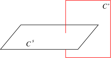
Figure 2: The loop ${\cal C}^{\prime}$ passes through the area circulated by another loop ${\cal C}^{s}$.

Eqs. (49) and (50) are the exact constraints absorbed in the measure $D_{A}[A^{s},A^{h}]$ of Eq. (45). To release such constraints we further introduce two dual integer fields $\mathscr{N}^{h}_{\mu}$ and $\mathscr{N}^{s}_{\mu}$ . In doing so we eventually obtain the path integral representation of the partition function ${\cal Z}$ , which is

$$\mathcal{Z}=\sum_{\{\mathscr{N}^{s,h}\}}\int D[A^{s},A^{h}]D[h^{\dagger},h,\Psi^{\dagger},\Psi]\,\exp\left\{-\sum_{x}\left[\mathcal{L}_{\rm M}+\mathcal{L}_{\rm CS}-2i\epsilon^{\mu\nu\lambda}\left(A^{h}_{\mu}d_{\nu}\mathscr{N}^{s}_{\lambda}+A^{s}_{\mu}{d}_{\nu}\mathscr{N}^{h}_{\lambda}\right)\right]\right\}\,.$$ (51)

III.3 Symmetries

We turn now to examine various symmetries of the action in Eq. (51). First of all, it is apparently invariant under the local $U(1)\otimes U(1)$ gauge transformation (18). Then, we absorb the integer fields $\mathscr{N}^{s,h}$ into the mutual Chern-Simons term. In doing so we reduce the Lagrangian in Eq. (51) into

$$\mathcal{L}_{\rm M}+\frac{i}{\pi}\,\epsilon^{\mu\nu\lambda}\left(A^{s}_{{\mu}}-2\pi\mathscr{N}^{s}_{\mu}\right)d_{\nu}\left(A^{h}_{{\lambda}}-2\pi\mathscr{N}^{h}_{\lambda}\right)\,,$$ (52)

where we ignore the irrelevant term multiple of $2\pi$. From this we see that the field theory is compact in the gauge degrees of freedom, because a multiple $2\pi$ shift of the gauge fields is absorbed by the integer fields. Such property is intrinsic to the discrete lattice geometry but not to the dual lattice regularization. It is also easy to see that the Lagrangian possesses both parity and time-reversal symmetry KQW05 . Under parity transformation $\mathscr{N}^{h}$ transforms as an axial vector while $\mathscr{N}^{s}$ as a polar vector. Under time-reversal operation $\mathscr{N}^{s,h}$ transforms as

$$\mathscr{N}^{s}_{0}\rightarrow\mathscr{N}^{s}_{0}\,,\,\mathscr{N}^{s}_{\alpha}\rightarrow-\mathscr{N}^{s}_{\alpha}\,;\qquad\mathscr{N}^{h}_{0}\rightarrow-\mathscr{N}^{h}_{0}\,,\,\mathscr{N}^{h}_{\alpha}\rightarrow\mathscr{N}^{h}_{\alpha}\,.$$ (53)

We further show that the Lagrangian possesses the spin rotation symmetry. Indeed, transforming $\Psi_{i}$ as

$$\Psi_{i}\rightarrow\left(\begin{array}[]{cc}e^{i\sigma_{3}\Phi_{i}^{h}/2}&0\\ 0&e^{-i\sigma_{3}\Phi_{i}^{h}/2}\\ \end{array}\right)\left(\begin{array}[]{cc}U(\theta,\phi,\chi)&0\\ 0&U(-\theta,-\phi,-\chi)\\ \end{array}\right)\left(\begin{array}[]{cc}e^{-i\sigma_{3}\Phi_{i}^{h}/2}&0\\ 0&e^{i\sigma_{3}\Phi_{i}^{h}/2}\\ \end{array}\right)\Psi_{i}\,,$$ (60)

we find that the Lagrangian is invariant. Note that the $2\times 2$ matrices above are defined on the sector introduced by the doublet due to the sublattice structure [cf. the definition of $\Psi_{i}$ in Eq. (38)], while $U$ and $\sigma_{3}=\left(\begin{array}[]{cc}1&0\\ 0&-1\\ \end{array}\right)$ are defined on the spin sector [cf. the definitions of $\psi_{i}$ , $\bar{\psi}_{i}$ in Eq. (38)]. The spin rotation is generated by the Euler angles $\theta,\phi$ and $\chi$, i.e.,

$$U(\theta,\phi,\chi)=\left(\begin{array}[]{cc}\cos\frac{\theta}{2}e^{i\phi/2}e^{i\chi/2}&\sin\frac{\theta}{2}e^{-i\phi/2}e^{i\chi/2}\\ -\sin\frac{\theta}{2}e^{i\phi/2}e^{-i\chi/2}&\cos\frac{\theta}{2}e^{-i\phi/2}e^{-i\chi/2}\\ \end{array}\right)\,.$$ (63)

Finally, the single-valueness of transformed $\Psi_{i}$ is guaranteed by the relation $d_{\mu}\Phi^{h}=2A^{h}_{\mu}$ and Eq. (49). The present theory shows that the spin rotation symmetry is protected against high-energy ferromagnetic fluctuations, while the earlier theory KQW05 proves the existence of this symmetry only for the low-energy sector.

To proceed further, we wish to soften the hard-core boson condition, i.e., Eq. (9). In doing so, all the above symmetries must be respected. This goal can be achieved by modifying the Lagrangian to be

$$\mathscr{L}=\mathcal{L}_{h}+\mathcal{L}_{s}+\frac{i}{\pi}\,\epsilon^{\mu\nu\lambda}\left(A^{s}_{{\mu}}-2\pi\mathscr{N}^{s}_{\mu}\right)d_{\nu}\left(A^{h}_{{\lambda}}-2\pi\mathscr{N}^{h}_{\lambda}\right)\,,$$ (64)

where the first two terms are the spinon and holon Lagrangian, respectively, read

$$\begin{array}[]{c}{\cal L}_{h}=h^{\dagger}\left(\hat{D}_{0}^{s}+\lambda^{h}-t_{h}(2+\hat{D}^{s})\right)h+\frac{u_{1}}{2}\left(h^{\dagger}h\right)^{2},\\ {\cal L}_{s}=\Psi^{\dagger}{\cal M}\Psi+\frac{u_{2}}{2}\left(\Psi^{\dagger}\Psi\right)^{2}\,,\end{array}$$ (67)

with the last term in ${\cal L}_{h,s}$ describing the on-site repulsion (the coefficients $u_{1}\gg t_{h},\,u_{2}\gg J_{s}$), while the last term in $\mathscr{L}$ [cf. (64)] is the compact mutual Chern-Simons term. Thus, the partition function is promoted to

$$\mathcal{Z}=\sum_{\{\mathscr{N}^{s,h}\}}\int D[A^{s},A^{h}]D[h^{\dagger},h,\Psi^{\dagger},\Psi]e^{-S}$$ (68)

with $S=\sum_{x}\mathscr{L}$ . Finally, $\lambda^{s,h}$ are determined by the minimum of the effective action obtained by integrating out (sum up) all the fields. Eqs. (64)-(68) complete the construction of our compact mutual Chern-Simons theory. Notice that here $A_{\alpha}^{s,h}$ are compact degrees of freedom, i.e., $A_{\alpha}^{s,h}\in[-\pi,+\pi]$, while $A_{0}^{s,h}\in\mathbb{R}$ not.

It is important to remark that the integer field $\mathscr{N}^{s}_{\alpha}$ ($\mathscr{N}^{h}_{\alpha}$) captures the singular part of the phase fluctuations of the spinon (holon) field. As we shall see shortly later, in the presence of the spinon (holon) superfluid $\mathscr{N}^{s}_{\alpha}$ ($\mathscr{N}^{h}_{\alpha}$) is indeed the integer field introduced in the well-known Villain’s approximation Villain . However, the integer field $\mathscr{N}^{s,h}_{0}$ have completely different physical meaning: (i) Summing up $\mathscr{N}^{s}_{0}$ leads to the quantization of $\epsilon^{0\alpha\beta}d_{\alpha}A_{\beta}^{h}$ with a unit $\pi$ . By integrating out $A_{0}^{s}$ , we then find $h^{\dagger}h\in\mathbb{Z}$ . Thus, in the limit $u_{1}\rightarrow\infty$ , the integral over the holon field is dominated by the holon configuration where $|h(x)|^{2}$ takes the value of $0$ or $1$ . (ii) Similarly, summing up $\mathscr{N}^{h}_{0}$ leads to the quantization of $\epsilon^{0\alpha\beta}d_{\alpha}A_{\beta}^{s}$ . By integrating out $A_{0}^{h}$ , we then find $\Psi^{\dagger}\Sigma\Psi\in\mathbb{Z}/\{0\}$ , where $\Sigma\equiv{\rm diag}(\sigma_{3},\,\sigma_{3})^{T}$ is defined in the sector introduced by the sublattice structure. Thus, in the limit $u_{2}\rightarrow\infty$ , the integral over the spinon field is dominated by the spinon configuration where for given $x$ , either $|b_{\uparrow}(x)|^{2}$ or $|b_{\downarrow}(x)|^{2}$ takes the value of unity. Together with the dual lattice regularization, (i) and (ii) realize the no-double-occupancy constraint (5).

III.4 Unconventional order parameters

The Lagrangian (64) shows that the two gauge fields, $A^{s,h}_{\mu}$, are dual but the matter fields $\Psi$ and $h$ not. The duality of the gauge fields suggests the introduction of a pair of Wilson loops, defined as

$$W^{s,h}[{\cal C}]\equiv{\cal Z}^{-1}\sum_{\{\mathscr{N}^{s,h}\}}\int D[A^{s},A^{h}]D[h^{\dagger},h,\Psi^{\dagger},\Psi]e^{-S+i\sum_{x}A^{s,h}_{\mu}J_{\cal C}^{\mu}},$$ (69)

which depends only on two parameters namely the temperature and the doping. Here, ${\cal C}$ is a spacetime rectangle with length $T$ ($R$) in the imaginary time (spatial) direction.

Physically, the Wilson loop $W^{s}[{\cal C}]$ ($W^{h}[{\cal C}]$) probes the interaction of a pair of test holons (spinons) at a distance $R$, $V^{h}(R)$ ($V^{s}(R)$), via

$$\begin{array}[]{c}V^{h}(R)\equiv-\lim_{T\rightarrow\infty}\frac{1}{T}\ln W^{s}[{\cal C}],\\ V^{s}(R)\equiv-\lim_{T\rightarrow\infty}\frac{1}{T}\ln W^{h}[{\cal C}].\end{array}$$ (72)

Furthermore, the analysis in the remaining of this paper suggests that this pair of Wilson loops suffices to characterize the phase diagram of the $t$-$J$ model. Therefore, it plays the role of “order parameter” and informs the non-Landau-Ginzburg-Wilson nature of phase transitions involved. We remark that the Wilson loops introduced here differ crucially from a conventional one defined on a pure gauge field theory. In fact, it is the coupling between the matter and the gauge degrees of freedom that leads this pair of Wilson loops (potentially) to display very rich behavior. Physically, the existence of the Wilson loops as order parameters is the reminiscence of the strategy adopted in quantum chromodynamics, where the Wilson loop serves as a canonical order parameter to distinguish the cold and plasma phases Giovannangeli01 .

IV Composition rule for electric transport

In this Section, we will present a microscopic theory of electric transport basing on the lattice field theory (64). Specifically, we will derive a so-called composition rule that expresses the physical electric conductivity tensor, $\overline{\overline{\sigma}}_{e}=\{\sigma_{e}^{\alpha\beta}\}$, in terms of the holon conductivity tensor, $\overline{\overline{\sigma}}_{h}=\{\sigma_{e}^{\alpha\beta}\}$, and the spinon conductivity tensor, $\overline{\overline{\sigma}}_{s}=\{\sigma_{e}^{\alpha\beta}\}$. We will begin with a phenomenological discussion on this rule and then proceed to a microscopic justification.

IV.1 Phenomenological discussions

The minimization of the effective action with respect to gauge fields leads to the following equations of motion:

$$\begin{array}[]{c}\frac{\delta S}{\delta A_{\mu}^{s}}\equiv j_{\mu}^{h}+\frac{i}{\pi}\epsilon^{\mu\nu\lambda}d_{\nu}\left(A_{\lambda}^{h}-2\pi\mathscr{N}_{\lambda}^{h}\right)=0,\\ \frac{\delta S}{\delta A_{\mu}^{h}}\equiv j_{\mu}^{s}+\frac{i}{\pi}\epsilon^{\mu\nu\lambda}d_{\nu}\left(A_{\lambda}^{s}-2\pi\mathscr{N}_{\lambda}^{s}\right)=0.\end{array}$$ (75)

where the spin and charge currents are defined as $j^{s/h}\equiv\frac{\delta{\cal{L}}_{s/h}}{\delta A^{h/s}}$. From these equations we obtain

$$j^{h}_{\alpha}=\frac{1}{\pi}\epsilon^{0\alpha\beta}E^{h}_{\beta},\qquad j^{s}_{\alpha}=\frac{1}{\pi}\epsilon^{0\alpha\beta}E^{s}_{\beta},$$ (76)

where we have introduced the (macroscopic) internal “electric” fields in the imaginary time representation,

$$E_{\alpha}^{s,h}\equiv-i\epsilon^{\alpha\mu\nu}d_{\mu}\left(A_{\nu}^{s,h}-2\pi\mathscr{N}_{\nu}^{s,h}\right).$$ (77)

On the other hand, in the presence of an external electric field $E^{e}_{\alpha}$ which couples merely to the holon degree of freedom, the linear response assumes

$$j^{h}_{\alpha}(q)=\sigma_{h}^{\alpha\beta}(q)[E^{s}_{\beta}(q)+E^{e}_{\beta}(q)],\qquad j^{s}_{\alpha}(q)=\sigma_{s}^{\alpha\beta}(q)E^{h}_{\beta}(q),$$ (78)

where we have passed to the Fourier representation with $q\equiv(q_{x},q_{y},i\omega_{n})$ the Fourier indices and $\omega_{n}$ the bosonic Matsubara frequency. Combining Eqs. (76) and (78), we find that the electric conductivity tensor, defined by

$$j^{h}_{\alpha}=\sigma_{e}^{\alpha\beta}E^{e}_{\beta},$$ (79)

obeys the following composition rule:

$$\overline{\overline{\sigma}}_{e}^{-1}=\overline{\overline{\sigma}}_{h}^{-1}-\pi^{2}\epsilon\overline{\overline{\sigma}}_{s}\epsilon\,,$$ (80)

where $\epsilon=\{\epsilon_{\alpha\beta}\}$ is the antisymmetric matrix, with $\epsilon_{xy}=-\epsilon_{yx}=1$ . Note that here and after, to make formula compact we shall omit the argument $q$ wherever confusions may arise.

IV.2 Microscopic justifications

Now we turn to present a perturbative proof of the composition rule (80). On this purpose we note that in each phase one may in principle integrate out all the matter fields, arriving at an effective action of pure gauge fields. Because the holon (spinon) field couples only to $A^{s}$ ($A^{h}$), this gauge field action has the general structure,

$$S_{1}[A^{s}+A^{e}]+S_{2}[A^{h}]+\frac{i}{\pi}\sum_{x}\epsilon^{\mu\nu\lambda}(A_{\mu}^{s}-2\pi\mathscr{N}^{s}_{\mu})d_{\nu}(A^{h}_{\lambda}-2\pi\mathscr{N}^{h}_{\lambda})$$ (81)

and is gauge invariant, where the first two terms are the kinetic part. We apply the gauge fixing condition $A^{s}_{0}=A^{h}_{0}=A^{e}_{0}=0$  and expand the effective action around its saddle point in terms of the fluctuating gauge fields $\tilde{A}^{s,h}_{\alpha}$. Keeping the expansion up to the quadratic order, we obtain the fluctuating action,

$$\frac{1}{2}\sum_{xx^{\prime}}\left\{[\tilde{A}^{s}_{\alpha}(x)+A^{e}_{\alpha}(x)]\Pi_{h}^{\alpha\beta}(x-x^{\prime})[\tilde{A}^{s}_{\beta}(x^{\prime})+A^{e}_{\beta}(x^{\prime})]+\tilde{A}^{h}_{\alpha}(x)\Pi_{s}^{\alpha\beta}(x-x^{\prime})\tilde{A}^{h}_{\beta}(x^{\prime})\right\}-\frac{i}{\pi}\sum_{x}\epsilon^{0\alpha\beta}\tilde{A}_{\alpha}^{s}d_{0}\tilde{A}^{h}_{\beta}\,,$$ (82)

where $\Pi_{h,s}$ are the polarizations of $\tilde{A}^{s}$ and $\tilde{A}^{h}$, respectively. Integrating out $\tilde{A}^{s,h}$ eventually reduces the partition function to ${\cal Z}\propto e^{-S_{\rm eff}[A^{e}]}$, where the prefactor is independent of $A^{e}$ and $S_{\rm eff}[A^{e}]$ is the effective action of external gauge fields expanded to the quadratic order of $A^{e}$:

$$S_{\rm eff}[A^{e}]=\frac{1}{2}\sum_{q}A^{e}_{\alpha}(q)\Pi_{e}^{\alpha\beta}(q)A^{e}_{\beta}(q)\,.$$ (83)

Here, $\overline{\overline{\Pi}}_{e}=\{\Pi_{e}^{\alpha\beta}\}$ is the polarization of $A^{e}$, expressed in terms of $\overline{\overline{\Pi}}_{s,h}=\{\Pi_{s,h}^{\alpha\beta}\}$ via

$$\overline{\overline{\Pi}}_{e}^{-1}=\overline{\overline{\Pi}}_{h}^{-1}-\frac{\pi^{2}}{\omega_{n}^{2}}\epsilon\overline{\overline{\Pi}}_{s}\epsilon\,.$$ (84)

Noting $\sigma_{X}^{\alpha\beta}=\frac{1}{\omega_{n}}\Pi_{X}^{\alpha\beta}(X=e,h,s)$, we obtained from Eq. (84) the composition rule (80).

For later convenience, here we consider a simplification of the combination rule (80) by ignoring the off-diagonal components of the conductivity tensor (namely the crossing transport). At zero temperature, the static conductivity may be obtained by taking the limit, $q_{\alpha}\rightarrow 0$, first and then $\omega\rightarrow 0$. For an isotropic system the conductivity tensor is reduced to $\sigma_{X}^{\alpha\beta}=\sigma_{X}\delta_{\alpha\beta}$, and the composition rule (80) is reduced to

$$\sigma_{e}^{-1}=\sigma_{h}^{-1}+\pi^{2}\sigma_{s}.$$ (85)

We further provide a qualitative explanation of this rule. The macroscopic electric current (density) $j^{h}_{\alpha}$ is fully carried by holons and driven by both the external electric field $E_{\alpha}$ and “electric field” $E^{s}_{\alpha}$ induced by spinons. The latter finds its origin analogous to that of Ohmic dissipation in type-II superconductors: each spinon mimics a “magnetic vortex” suspending in holon fluids and, upon moving, generates an electric field antiparallel to $j^{h}_{\alpha}$, i.e., $E^{s}_{\alpha}=-\pi^{2}\sigma_{s}j^{h}_{\alpha}$. In combination with the Ohm’s law, i.e., $\sigma_{h}^{-1}j^{h}_{\alpha}=-\pi^{2}\sigma_{s}j^{h}_{\alpha}+E_{\alpha}$, Eq. (85) then follows.

V Quantum phase diagram

In this Section we shall consider an application of the general theory developed in Sec. III and IV. Specifically, we will calculate the Wilson loops, $W^{s,h}[\cal C]$, at zero temperature where such a pair of non-LGW order parameters depends merely on the doping. We will show that the order parameter $W^{s}[\cal C]$ ($W^{h}[\cal C]$) displays non-analyticity where a holon (spinon) deconfinement transition occurs. This pair of non-LGW order parameters indicates that the quantum phase diagram (see Fig. 3) is composed of three phases, namely the antiferromagnetic phase (adjacent to zero doping), the superconducting phase (far away from zero doping) and a novel phase – the Bose-insulating phase (for intermediate doping).

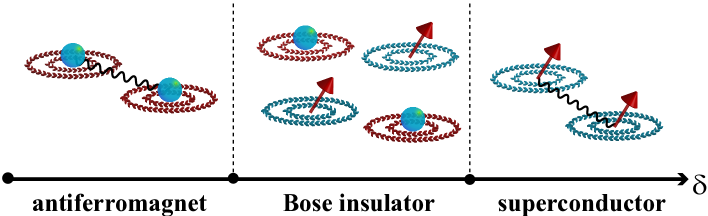
Figure 3: (Color online) Quantum phase diagram of underdoped Mott insulators. The ball (in blue) and the arrow (in red) stand for the holon and spinon, respectively. The vortex, in red (blue), surrounding a holon (spinon) arises from the spinon (holon) condensate. The wavy line stands for the confinement.

V.1 Superconducting phase

We first study the regime far away from zero doping, where the superconducting phase is formed. In this phase, the spinons are confined while holons deconfined. Such peculiar confinement properties of spinons (holons) are intrinsic to the onset of holon superfluids. Upon decreasing the doping, the spinons undergo a deconfinement transition. Correspondingly, the system loses its superconducting long-ranged order.

V.1.1 Logarithmic spinon confinement and holon deconfinement

In this regime, the holon Lagrangian ${\cal L}_{h}$ is minimized upon the formation of superfluid, justifying the superconducting phase (with a density $n_{h}=(2t_{h}-\lambda^{h})/u_{1}$). In the presence of a holon superfluid, a uniform “magnetic field” is formed and minimally couples to the motion of spinons [cf. Eq. (67)]. Consequently, a Landau-type gap is opened in the spinon spectrum and spin excitations are suppressed. For sufficiently large doping, these spin excitations may be ignored and the functional integral over the spin degree of freedom $\Psi$ is frozen at state composing of the so-called resonance valence bond (RVB) pairs. As such, the functional integral over $\Psi$ accounts only for an irrelevant overall factor, and the Wilson loop, $W^{h}[{\cal C}]$ , is simplified to

$$W^{h}[{\cal C}]\propto\sum_{\{\mathscr{N}^{s,h}\}}\int D[A^{s},A^{h}]D[h^{\dagger},h]\exp\left\{-\sum_{x}\left[{\cal L}_{h}+\frac{i}{\pi}\epsilon^{\mu\nu\lambda}\left(A^{s}_{{\mu}}-2\pi\mathscr{N}^{s}_{\mu}\right)d_{\nu}\left(A^{h}_{\lambda}-2\pi\mathscr{N}^{h}_{\lambda}\right)-iA^{h}_{\mu}J_{\cal C}^{\mu}\right]\right\}.$$ (86)

To proceed further, we separate the spatial components of the gauge field, $A^{h}_{\alpha}-2\pi\mathscr{N}^{h}_{\alpha}$, into two parts. The first, denoted as $\bar{A}^{h}_{\alpha}$ , is the background component which satisfies

$$\epsilon^{0\alpha\beta}d_{\alpha}\bar{A}^{h}_{\beta}=\pi n_{h}$$ (87)

and therefore, is imaginary time-dependent. (To be consistent with this condition it is necessary that $\mathscr{N}^{s}_{0}$ must be uniform in the lattice plane.) The second is the fluctuation component. Then, we factorize the holon field as

$$h(x)=|h|e^{-i\theta_{1}(x)}\,,$$ (88)

substitute it into Eq. (86) and make the change of variable: $A_{\alpha}^{s}\rightarrow A_{\alpha}^{s}-d_{\alpha}\theta_{1}$ . Integrating out the matter field $h$ with the help of saddle point approximation and summing up the integer field $\mathscr{N}^{h}_{\mu}$ , we obtain

$$W^{h}[{\cal C}] \propto \sum_{\{\mathscr{N}^{s}\}}\int D[A^{s},A^{h}]\exp\left\{-\sum_{x}\left[\frac{i}{\pi}\epsilon^{\alpha\nu\lambda}\left(A_{\alpha}^{s}-2\pi\mathscr{N}^{s}_{\alpha}\right)d_{\nu}A^{h}_{\lambda}+\frac{i}{\pi}\epsilon^{0\alpha\beta}A^{s}_{0}d_{\alpha}A_{\beta}^{h}\right]\right\}\exp\left\{i\sum_{x}A^{h}_{\mu}J_{\cal C}^{\mu}\right\}$$ (89)

$$\qquad\qquad\qquad\qquad\times\exp\left\{-\frac{1}{2u_{1}}\sum_{x}\left(A_{0}^{s2}+2n_{h}t_{h}u_{1}\,A_{\alpha}^{s2}\right)\right\}\,.$$

Here, the integral variable $A_{\alpha}^{h}$ stands for the fluctuation component of the corresponding gauge field. In deriving this equation we have used the facts that summing up the fluctuating flux gives a vanishing result, and that $\mathscr{N}^{s}_{0}$ is uniform in the lattice plane. Notice that an irrelevant factor $e^{i\sum_{x}\bar{A}_{\alpha}^{h}J_{\cal C}^{\alpha}}$ has been omitted. Importantly, the first term in the first exponent above suggests that in the presence of holon superfluids, $\mathscr{N}_{\alpha}^{s}$ is identical to the integer fields introduced by the Villain’s approximation Villain . Notice that $\theta_{1},\,d_{\mu}\theta_{1}\in[-\pi,+\pi]$ is non-singular, and the singular component of the phase fluctuations is very captured by (the spatial components of) the integer field. Integrating out the $A^{s}$ fields gives

$$W^{h}[{\cal C}]\propto\sum_{\{\mathscr{N}^{s}\}}\int D[A^{h}]\exp\left\{-\sum_{x}\left[\frac{u_{1}}{2\pi^{2}}\left(\epsilon^{0\mu\nu}d_{\mu}A_{\nu}^{h}\right)^{2}+\frac{1}{4\pi^{2}n_{h}t_{h}}\left(\epsilon^{\alpha\mu\nu}d_{\mu}A_{\nu}^{h}\right)^{2}-iA^{h}_{\mu}\left(J_{\cal C}^{\mu}+2\epsilon^{\mu\nu\alpha}d_{\nu}\mathscr{N}^{s}_{\alpha}\right)\right]\right\}\,.$$ (90)

From this we see that the dynamics of the fluctuations of the gauge field $A^{h}$ displays emergent Lorentz symmetry with a “speed of light” $c_{1}=\sqrt{2n_{h}t_{h}u_{1}}$ . By introducing the following rescaling:

$$(d_{0}/c_{1},d_{x},d_{y})\rightarrow d_{\mu},\qquad(A_{0}^{h}/c_{1},A^{h}_{x},A^{h}_{y})\rightarrow A^{h}_{\mu},\qquad(c_{1}J_{\cal C}^{0},J_{\cal C}^{x},J_{\cal C}^{y})\rightarrow J_{\cal C}^{\mu},\qquad c_{1}\mathscr{N}^{s}_{\alpha}\rightarrow\mathscr{N}^{s}_{\alpha},$$ (91)

we rewrite Eq. (90) as

$$W^{h}[{\cal C}] \propto \sum_{\{\mathscr{N}^{s}\}}\int D[A^{h}]\exp\left\{-\sum_{x}\left[\frac{1}{4e_{1}^{2}}\left(F_{\mu\nu}^{h}\right)^{2}-iA^{h}_{\mu}\left(J_{\cal C}^{\mu}+2\epsilon^{\mu\nu\alpha}d_{\nu}\mathscr{N}^{s}_{\alpha}\right)\right]\right\}$$ (92)

$$\rightarrow \sum_{\{\mathscr{N}^{s}\}}\int D[A^{h}]\exp\left\{-\sum_{x}\left[\frac{1}{4e_{1}^{2}}\left(F_{\mu\nu}^{h}\right)^{2}-iA^{h}_{\mu}J_{\cal C}^{\mu}-2iA^{h}_{0}\epsilon^{0\alpha\beta}d_{\alpha}\mathscr{N}^{s}_{\beta}\right]\right\}\,.$$

Here, $F_{\mu\nu}^{h}=d_{\mu}A^{h}_{\nu}-d_{\nu}A^{h}_{\mu}$ is the Maxwell tensor and $e_{1}^{2}=\pi^{2}/u_{1}$ is the squared “bare charge”. In obtaining the second line we have used the fact, $d_{0}\mathscr{N}^{s}_{\alpha}=0$ , at zero temperature.

If no phase vortices are present, i.e., $2\pi\epsilon^{0\alpha\beta}d_{\alpha}\mathscr{N}^{s}_{\beta}=0$ , Eq. (92) is simplified to

$$W^{h}[{\cal C}]\propto\int D[A^{h}]\exp\left\{-\sum_{x}\left[\frac{1}{4e_{1}^{2}}\left(F_{\mu\nu}^{h}\right)^{2}-iA^{h}_{\mu}J_{\cal C}^{\mu}\right]\right\}\,.$$ (93)

As we will show in Appendix B, it can be further reduced to (Here, we restore the original unit.)

$$W^{h}[{\cal C}]\propto e^{-TV^{s}(R)},\qquad V^{s}(R)=\frac{(e_{1}c_{1})^{2}}{2\pi}\ln\frac{R}{R^{*}_{1}}=\pi n_{h}t_{h}\ln\frac{R}{R^{*}_{1}}$$ (94)

for $T\rightarrow\infty$, where $R^{*}_{1}$ is the ultraviolet cutoff. Notice that the coefficient of the potential, i.e., $\pi n_{h}t_{h}$ , does not depend on the strength of the on-site repulsive interaction. Eq. (94) suggests that an external dipole undergoes logarithmic confinement and has important consequences: (i) The presence of a pair of free phase vortices of the holon superfluid, carrying opposite vorticity, is energetically unfavorable which is consistent with the simplification above; (ii) In the presence of spin excitations (right, Fig. 3), this dipole may mimic a pair of spinons with opposite or identical polarizations. In the latter case, a phase vortex with a vorticity of $\pm 2\pi$ may be excited from the background and bound to a spinon of flux $\mp\pi$, reversing the sign of the bare topological charge of the spinon accordingly, i.e., $\mp\pi\rightarrow\pm\pi$ . That is, a pair of spin excitations must be logarithmically confined.

We turn now to calculate $W^{s}[{\cal C}]$ . To this end we may ignore the fluctuation component of the gauge field $A_{\alpha}^{h}$ . Following the same procedures of deriving Eq. (89) from Eq. (86), we find (Here, we do not rescale the gauge field and $d_{\mu}$ .)

$$W^{s}[{\cal C}]\propto\sum_{\{\mathscr{N}^{s}\}}\int D[A^{s},A_{0}^{h}]\exp\left\{-\sum_{x}\left[\frac{1}{2u_{1}}\left(A_{0}^{s2}+n_{h}t_{h}u_{1}A_{\alpha}^{s2}\right)+\frac{i}{\pi}\,\epsilon^{0\alpha\beta}\left(A^{s}_{{\alpha}}-2\pi\mathscr{N}^{s}_{\alpha}\right)d_{\beta}A^{h}_{0}-iA^{s}_{\mu}J_{\cal C}^{\mu}\right]\right\}\,,$$ (95)

where we have used the fact that $\theta_{1}(x)$ is non-singular giving $d_{\alpha}d_{\beta}\theta_{1}=d_{\beta}d_{\alpha}\theta_{1}$ and $\sum_{x}d_{\mu}\theta_{1}J_{\cal C}^{\mu}=0$ . The functional integrals over the temporal and spatial components of $A^{s}$ are factorizable, i.e.,

$$W^{s}[{\cal C}] \propto \int D[A_{0}^{s}]\exp\left\{-\sum_{x}\left(\frac{1}{2u_{1}}A_{0}^{s2}-iA^{s}_{0}J_{\cal C}^{0}\right)\right\}$$ (96)

$$\times\int D[A_{\alpha}^{s},A_{0}^{h}]\sum_{\{\mathscr{N}^{s}\}}\exp\left\{-\sum_{x}\left[\frac{1}{2}n_{h}t_{h}A_{\alpha}^{s2}+\frac{i}{\pi}\epsilon^{\alpha\beta 0}\left(A^{s}_{{\alpha}}-2\pi\mathscr{N}^{s}_{\alpha}\right)A^{h}_{0}-iA^{s}_{\alpha}J_{\cal C}^{\alpha}\right]\right\}$$

$$\equiv \exp\left\{-\left[f_{1}\left(\frac{c_{1}T}{\sqrt{n_{h}t_{h}}}\right)+f_{2}\left(\frac{R}{\sqrt{n_{h}t_{h}}}\right)\right]\right\}\,,$$

with the scaling function $f_{1}$ ($f_{2}$) independent of $R$ ($T$). This is none but a (holon) deconfinement law – insensitive to the details of the scaling functions $f_{1,2}$ – as expected by holon superfluids. Shortly we will see that this Wilson loop is not critical at the spinon deconfinement critical point.

V.1.2 Non-BCS nature of superconductivity

Let us subject the system to a small magnetic field with a total flux $\Phi^{e}$ . Consider an area ${\cal A}$ on the spatial plane that is enclosed by a sufficiently large loop. Since in the ground state, spinons are confined into RVB pairs and do not contribute a net flux, integrating out the $A_{0}^{h}$ field leads to

$$\sum_{x\in{\cal A}}\Psi^{\dagger}\Sigma\Psi\equiv\Phi^{e}\quad{\rm mod}\,2\pi\,.$$ (97)

As we explained above, the left-hand side is quantized with a quanta $\pi$ . This implies in turn that Eq. (97) is none but the quantization condition of the external magnetic flux, i.e., $\Phi^{e}=n(hc/2e),\,n\in\mathbb{Z}$ in the full unit unit . However, this quantization is intrinsic to the topological spin excitations and differs in the nature from its counterpart in BCS superconductivity. In fact, in the absence of the external magnetic field, i.e., $\Phi^{e}=0$ , a single spin carrying a flux of $\pm\pi$ cannot be excited otherwise Eq. (97) is violated. Instead, spins are excited in pairs, constituting a spin-$0$ (or spin-$1$) excitation. However, in the presence of the external magnetic field, i.e., $\Phi^{e}\neq 0$ , a single spin can be excited provided it is nucleated at the magnetic vortex core. Moreover, as a result of the spin rotation symmetry, both polarizations are possible Weng02 .

We then examine the static electric conductivity. As mentioned above, in the absence of the external magnetic field, spinons are excited in pairs. If two spinons have identical polarization, they cannot mobile because they are always bound to a (local) phase vortex of holon superfluids, as shown in Sec. V.1.1. If two spinons have opposite polarization, as shown in Sec. V.1.1, they undergo logarithmic confinement. Therefore, neither of these spinon pairs supports spinon transport, i.e., $\sigma_{s}=0$. On the other hand, since holons undergo Bose condensation, the holon conductivity is infinite, i.e., $\sigma_{h}=\infty$. From the composition rule (85) we then obtain $\sigma_{e}=\infty$. It is important that according to composition rule, the establishment of superconductivity relies crucially on a vanishing spinon conductivity $\sigma_{s}$ which arises from the spinon confinement. In other words, it suggests that the disappearance of superconductivity has to be associated with the spinon deconfinement, where $\sigma_{s}$ no longer vanishes – a fact reflecting the non-BCS nature of superconductivity that we will see in Sec. V.3.

V.2 Antiferromagnetic phase

Now we study the regime adjacent to zero doping, where the antiferromagnetic phase is formed. In this phase, the holons are confined while spinons deconfined. Such peculiar confinement properties of spinons (holons) are intrinsic to the onset of spinon superfluids. Upon increasing the doping, the holons undergo a deconfinement transition. Correspondingly, the system loses its antiferromagnetic long-ranged order. The analysis below is largely parallel to those of Sec. V.1. Therefore, we shall only sketch the main steps.

V.2.1 Logarithmic holon confinement and spinon deconfinement

Consider the case where holons are sufficiently dilute and the holon Lagrangian is thereby ignored. As a result,

$$W^{s}[{\cal C}]\propto\sum_{\{\mathscr{N}^{s,h}\}}\int D[A^{s},A^{h}]D[\Psi^{\dagger},\Psi]\exp\left\{-\sum_{x}\left[{\cal L}_{s}+\frac{i}{\pi}\epsilon^{\mu\nu\lambda}\left(A^{s}_{{\mu}}-2\pi\mathscr{N}^{s}_{\mu}\right)d_{\nu}\left(A^{h}_{\lambda}-2\pi\mathscr{N}^{h}_{\lambda}\right)-iA^{s}_{\mu}J_{\cal C}^{\mu}\right]\right\}\,.$$ (98)

The antiferromagnetism is justified by the existence of homogeneous saddle points, denoted as $\Psi_{0}$ ,i.e.,

$$\frac{\delta S}{\delta\Psi^{\dagger}}\bigg{|}_{\Psi_{0},\,d\Psi_{0}=0}=0\,.$$ (99)

In Appendix C we will show that (i) the saddle point has the structure as $\Psi_{0}=(\sqrt{n_{\uparrow}}e^{i\theta_{\uparrow}},\sqrt{n_{\downarrow}}e^{i\theta_{\downarrow}},\sqrt{n_{\downarrow}}e^{i\theta_{\downarrow}},\sqrt{n_{\uparrow}}e^{i\theta_{\uparrow}})^{T}$ with $n_{\sigma}$ and $\theta_{\sigma}$ homogeneous in spacetime and $n_{\uparrow}+n_{\downarrow}=(2J_{s}-\lambda_{s})/(2u_{2})$ ; and (ii) the total spin polarization vanishes, i.e.,

$$\Psi_{0}^{\dagger}\Sigma\Psi_{0}=0\,,$$ (100)

as a manifestation of antiferromagnetism.

Next we wish to integrate out the spinon field. To this end we factorize the $\Psi$ field as

$$\Psi(x)=\left(\begin{array}[]{c}\sqrt{n_{\uparrow}+\frac{\delta n_{1}(x)+\delta n_{2}(x)}{2}}\,e^{i\theta_{2}(x)/2}\\ \sqrt{n_{\downarrow}+\frac{\delta n_{3}(x)-\delta n_{4}(x)}{2}}\,e^{-i\theta_{2}(x)/2}\\ \sqrt{n_{\downarrow}+\frac{\delta n_{3}(x)+\delta n_{4}(x)}{2}}\,e^{i\theta_{2}(x)/2}\\ \sqrt{n_{\uparrow}+\frac{\delta n_{1}(x)-\delta n_{2}(x)}{2}}\,e^{-i\theta_{2}(x)/2}\\ \end{array}\right)$$ (105)

and insert it into Eq. (98). The phase field $\theta_{2}(x)$ generates the Goldstone mode. Furthermore, because of Eq. (100) the background component of the gauge field $A_{\alpha}^{s}-2\pi\mathscr{N}_{\alpha}^{s}$ vanishes. With the help of the saddle point approximation we obtain from Eq. (98)

$$W^{s}[{\cal C}] \propto \sum_{\{\mathscr{N}^{h}\}}\int D[A^{s},A^{h}]D[\delta n,\theta_{2}]\exp\left\{-\sum_{x}\left[\frac{i}{\pi}\epsilon^{\alpha\nu\lambda}\left(A_{\alpha}^{h}-2\pi\mathscr{N}^{h}_{\alpha}\right)d_{\nu}A^{s}_{\lambda}+\frac{i}{\pi}\epsilon^{0\alpha\beta}A^{h}_{0}d_{\alpha}A_{\beta}^{s}\right]\right\}\exp\left\{i\sum_{x}A^{s}_{\mu}J_{\cal C}^{\mu}\right\}$$ (106)

$$\qquad\qquad\qquad\qquad\times\exp\left\{-\sum_{x}\left[-iA_{0}^{h}(\delta n_{2}+\delta n_{4})+2J_{s}(n_{\uparrow}+n_{\downarrow})(d_{\alpha}\theta_{2}-A_{\alpha}^{h})^{2}\right]\right\}$$

$$\qquad\qquad\qquad\qquad\times\exp\left\{\sum_{x}\left[\frac{J_{s}}{4}\left(\delta n_{1}^{2}+\delta n_{3}^{2}-\delta n_{2}^{2}-\delta n_{4}^{2}\right)-\frac{u_{2}}{2}\left(\delta n_{1}+\delta n_{3}\right)^{2}\right]\right\}\,.$$

Again $\theta_{2}(x)$ is non-singular and instead, the integer field $\mathscr{N}_{\alpha}^{h}$ characterizes the singular part of the phase field namely the phase vortex of the spinon superfluid. Integrating out $\delta n$ and $\theta$ gives

$$W^{s}[{\cal C}]\propto\sum_{\{\mathscr{N}^{h}\}}\int D[A^{h},A^{s}]\exp\left\{-\sum_{x}\left[\frac{J_{s}}{8}\left(A_{0}^{h2}+16(n_{\uparrow}+n_{\downarrow})A_{\alpha}^{h2}\right)+\frac{i}{\pi}\left(A^{h}_{{\mu}}-2\pi\epsilon^{\alpha\nu\lambda}\mathscr{N}^{h}_{\alpha}\right)d_{\nu}A^{s}_{\lambda}-ia^{s}_{\mu}J_{\cal C}^{\mu}\right]\right\}\,.$$ (107)

This result is identical to Eq. (89) upon making the replacement: $u_{1}^{-1}\rightarrow J_{s}/4,2n_{h}t_{h}u_{1}\rightarrow 16(n_{\uparrow}+n_{\downarrow})$ for the parameters and $h\rightarrow s,s\rightarrow h$ for the superscripts. Translating Eq. (94) into the present context, we find

$$W^{s}[{\cal C}]\propto e^{-TV^{h}(R)},\qquad V^{h}(R)=2\pi(n_{\uparrow}+n_{\downarrow})J_{s}\ln\frac{R}{R^{*}_{2}}$$ (108)

for $T\rightarrow\infty$ . Here, $R^{*}_{2}$ is the ultraviolet cutoff. Notice that here the Lorentz symmetry emerges but with a different “speed of light”. The squared “bare charge” is also different from that of the superconducting phase.

Eq. (108) also suggests that an external dipole undergoes logarithmic confinement and has important consequences as follows. (i) The presence of a pair of free phase vortices of the spinon superfluid, carrying opposite vorticity, is energetically unfavorable. (ii) In the presence of holon excitations, a phase vortex with a vorticity of $-2\pi$ may be excited from the background and bound to a holon of flux $+\pi$, reversing the sign of the bare topological charge of the holon accordingly (the so-called “anti-holon”), i.e., $\pi\rightarrow-\pi$. Eq. (108) then implies that such a holon–anti-holon pair is bound together via the logarithmic confinement (left, Fig. 3). In other words, two holons are bound to a phase vortex of the spinon superfluid with a vorticity of $-2\pi$ .

We turn now to calculate $W^{h}[{\cal C}]$. Similar to Eq. (95), we find

$$W^{h}[{\cal C}]\propto\sum_{\{\mathscr{N}^{h}\}}\int D[A^{h},A_{0}^{s}]\exp\left\{-\sum_{x}\left[\frac{J_{s}}{8}\left(A_{0}^{h2}+16(n_{\uparrow}+n_{\downarrow})A_{\alpha}^{h2}\right)+\frac{i}{\pi}\,\epsilon^{0\alpha\beta}\left(A^{h}_{{\alpha}}-2\pi\mathscr{N}^{h}_{\alpha}\right)d_{\beta}A^{s}_{0}-iA^{h}_{\mu}J_{\cal C}^{\mu}\right]\right\}\,,$$ (109)

which gives

$$W^{h}[{\cal C}]\propto\exp\left\{-\left[f_{1}\left(\frac{c_{2}T}{\sqrt{n_{\uparrow}+n_{\downarrow}}}\right)+f_{2}\left(\frac{R}{\sqrt{n_{\uparrow}+n_{\downarrow}}}\right)\right]\right\}\,.$$ (110)

It suggests spinon deconfinement as expected by spinon superfluids, insensitive to the details of the scaling functions $f_{1,2}$ . As we will see below, this Wilson loop in non-critical at the holon deconfinement critical point.

V.2.2 Unconventional antiferromagnetism

Similar to the discussions in Sec. V.1.2, the antiferromagnetism ($\delta\neq 0$) here is unconventional. Let us subject the system to a spin twist generated by an external gauge field $A^{\prime}_{\alpha}$ . Since in the ground state, holons and anti-holons are confined in pairs and do not contribute a net flux, integrating out the $A_{0}^{s}$ field leads to

$$\sum_{x\in{\cal A}}h^{\dagger}h\equiv\sum_{x\in{\cal A}}\epsilon^{0\alpha\beta}d_{\alpha}A^{\prime}_{\beta}\quad{\rm mod}\,2\pi$$ (111)

dual to Eq. (97). Since the left-hand side is quantized (with the same quanta $\pi$), this implies a dual quantization condition: the external flux generating the spin twist may penetrate into the antiferromagnet only if it takes the value of $n\pi,\,n\in\mathbb{Z}$ . This quantization is intrinsic to the topological holon excitations. In fact, in the absence of the external spin twist, a single holon cannot appear in the excitation spectrum otherwise Eq. (111) is violated. Instead, the holon and the anti-holon are excited in pairs, constituting a charge-$2$ bosonic excitation. However, in the presence of the spin twist, a single (anti-)holon can be excited provided it is nucleated at the center of the spin twist.

For the static electric transport, we note that in the absence of external spin twist, the holon and the anti-holon are excited in pairs. According to Sec. V.2.1, such pair is bound to a phase vortex of spinon superfluids. Since the latter is localized in space, (As such, the spontaneous translational symmetry breaking appears.) $\sigma_{h}=0$ . From the composition rule (85) we then find that the antiferromagnetic phase is insulating, i.e., $\sigma_{e}=0$ . It is important that such a property of electric transport is intrinsic to the holon confinement and, therefore, persists to some finite doping – the holon deconfinement critical point. This is in sharp contrast to previous theories Lee06 where the superconducting phase was found to be pushed all the way down to zero doping. Finally, it should be noted that without the integer field $\mathscr{N}^{h}_{\alpha}$ describing the spinon phase vortex, such an antiferromagnetic insulating phase cannot be established.

V.3 Bose insulating phase

The qualitatively different behaviors of $W^{h}[{\cal C}]$ described by Eqs. (94) and (110) suggest a critical doping $\delta_{2}$ , at which $W^{h}[{\cal C}]$ – as a function of $\delta$ – is non-analytic. This is the spinon deconfinement quantum critical point. Likewise, the expressions of Eqs. (96) and (108) for $W^{s}[{\cal C}]$ suggest another critical doping $\delta_{1}$, at which $W^{s}[{\cal C}]$ is non-analytic. This is the holon deconfinement quantum critical point. The mechanisms underlying these two quantum critical points – the disappearance of the superconducting or the antiferromagnetic long-ranged order, are independent. Thus, $\delta_{1}\neq\delta_{2}$ generally. Since the confinement of holons (spinons) is a consequence of spinon (holon) condensation, the case of $\delta_{1}>\delta_{2}$ is ruled out. That is, spinons and holons cannot be confined simultaneously. Instead, we have $\delta_{1}<\delta_{2}$ generally. As such, there is an intermediate phase separating the antiferromagnetic and the superconducting phases.

Indeed, this is a novel phase where both matter fields undergo condensation characterized by the field $\Psi_{0}$ ($h_{0}$). It should be contrasted to the antiferromagnetic (superconducting) phase where only the spinon (holon) field $\Psi$ ($h$) is condensed. The fields $\Psi_{0}\,,\,h_{0}$ are determined by the following self-consistent equations:

$$\frac{\delta S}{\delta h^{\dagger}}\bigg{|}_{h_{0},\,d_{0}h_{0}=0}=0\,,\quad\frac{\delta S}{\delta\Psi^{\dagger}}\bigg{|}_{\Psi_{0},\,d_{0}\Psi_{0}=0}=0\,,$$ (112)

$$\epsilon^{0\alpha\beta}d_{\alpha}\left(A_{\beta}^{s}-2\pi\mathscr{N}^{s}_{\beta}\right)=\pi\Psi^{\dagger}_{0}\Sigma\Psi_{0}\,,$$ (113)

$$\epsilon^{0\alpha\beta}d_{\alpha}\left(A_{\beta}^{h}-2\pi\mathscr{N}^{h}_{\beta}\right)=\pi h^{\dagger}_{0}h_{0}\,.$$ (114)

In general, the field $\Psi_{0}$ ($h_{0}$) has an amplitude inhomogeneous in space. In the Wilson loops (69) the functional integral over $A_{\alpha}^{s}\,,\,\mathscr{N}^{s}_{\alpha}$ ($A_{\alpha}^{h}\,,\,\mathscr{N}^{h}_{\alpha}$) is dominated by the small fluctuations (denoted by $a_{\alpha}^{s,h}$) near the background configurations satisfying Eqs. (113) and (114). Taking Eqs. (112)-(114) into account, we rewrite Eq. (69) as (To make the formula compact we denote $A_{0}^{s,h}$ as $a_{0}^{s,h}$ .)

$$W^{s,h}[{\cal C}] \propto \int D[a^{s},a^{h}]D[h^{\dagger},h,\Psi^{\dagger},\Psi]\exp\left\{-\sum_{x}\left[{\cal L}_{h}|_{a_{0}^{s}=0}-ia_{0}^{s}(h^{\dagger}h-h_{0}^{\dagger}h_{0})\right]\right\}$$ (115)

$$\times\exp\left\{-\sum_{x}\left[{\cal L}_{s}|_{a_{0}^{h}=0}-ia_{0}^{h}(\Psi^{\dagger}\Sigma\Psi-\Psi_{0}^{\dagger}\Sigma\Psi_{0})\right]\right\}\exp\left\{-\sum_{x}\left[\frac{i}{\pi}\epsilon^{\mu\nu\lambda}a_{\mu}^{s}d_{\nu}a_{\lambda}^{h}-ia^{s,h}_{\mu}J_{\cal C}^{\mu}\right]\right\}\,.$$

The first (second) exponent involves merely $a^{s}$ ($a^{h}$). It is important that integrating out the holon (spinon) field leads to an effective action of $a^{s}$ ($a^{h}$) which is massive. (This can be readily seen by observing that a spacetime-independent $a^{s}$ ($a^{h}$) cannot be absorbed into the functional integral over $h$ ($\Psi$) and as such, the effective action of a homogeneous $a^{s}$ ($a^{h}$) must not vanish.) Therefore, the residual mutual statistical interaction between gauge field fluctuations, of order ${\cal O}(d_{\mu})$ , is negligible, and Eq. (115) is simplified to

$$W^{s,h}[{\cal C}] \propto \int D[a^{s},a^{h}]D[h^{\dagger},h,\Psi^{\dagger},\Psi]\exp\left\{-\sum_{x}\left[{\cal L}_{h}|_{a_{0}^{s}=0}-ia_{0}^{s}(h^{\dagger}h-h_{0}^{\dagger}h_{0})\right]\right\}$$ (116)

$$\times\exp\left\{-\sum_{x}\left[{\cal L}_{s}|_{a_{0}^{h}=0}-ia_{0}^{h}(\Psi^{\dagger}\Sigma\Psi-\Psi_{0}^{\dagger}\Sigma\Psi_{0})\right]\right\}\exp\left[i\sum_{x}a^{s,h}_{\mu}J_{\cal C}^{\mu}\right]\,.$$

Integrating out the matter fields then gives

$$W^{s,h}[{\cal C}]\propto\int D[a^{s},a^{h}]\exp\bigg{\{}-\sum_{x}\bigg{[}\frac{1}{2u_{1}}\left(a_{0}^{s2}+(c_{1}a_{\alpha}^{s})^{2}\right)+\frac{J_{s}}{8}\left(a_{0}^{h2}+(c_{2}a_{\alpha}^{h})^{2}\right)-ia^{s,h}_{\mu}J_{\cal C}^{\mu}\bigg{]}\bigg{\}}\,.$$ (117)

From this equation we see that the functional integrals over the temporal and spatial components of $a^{s}$ ($a^{h}$) can be factorized. As a result, we obtain

$$W^{s}[{\cal C}] \propto \exp\left\{-\left[\tilde{f}_{1}\left(\frac{c_{1}T}{\sqrt{n_{h}t_{h}}}\right)+\tilde{f}_{2}\left(\frac{R}{\sqrt{n_{h}t_{h}}}\right)\right]\right\}\,,$$

$$W^{h}[{\cal C}] \propto \exp\left\{-\left[\tilde{f}_{1}\left(\frac{c_{2}T}{\sqrt{n_{\uparrow}+n_{\downarrow}}}\right)+\tilde{f}_{2}\left(\frac{R}{\sqrt{n_{\uparrow}+n_{\downarrow}}}\right)\right]\right\}\,,$$ (118)

where the new scaling functions $\tilde{f}_{1,2}$ are independent of $R$ ($T$). Insensitive to the details of these scaling functions, the Wilson loops (118) indicate that an external pair composed of holon and anti-holon or spinons with opposite polarizations undergoes deconfinement (middle, Fig. 3). Comparing these two expressions with Eqs. (96) and (110), we find that $W^{s}[{\cal C}]$ ($W^{h}[{\cal C}]$) is indeed non-critical at the spinon (holon) deconfinement critical point.

The spinon and the holon deconfinement have far reaching consequences. First, both the long-ranged antiferromagnetic and superconducting order no longer exist in this phase. Second, recent studies by one of us Weng11 have shown that due to the spinon and the holon condensation, the phase of the electron operator is disordered, indicating the existence of a disordered gapless fermionic mode. As a result, this phase is compressible. (The present Bose insulator may be considered as a new example of the zero-temperature compressible quantum matters proposed recently Sachdev11 .) In other words, the holon (charge) density may be continuously tuned from $\delta_{1}$ to $\delta_{2}$ . Finally, alluding to $\sigma_{s,h}=\infty$ arising from spinon (holon) condensation, we find that this phase is also insulating, $\sigma_{e}=0$ , from the composition rule (85).

VI Conclusions

The $t$-$J$ model (on a bipartite lattice) displays a non-perturbative sign structure, the so-called phase string effect. With this effect being taken into full account an electron is necessarily fractionalized into two bosonic constituents, the holon (the charge degree of freedom) and the spinon (the spin degree of freedom). Each constituent is a topological object and carries a $\pi$ flux. The latter mediates a compact $U(1)$ gauge field, $A^{s}_{\mu}$ ($A^{h}_{\mu}$), minimally couples to the motion of holons (spinons)–the so-called mutual statistical interaction. In this work, the exact phase string effect is refined in terms of the lattice field theory. Based on this field theory, a pair of unconventional order parameters namely the Wilson loops $W^{s,h}[{\cal C}]$ is introduced. These two unconventional order parameters describe the holon (spinon) confinement-deconfinement property and suffice to characterize the phase diagram of the $t$-$J$ model in the underdoped regime. We further establish a general composition rule for the electric transport, which expresses the electric conductivity in terms of the spinon and the holon conductivities.

The lattice field theory and the general composition rule are applied to study the quantum phase diagram. In the antiferromagnetic regime, where the doping is sufficiently small, spinons undergo deconfinement while holons are confined, leading to an (electrically) insulating phase with long range antiferromagnetic order. Whereas for sufficiently large doping, holons undergo deconfinement while spinons are confined, leading to a superconducting phase. (Further analysis of such a superconducting phase unveils that this is a $d$-wave superconductor and possesses fermionic Bogoliubov qusiparticles Weng11 .) We find that $W^{s}[{\cal C}]$ ($W^{h}[{\cal C}]$) displays non-analyticity at some doping $\delta_{1}$ ($\delta_{2}$ with $\delta_{1}<\delta_{2}$), where the system undergoes a holon (spinon) deconfinement quantum phase transition. Most strikingly, we find that between the antiferromagnetic and the superconducting phase, there is a novel phase, the Bose insulating phase. In this phase, despite of spinon and holon condensation, no long range orders occur and the system is also electrically insulating. These results inform profoundly non-Landau-Ginzburg-Wilson nature of quantum phase transitions in the $t$-$J$ model. We remark that different from the earlier field theoretic formulation KQW05 , the present lattice field theory is compact, and the compactness of the emergent $U(1)$ gauge fields is essential to the formation of the antiferromagnetic and the Bose insulating phase. Finally, we should emphasize that the present theory is not limited to the quantum case. Applications to the finite temperature case are of fundamental importance and of great interests, which we leave for future studies.

Note added. After this paper was submitted, we became aware of the works by Tesanovic and co-workers Tesanovic08 . These authors also found that the duality between the superconducting and the antiferromagnetic phase dooms to lead to an intermediate insulating phase. Although this scenario is similar to the quantum phase diagram presented here, the intermediate phase reported in these papers has very different nature.

Appendix A Alternative derivation of mutual Chern-Simons term

In Sec. III.1, in deriving the mutual Chern-Simons term the gauge fields $A^{s}_{\alpha}$ ($A^{h}_{\alpha}$) are essentially considered as “external” parameters as the holon (spinon) motion concerned [cf. Eqs. (20) and (21)]. These external parameters are then subject to the self-consistent constraints (25). In this Appendix, we follow Ref. KQW05, to give an alternative derivation of the mutual Chern-Simons term.

The starting point is the observation that $A^{s,h}_{\alpha}$ constitute the canonically conjugated pair. Indeed, with the help of the constraint $\mathscr{F}_{A^{h}}=0$ [cf. Eq. (25)], the holon current conservation law may be rewritten as

$$d_{0}\left(\frac{1}{\pi}\,\epsilon^{0\alpha\beta}\,d_{\alpha}A^{h}_{\beta}\right)+\sum_{\alpha}\,d_{\alpha}\left(-\frac{\delta{\cal H}}{\delta A^{s}_{\alpha}}\right)=0\,.$$ (119)

Exchanging the order of the derivatives of the first term, we obtain

$$\frac{1}{\pi}\left(d_{x}d_{0}\,A^{h}_{y}-d_{y}d_{0}\,A^{h}_{x}\right)+d_{x}\left(-\frac{\delta{\cal H}}{\delta A^{s}_{x}}\right)+d_{y}\left(-\frac{\delta{\cal H}}{\delta A^{s}_{y}}\right)=0\,,$$ (120)

which gives

$$\frac{1}{\pi}\,d_{0}\,A^{h}_{y}=\frac{\delta{\cal H}}{\delta A^{s}_{x}}\,,\qquad\frac{1}{\pi}\,d_{0}\,A^{h}_{x}=-\frac{\delta{\cal H}}{\delta A^{s}_{y}}\,.$$ (121)

From the spinon current conservation law we may obtain two similar equations. Together with Eq. (121) they justify the canonically conjugated relation:

$$\Pi^{h}_{x}=-\frac{1}{\pi}\,A^{s}_{y}\,,\qquad\Pi^{h}_{y}=\frac{1}{\pi}\,A^{s}_{x}\,.$$ (122)

Passing to the path integral representation, instead of Eq. (28), we obtain Eq. (45) directly.

Appendix B Derivation of logarithmic confinement

In this Appendix we prove Eq. (94). Throughout this Appendix we set $c_{1}=1$ , and without the loss of generality, we have set the four corners of the timelike rectangle to be $(0,0,0),(R,0,0),(R,0,T),(0,0,T)$. Notice that Eq. (93) is gauge invariant and to further proceed we must fix the gauge. Under the Feynmann gauge Peskin , it becomes

$$W^{h}[{\cal C}]\propto\int D[A^{h}]\exp\left\{-\sum_{x}\left[\frac{1}{2e_{1}^{2}}\left(d_{\mu}A_{\nu}^{h}\right)^{2}-ia^{h}_{\mu}J_{\cal C}^{\mu}\right]\right\}\,.$$ (123)

Since we are interested physics at large scales, we pass to the continuum limit, obtaining the gauge field propagator read

$$D_{\mu\nu}({\bf x}-{\bf x}^{\prime},\tau-\tau^{\prime})=\int\frac{d\omega d^{2}k}{(2\pi)^{3}}e^{i{\bf k}\cdot({\bf x}-{\bf x}^{\prime})-i\omega(\tau-\tau^{\prime})}\frac{e_{1}^{2}\delta_{\mu\nu}}{\omega^{2}+|{\bf k}|^{2}}=\frac{1}{4\pi}\frac{e_{1}^{2}\delta_{\mu\nu}}{\sqrt{|{\bf x}-{\bf x}^{\prime}|^{2}+|\tau-\tau^{\prime}|^{2}}}.$$ (124)

Then, because of $T\gg R$ diagrams with a propagator line starting from the rectangular sides in the spatial direction are penalized by (some power of) a small factor $R/T\ll 1$ and thereby are negligible. As a result, to the leading order expansion in $e_{1}^{2}$ Eq. (123) is dominated by the two diagrams shown in Fig. 4. By ignoring the irrelevant overall numerical factor, which is the same for both diagrams, they give

$${\rm diagram\,(a)} = -2\times\frac{1}{2}\int D[A^{h}]\int_{0}^{T}d\tau d\tau^{\prime}A^{h}_{0}(0,0,\tau)A^{h}_{0}(0,0,\tau^{\prime})\exp\left[-\frac{1}{2e_{1}^{2}}\sum_{x}\left(d_{\mu}A_{\nu}^{h}\right)^{2}\right]$$ (125)

$$= -\int_{0}^{T}d\tau d\tau^{\prime}D_{00}(0,0,\tau-\tau^{\prime})=-\frac{e_{1}^{2}}{4\pi}\int_{0}^{T}d\tau d\tau^{\prime}\frac{1}{|\tau-\tau^{\prime}|}$$

$$= -\frac{Te_{1}^{2}}{2\pi}\int_{0}^{1}dx\ln\frac{xT}{\tau^{*}},$$

with $\tau^{*}$ an ultraviolet cutoff in the imaginary time direction, and

$${\rm diagram\,(b)} = 2\times\frac{1}{2}\int D[A^{h}]\int_{0}^{T}d\tau d\tau^{\prime}A^{h}_{0}(0,0,\tau)A^{h}_{0}(R,0,\tau^{\prime})\exp\left[-\frac{1}{2e_{1}^{2}}\sum_{x}\left(d_{\mu}A_{\nu}^{h}\right)^{2}\right]$$ (126)

$$= \int_{0}^{T}d\tau d\tau^{\prime}D_{00}(R,0,\tau-\tau^{\prime})=\frac{e_{1}^{2}}{4\pi}\int_{0}^{T}d\tau d\tau^{\prime}\frac{1}{\sqrt{R^{2}+|\tau-\tau^{\prime}|^{2}}}$$

$$= \frac{e_{1}^{2}}{4\pi}\int_{0}^{T}d\tau\ln\frac{T-\tau+\sqrt{(T-\tau)^{2}+R^{2}}}{-\tau+\sqrt{\tau^{2}+R^{2}}}=\frac{Te_{1}^{2}}{4\pi}\int_{0}^{1}dx\ln\frac{x+\sqrt{x^{2}+(R/T)^{2}}}{-x+\sqrt{x^{2}+(R/T)^{2}}}$$

$$\stackrel{{\scriptstyle T\rightarrow\infty}}{{\simeq}} \frac{Te_{1}^{2}}{2\pi}\int_{0}^{1}dx\ln\frac{2Tx}{R},$$

respectively. Notice that in the first line of Eqs. (125) and (126), the factor $2$ is the combinatorial factor. Adding these two terms together, we find

$${\rm diagram\,(a)}+{\rm diagram\,(b)}\stackrel{{\scriptstyle T\rightarrow\infty}}{{\simeq}}-\frac{Te_{1}^{2}}{2\pi}\ln\frac{R}{2\tau^{*}}\equiv-\frac{Te_{1}^{2}}{2\pi}\ln\frac{R}{R^{*}_{1}},$$ (127)

which is Eq. (94), with $R^{*}_{1}=2\tau^{*}$ an ultraviolet cutoff in the spatial direction. Notice that these two diagrams suffer logarithmical divergences in $T$ , which, however, cancel each other exactly upon adding them together.

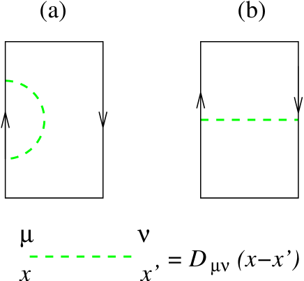
Figure 4: Diagrams contributing to the Wilson loop for $T\rightarrow\infty$.

Appendix C Spinon superfluids

From Eqs. (67) and (99) we obtain

$${\cal M}|_{d_{0}=A^{h}=0}\Psi_{0}+u_{2}(\Psi_{0}^{\dagger}\Psi_{0})\Psi_{0}=0\,.$$ (128)

If we re-arrange the components of the vector as follows: $\Psi_{0}\equiv(\Psi_{01},\,\Psi_{02},\,\Psi_{03},\,\Psi_{04})^{T}\rightarrow(\Psi_{01},\,\Psi_{04},\,\Psi_{02},\,\Psi_{03})^{T}$ , and further introduce two two-component vectors, $z_{\sigma},\,\sigma=\uparrow,\,\downarrow$ , defined in the sector introduced by the sublattice structure, then $\Psi_{0}=(z_{\uparrow}^{T},\,z_{\downarrow}^{T})^{T}$ . (This two-component structure is defined in the spin sector.) Consequently, we may rewrite Eq. (128) as

$$\left(\begin{array}[]{cc}\lambda^{s}&-2J_{s}\\ -2J_{s}&\lambda^{s}\\ \end{array}\right)z_{\uparrow}+u_{2}(z_{\uparrow}^{\dagger}z_{\uparrow}+z_{\downarrow}^{\dagger}z_{\downarrow})z_{\uparrow}=0\,,$$ (131)

$$\left(\begin{array}[]{cc}\lambda^{s}&-2J_{s}\\ -2J_{s}&\lambda^{s}\\ \end{array}\right)z_{\downarrow}+u_{2}(z_{\uparrow}^{\dagger}z_{\uparrow}+z_{\downarrow}^{\dagger}z_{\downarrow})z_{\downarrow}=0\,.$$ (134)

Solving these two equations we obtain

$$z_{\sigma}=\sqrt{n_{\sigma}}e^{i\theta_{\sigma}}\left(\begin{array}[]{c}1\\ 1\\ \end{array}\right)\,,\qquad n_{\uparrow}+n_{\downarrow}=(2J_{s}-\lambda_{s})/(2u_{2})\,,$$ (137)

where $n_{\sigma}$ and $\theta_{\sigma}$ are homogeneous in spacetime. This saddle point solution gives $z_{\sigma}^{\dagger}\Sigma_{3}z_{\sigma}=0$ with $\Sigma_{3}={\rm diag}(1,-1)$ defined on the sector introduced by the sublattice structure. As a result, we find that the total spin polarization vanishes namely Eq. (100).

References

- (1) T. Senthil, A. Vishwanath, L. Balents, S. Sachdev, and M. P. A. Fisher, Science 303, 1490 (2004).
- (2) T. Senthil, L. Balents, S. Sachdev, A. Vishwanath, and M. P. A. Fisher, Phys. Rev. B 70, 144407 (2004).
- (3) L. Balents, L. Bartosch, A. Burkov, S. Sachdev, and K. Sengupta, Phys. Rev. B 71, 144508 (2005).
- (4) R. K. Kaul, A. Kolezhuk, M. Levin, S. Sachdev, and T. Senthil, Phys. Rev. B 75, 235112 (2007).
- (5) P. W. Anderson, Science 235, 1196 (1987); S. A. Kivelson, D. S. Rokhsar, and J. P. Sethna, Phys. Rev. B 35, 8865 (1987); Z. Zou and P. W. Anderson, Phys. Rev. B 37, 627 (1988).
- (6) P. A. Lee, N. Nagaosa, and X. G. Wen, Rev. Mod. Phys. 78, 17 (2006).
- (7) T. Senthil and M. P. A. Fisher, Phys. Rev. B 62, 7850 (2000).
- (8) S. Sachdev, Rev. Mod. Phys. 75, 913 (2003).
- (9) N. P. Ong, Y. Wang, S. Ono, Y. Ando, and S. Uchida, Annalen der Physik 13, 9 (2004); Y. Wang, S. Ono, Y. Onose, G. Gu, Y. Ando, Y. Tokura, S. Uchida, and N. P. Ong, Science 299, 86 (2003).
- (10) See: for example, T. Hanaguri, C. Lupien, Y. Kohsaka, D.-H. Lee, M. Azuma, M. Takano, H. Takagi, and J. C. Davis, Nature 430, 1001 (2004).
- (11) J. Zaanen and B. J. Overbosch, Phil. Trans. R. Soc. A 369, 1599 (2011).
- (12) Z. Y. Weng, D. N. Sheng, Y. C. Chen, and C. S. Ting, Phys. Rev. B 55, 3894 (1997); K. Wu, Z. Y. Weng, and J. Zaanen, Phys. Rev. B 77, 155102 (2008).
- (13) P. Ye, C. S. Tian, X. L. Qi, and Z. Y. Weng, Phys. Rev. Lett. 106, 147002 (2011).
- (14) See: Z. Y. Weng, Intl. J. Mod. Phys. B 21, 773 (2007) for a review.
- (15) W. Marshall, Proc. R. Soc. London A 232, 48 (1955).
- (16) The spacetime lattice constant, the Planck’s constant, the speed of light in vacuum, and the electron charge are set to unity.
- (17) C. Xu and S. Sachdev, Phys. Rev. B 79, 064405 (2009).
- (18) V. M. Galitskii, G. Gafel, M. P. A. Fisher, and T. Senthil, Phys. Rev. Lett. 95, 077002 (2005).
- (19) M. C. Diamantini, P. Sodano, and C. A. Trugenberger, J. Phys. A: Math. Gen. 39, L253 (2006).
- (20) S. P. Kou, X. L. Qi, and Z. Y. Weng, Phys. Rev. B 71, 235102 (2005).
- (21) J. Villain, J. Physics (Paris) 36, 581 (1975).
- (22) A. Altland and B. Simons, Condensed matter field theory (Cambridge, UK, 2006).
- (23) See: e.g., P. Giovannangeli and C. P. Korthals Altes, Nucl. Phys. B 608, 203 (2001).
- (24) V. N. Muthukumar and Z. Y. Weng, Phys. Rev. B 65, 174511 (2002).
- (25) M. E. Peskin and D. V. Schroeder, An introduction to quantum field theory (Perseus, Cambridge, 1995).
- (26) Z. Y. Weng, arXiv:1105.3027 (2011).
- (27) L. Huijse and S. Sachdev, arXiv:1104.5022 (2011).
- (28) Z. Tesanovic, Nature Physics 4, 408 (2008); A. Melikyan and Z. Tesanovic, Phys. Rev. B 71, 214511 (2005).