Seebeck effect in dilute two-dimensional electron systems: temperature dependencies of diffusion and phonon-drag thermoelectric powers

Abstract

Considering screeening of electron scattering interactions in terms of the finite-temperature STLS theory and solving the linearized Boltzmann equation (with no appeal to a relaxation time approximation), we present a theoretical analysis of the low-temperature Seebeck effect in two-dimensional semiconductors with dilute electron densities. We find that the temperature ($T$) dependencies of the diffusion and phonon-drag thermoelectric powers ($S_{d}$ and $S_{g}$) can no longer be described by the conventional simple power-laws. As temperature increases, $|S_{d}|/T$ decreases when $T\gtrsim 0.1\varepsilon_{F}$ ($\varepsilon_{F}$ is the Fermi energy), while $|S_{g}|$ first increases and then falls, resulting a peak located at a temperature between Bloch-Grüneisen temperature and $\varepsilon_{F}$.

I Introduction

Heat generation with increasing density of integrated electronic devices is one of the serious restrictions blocking the further development of conventional electronics. To overcome this obstacle, there have been proposals to use heat to storage and transport information. Such an intriguing concept provides hope of discovering new physics and new green technology, stimulating a great deal of theoretical and experimental investigation. Recently, two new subfields associated with heat electronics have emerged, namely ”Phononics”Wang and Li (2008a) and ”Spin Caloritronics”.Bauer et al. (2010) Phononics is devoted to the use of heat current to perform computational operations and many heat devices, such as heat diodes,Segal (2008a); *Hu2006; *Li2005; *Segal2005; *Li2004; *Terraneo2002 heat transistorsLo et al. (2008); *Segal2008; *Li2006, thermal memoryWang and Li (2008b) etc., have been proposed and/or constructed. Spin Caloritronics concerns on the motion of magnetization or of electron spin induced by heat or a temperature gradient.Bauer et al. (2010) In this field, many phenomena, such as a spin Seebeck effect,Uchida et al. (2008); *Uchida2010; *Jaworski2010 thermodynamic control of magnetization in ferromagneto-nonmagnetic structures, [Forareview; seeforexample; ]Johnson2010 etc. have been reported.

To use heat in electronics, the conventional method is usually based on thermoelectric effects, which convert a temperature gradient to electric voltage. Among them, the Seebeck effect (SE), initially discovered in metals by T. Seebeck in the 1820s,Seebeck (1823, 1825) is widely used for thermoelectric generation and for temperature sensing. The first observations of SE in bulk semiconductors, such as GermaniumFrederikse (1953); Geballe and Hull (1954) and Silicon,Geballe and Hull (1955) were reported in the 1950’s. With the recent development of technology in the fabrication of semiconductor microstructures, investigations of thermoelectric effects in two-dimensional electron gases (2DEG) have been carried out both experimentallyObloh et al. (1984); Nicholas et al. (1984); Fletcher et al. (1985); Davidson et al. (1986); Fletcher et al. (1986); Obloh et al. (1986); Ruf et al. (1988); Fletcher et al. (1988); Ying et al. (1994); Fletcher et al. (1994); Bayot et al. (1995); Tieke et al. (1996); Fletcher et al. (1997); Miele et al. (1998); Fletcher et al. (1998); Fletcher (2002); Maximov et al. (2004); Zhang et al. (2004); Rafael et al. (2004); Chickering et al. (2009, 2010) and theoretically.Girvin and Jonson (1982); Zawadzki and Lassnig (1984); Nicholas (1985); Cantrell and Butcher (1987a, b); Kubakaddi et al. (1987); Kundu et al. (1987); Lyo (1988); Basak and Kar (1989); Kubakaddi et al. (1989); Okuyama and Tokuda (1990); Karavolas et al. (1990); Karavolas and Butcher (1991); X. L. Lei (1994); Zianni et al. (1994); Khveshchenko (1996); Wu et al. (1996); Cooper et al. (1997); Khveshchenko and Reizer (1997); Tsaousidou et al. (1999); Karavolas and Triberis (2001); Kundu and Datta (2001); Tsaousidou et al. (2001); Sankeshwar et al. (2005); Sergeev et al. (2005)

It is well known that, in thermoelectric power (TEP), which is the main characteristic quantity of SE, there are two components; namely, diffusion thermopower, $S_{d}$, and phonon-drag thermopower, $S_{g}$. At relatively low temperature, the diffusion process in the Seebeck effect has been expected to be dominant since the electron-phonon scattering is relatively weak.Nicholas et al. (1984); Obloh et al. (1984); Fletcher et al. (1985); Davidson et al. (1986); Obloh et al. (1986) However, a careful analysis of experimental data indicates that phonon-drag in 2DEGs also plays an important role even at temperature $T<10$ K.Ruf et al. (1988); Fletcher et al. (1988, 1986); Wu et al. (1996); Okuyama and Tokuda (1990); Kubakaddi et al. (1989); Lyo (1988); Kundu et al. (1987); Kubakaddi et al. (1987); Cantrell and Butcher (1987b, a); Nicholas (1985) Furthermore, there have also been studies of a sign change of diffusion TEP in a Si-MOSFET,Karavolas et al. (1990); Karavolas and Butcher (1991) and of the effects of weak localization on TEP, Miele et al. (1998); Fletcher (2002); Rafael et al. (2004) as well as the TEP of composite-fermions,Chickering et al. (2010); Karavolas and Triberis (2001); Tsaousidou et al. (1999); Khveshchenko and Reizer (1997); Tieke et al. (1996); Bayot et al. (1995); Khveshchenko (1996); Ying et al. (1994) and oscillation of TEP in low magnetic field,Fletcher et al. (1998); Zhang et al. (2004); Maximov et al. (2004) etc.

To understand the microscopic mechanisms in SE, it is necessary to separate $S_{d}$ and $S_{g}$ from the total TEP that is measured. One way to do this is to analyze the temperature dependencies of $S_{d}$ and $S_{g}$. In the absence of phonon-phonon scattering in the phonon relaxation process, low-temperature $S_{g}$ vs $T$ behavior has been taken to be of the form: $S_{g}\propto\Lambda T^{n}$ with $\Lambda$ as the phonon mean free path and $n=3$ or $n=4$ for dirty or clean samples respectively.Khveshchenko and Reizer (1997); Fletcher (2002) The diffusion TEP has often been assumed to vary linearly with temperature.Fletcher et al. (1997) However, Sankeshwar, et al. showed that the inelastic feature of electron-phonon scattering may result in a nonlinear temperature dependence of $S_{d}$ in relatively clean 2D samples in the Bloch-Grüneisen (BG) regime, i.e. $T<T_{\rm BG}$ [the BG temperature $T_{\rm BG}\equiv 2k_{F}u_{s\lambda}$ with $u_{s\lambda}$ as the phonon velocity in branch $\lambda$ is about 5 K for a 2DEG with typical density $n_{s}\sim 10^{11}$ cm^-2].Sankeshwar et al. (2005) A few experiments were devoted to the direct measurement of diffusion TEP.Fletcher et al. (1994); Ying et al. (1994); Chickering et al. (2009) Ying, et al. observed pure diffusion TEP only in the case $T\leq 0.2$ K.Ying et al. (1994) Recently, using hot electron thermocouple structures, the diffusion TEP has been directly detected by Chickering, et al. when $T<2$ K.Chickering et al. (2009)

It should be noted that the simple power-laws of $S_{d}$ and $S_{g}$ vs $T$, obtained previously, were derived on the basis of a relaxation time approximation (RTA), which is valid when $T,T_{\rm BG}\ll\varepsilon_{F}$. Recently, motivated by the observation of a so-called metal-insulator transition in resistivity vs temperature, clean undoped heterojunctions with electron density $n_{s}$ as low as $n_{s}\leq 10^{10}$ cm^-2 have been studied extensively.Zhou et al. (2010); Lilly et al. (2003); [Forareview; seeforexample; ]Spivak2010 In these systems, $T$ and $T_{\rm BG}$ are comparable with the Fermi energy even at low temperature and therefore deviations of $S_{d}$ and $S_{g}$ vs $T$ from the conventional results are expected to be observed.

In this paper, within the framework of Boltzmann equation, we present a theoretical investigation on thermoelectric effects in 2D electron GaAs/AlGaAs systems with carrier densities $n_{s}=0.23\sim 1.06\times 10^{10}$ ${\rm cm}^{-2}$. To account for the screening of scattering interactions in a 2DEG with such low $n_{s}$, the finite-temperature Singwi-Tosi-Land-Sjolander (STLS) theory, a scheme beyond random phase approximation (RPA), is employed.Singwi et al. (1968); Schweng and B hm (1994) Furthermore, to carefully treat inelastic electron-phonon scattering, the Boltzmann equation is solved with no appeal to a relaxation time approximation, using an energy expansion method. Das Sarma and Hwang have already presented a qualitative explanation of experimental observations of resistivity in a 2DEG with such dilute $n_{s}$ by means of a Boltzmann equation combined with RPA-screened electron-impurity scattering.Das Sarma and Hwang (2004, 2003, 1999) In the present paper, performing numerical calculations with STLS screening appropriate to low carrier density, we find that the temperature dependencies of $S_{d}$ and $S_{g}$ in dilute 2D systems are significantly different from those in the high-electron-density limit. When temperature increases, $|S_{d}|/T$ no longer remains unchanged: it decreases for $T\gtrsim 0.1\varepsilon_{F}$. In our calculation of phonon-drag TEP vs temperature, a peak appears: $|S_{g}|$ first increases and then falls as temperature increases.

The paper is organized as follows. In Sec. II, an energy expansion method for solving the Boltzmann equation beyond the RTA is presented along with the self-consistent finite-temperature STLS theory. Numerical investigation of the temperature dependencies of diffusion and phonon-drag TEPs for various dilute electron densities are exhibited in Sec. III. Our results and conclusions are summarized in Sec. IV. In the Appendix, we also provide analytical results for $S_{d}$ and $S_{g}$ vs $T$ in the high-electron-density limit, obtained by the energy expansion method.

II Theoretical Considerations

II.1 Electron and phonon Boltzmann equations

When a two-dimensional electron with momentum ${\bm{p}}\equiv(p\cos\varphi_{\bm{p}},p\sin\varphi_{\bm{p}})$ and energy $\varepsilon_{\bm{p}}=\frac{p^{2}}{2m^{*}}$ ($m^{*}$ is the effective electron mass) is subjected to a weak electric field $\bm{E}$ and a thermal gradient $\bm{\nabla}T$, its kinetic motion can be described in terms of a nonequilibrium distribution function, $f_{\bm{p}}$, which is determined by a linearized Boltzmann equation of form

$$\left(e{\bm{E}}\cdot{\bm{v}}_{\bm{p}}+\frac{\varepsilon_{\bm{p}}-\mu}{T}{\bm{\nabla}}T\cdot{\bm{v}}_{\bm{p}}\right)\frac{\partial f_{0}(\varepsilon_{\bm{p}})}{\partial\varepsilon_{\bm{p}}}=I_{\rm scatt}.$$ (1)

Here, $\mu$ is the chemical potential, $T$ is the lattice temperature, $f_{0}(\varepsilon_{\bm{p}})=\{\exp[(\varepsilon_{\bm{p}}-\mu)/T]+1\}^{-1}$ is the equilibrium electron distribution function and ${\bm{v}}_{\bm{p}}\equiv{\bm{\nabla}}_{\bm{p}}\varepsilon_{\bm{p}}={\bm{p}}/m^{*}$ is the electron velocity. In Eq. (1), $I_{\rm scatt}$ is the scattering term due to electron-impurity and electron-phonon interactions and it can be written as $I_{\rm scatt}=I_{\rm imp}+I_{\rm ph}$. $I_{\rm imp}$ represents the contribution to $I_{\rm scatt}$ from electron-impurity scattering:

$$I_{\rm imp}=-2\pi\sum_{\bm{q}}|\widetilde{U}_{\bm{q}}|^{2}\delta(\varepsilon_{\bm{p}}-\varepsilon_{{\bm{p}}-{\bm{q}}})\left(f_{\bm{p}}-f_{{\bm{p}}-{\bm{q}}}\right),$$ (2)

while $I_{\rm ph}$ is associated with the electron-phonon interaction:

$$I_{\rm ph} = -{2\pi}\sum_{{\bm{Q}},\lambda,\pm}|\widetilde{M}_{{\bm{Q}}\lambda}|^{2}\delta(\varepsilon_{{\bm{p}}\pm{\bm{q}}}-\varepsilon_{{\bm{p}}}\mp\Omega_{{\bm{Q}}\lambda})$$ (3)

$$\times\left[N_{{\bm{Q}}\lambda}^{\pm}f_{\bm{p}}(1-f_{\bm{p}\pm\bm{q}})-N_{{\bm{Q}}\lambda}^{\mp}f_{\bm{p}\pm\bm{q}}(1-f_{\bm{p}})\right].$$

In Eqs. (2) and (3), $\widetilde{U}_{\bm{q}}$ is the electron-impurity scattering potential, $\widetilde{M}_{{\bm{Q}}\lambda}$ is the matrix element for interaction between the 2D electrons and 3D phonons, and $N^{\pm}_{{\bm{Q}}\lambda}\equiv N_{{\bm{Q}}\lambda}+\frac{1}{2}\mp\frac{1}{2}$. $\Omega_{{\bm{Q}}\lambda}$ and $N_{{\bm{Q}}\lambda}$, respectively, are the energy and number of nonequilibrium phonons with three-dimensional momentum ${\bm{Q}}\equiv({\bm{q}},q_{z})=(q_{x},q_{y},q_{z})$ in branch $\lambda$.

Since the temperature gradient may drive the phonons out of equilibrium, $N_{{\bm{Q}}\lambda}$ in Eq. (3) differs from the number of equilibrium phonons, $n_{{\bm{Q}}\lambda}\equiv\left[\exp(\Omega_{{\bm{Q}}\lambda}/T)-1\right]^{-1}$, and it is determined by the Boltzmann equation for phonons:

$$\frac{dN_{{\bm{Q}}\lambda}}{dt}=\left(\frac{\partial N_{{\bm{Q}}\lambda}}{\partial t}\right)_{\rm d}+\left(\frac{\partial N_{{\bm{Q}}\lambda}}{\partial t}\right)_{\rm ep}+\left(\frac{\partial N_{{\bm{Q}}\lambda}}{\partial t}\right)_{\rm bp}.$$ (4)

Here, $\left(\frac{\partial N_{{\bm{Q}}\lambda}}{\partial t}\right)_{\rm d}$ is the drift term, taking the form

$$\left(\frac{\partial N_{{\bm{Q}}\lambda}}{\partial t}\right)_{\rm d}=-{\bm{u}}_{\bm{Q}\lambda}\cdot{\bm{\nabla}}N_{{\bm{Q}}\lambda},$$ (5)

with ${\bm{u}}_{\bm{Q}\lambda}$ as the phonon velocity. Note that, in the present paper, the magnitudes of ${\bm{u}}_{\bm{Q}\lambda}$ are assumed to be independent of $\bm{Q}$ and they are denoted by $u_{s\lambda}$ (longitudinal and transverse acoustic phonons are denoted by $u_{sl}$ and $u_{st}$, respectively). $\left(\frac{\partial N_{{\bm{Q}}\lambda}}{\partial t}\right)_{\rm bp}$ is the relaxation term due to the boundary and phonon-phonon scatterings, written as

$$\left(\frac{\partial N_{{\bm{Q}}\lambda}}{\partial t}\right)_{\rm bp}=-\left(\frac{1}{\tau_{\rm bs}}+\frac{1}{\tau_{\rm pp}}\right)\left(N_{{\bm{Q}}\lambda}-n_{{\bm{Q}}\lambda}\right),$$ (6)

with $\tau_{\rm bs}$ as the relaxation time due to boundary scattering, $1/\tau_{\rm bs}=u_{\bm{Q}\lambda}/\Lambda$,Okuyama and Tokuda (1990) and $\tau_{\rm pp}$ as the relaxation time due to phonon-phonon scattering, $1/\tau_{\rm pp}=A_{\lambda}T^{3}\Omega_{\bm{Q}\lambda}^{2}$.Herring (1954); Callaway (1991) $\left(\frac{\partial N_{{\bm{Q}}\lambda}}{\partial t}\right)_{\rm ep}$ is the phonon scattering rate due to the electron-phonon interaction, as given by

$$\left(\frac{\partial N_{{\bm{Q}}\lambda}}{\partial t}\right)_{\rm ep} = -\frac{2\pi}{L}g_{s}|\widetilde{M}_{{\bm{Q}}\lambda}|^{2}\sum_{{\bm{p}},\pm}\left\{\pm\delta(\varepsilon_{\bm{p}}-\varepsilon_{{\bm{p}}\pm{\bm{q}}}\pm\Omega_{{\bm{Q}}\lambda})\right.$$ (7)

$$\times\left.N^{\pm}_{{\bm{Q}}\lambda}f_{\bm{p}}(1-f_{{\bm{p}}\pm{\bm{q}}})\right\},$$

with $g_{s}$ as the spin degeneracy and $L$ as the sample size along the direction perpendicular to the 2D sheet. In the case of a weak temperature gradient, Eq. (5) can be solved analytically and the steady-state number of nonequilibrium phonons can be written as

$$N_{{\bm{Q}}\lambda}=n_{{\bm{Q}}\lambda}-\tau_{{\rm p}\lambda}{\bm{u}}_{\bm{Q}\lambda}\cdot{\bm{\nabla}}T\frac{\partial n_{{\bm{Q}}\lambda}}{\partial T}.$$ (8)

Here, $1/\tau_{{\rm p}\lambda}\equiv 1/\tau_{{\rm bs}}+1/\tau_{{\rm pp}}+1/\tau_{\rm ep}$ and $\tau_{\rm ep}$ is the phonon relaxation time due to electron-phonon scattering, taking the form

$$\frac{1}{\tau_{\rm ep}}=\frac{2\pi g_{s}}{L}\sum_{\bm{p}}|\widetilde{M}_{{\bm{Q}}\lambda}|^{2}\delta(\varepsilon_{{\bm{p}}-{\bm{q}}}-\varepsilon_{\bm{p}}+\Omega_{{\bm{Q}}\lambda})[f_{0}(\varepsilon_{{\bm{p}}-{\bm{q}}})-f_{0}(\varepsilon_{\bm{p}})].$$ (9)

II.2 Energy-expansion method to solve electron Boltzmann equation

To solve the electron Boltzmann equation, Eq. (1), we assume that the nonequilibrium distribution function $f_{\bm{p}}$ takes the form

$$f_{\bm{p}}=f_{0}(\varepsilon_{\bm{p}})+g_{\bm{p}}\left[-\frac{\partial f_{0}(\varepsilon_{\bm{p}})}{\partial\varepsilon_{\bm{p}}}\right],$$ (10)

with $g_{\bm{p}}$ as an unknown function. In previous studies, when electron-optical-phonon scattering can be ignored at low temperature, $g_{\bm{p}}$ is usually obtained using the relaxation time approximation (RTA). Obviously, RTA is valid only in the high-electron-density limit. In the present paper, in order to study diffusion and phonon-drag TEPs for relatively low electron density, we follow the idea proposed by Allen for an investigation of transport in metals,Allen (1978) which assumes that $g_{\bm{p}}$ can be expanded in terms of basis functions $\chi_{Jn}({\bm{p}})$:

$$g_{\bm{p}}=\sum_{J,n}C_{Jn}\chi_{Jn}({\bm{p}}),$$ (11)

with $C_{Jn}$ as the coefficients of expansion. In a 2D system with a parabolic dispersion relation, the functions $\chi_{Jn}({\bm{p}})$ can be written as

$$\chi_{Jn}(\bm{p})=4\pi F_{J}({\bm{p}})\frac{\eta_{n}(\varepsilon_{\bm{p}})}{p}.$$ (12)

Here, $F_{J}(\bm{p})$ are the basis functions for the expansion of $g_{\bm{p}}$ with respect to the angle of the momentum vector $\bm{p}$, and they can be chosen as sine or cosine functions of multiples of the angle $\varphi_{\bm{p}}$. $\eta_{n}(\varepsilon)$ are $n$-$th$ order polynomials in electron energy $\varepsilon$ and they are orthogonal with respect to the weight function $-\partial f_{0}(\varepsilon)/\partial\varepsilon$:

$$\int_{0}^{\infty}\left(-\frac{\partial f_{0}(\varepsilon)}{\partial\varepsilon}\right)\eta_{n}(\varepsilon)\eta_{m}(\varepsilon)d\varepsilon=\delta_{nm}.$$ (13)

It is noted that to study the transport in metals, the lower limit of energy integration in Eq. (13) can be assumed to be $-\infty$, since the Fermi energy in metals usually is much larger than the bottom of electron energy band.Allen (1978) However, in three- or two-dimensional semiconductors, the finite bottom of the energy band or subband may affect transport properties, especially at relatively high temperature (or for relatively low electron density). Hence, in Eq. (13), the lower limit of integration is maintained equal to zero. Further, in our study, we assume that $\eta_{n}(\varepsilon)$ take the form

$$\eta_{n}(\varepsilon)=\sum_{m=0}^{n}\alpha_{nm}\varepsilon^{m},$$ (14)

which also differs from that proposed by Allen.Allen (1978) In Eq. (14), the parameters $\alpha_{nm}$ are determined from the orthonormality conditions of $\eta_{n}(\varepsilon)$. In general, they are independent of $\varepsilon$ but may depend on the lattice temperature, as well as on the Fermi energy $\mu$. Note that for $n=0$, $\eta_{0}(\varepsilon)$ is an energy-independent constant: $\eta_{0}(\varepsilon)=\eta_{0}$.

Furthermore, without loss of generality, we assume that the electric field and temperature gradient are applied along the $x$ axis. Thus, in 2D semiconductors with parabolic dispersion, only one term with basis function $F_{J=X}({\bm{p}})=\cos\varphi_{\bm{p}}$ need be considered in the expansion of $g_{\bm{p}}$ with respect to $\varphi_{\bm{p}}$. Multiplying both sides of Eq. (1) by $\chi_{n}({\bm{p}})$ [$\chi_{n}({\bm{p}})\equiv\chi_{n,J=X}({\bm{p}})=4\pi\cos\varphi_{\bm{p}}\eta_{n}(\varepsilon_{\bm{p}})/p$] and performing the summation over ${\bm{p}}$, the linearized Boltzmann equation for electrons can be rewritten as

$$-\frac{eE}{\eta_{0}}\delta_{n0}-\frac{\nabla_{x}T}{T}\sum_{m=0}^{n}\alpha_{nm}\gamma_{m}+\frac{\nabla_{x}T}{T}D_{n}=\sum_{n^{\prime}=0}^{\infty}Q_{nn^{\prime}}C_{n^{\prime}}$$ (15)

with $\gamma_{m}=\int_{0}^{\infty}d\varepsilon(\varepsilon-\mu)\varepsilon^{m}\frac{\partial f_{0}(\varepsilon_{\bm{p}})}{\partial\varepsilon_{\bm{p}}}$. In this equation, the third term on left-hand side is the source of the phonon-drag effect: it describes the interaction between equilibrium electrons and nonequilibrium phonons. In it, $D_{n}$ take the form

$$D_{n} = 2\pi\sum_{{\bm{Q}},{\bm{p}},\lambda,\pm}(\mp 1)|\widetilde{M}_{{\bm{Q}}\lambda}|^{2}\chi_{n}(\varepsilon_{\bm{p}})\delta(\varepsilon_{{\bm{p}}-{\bm{q}}}-\varepsilon_{{\bm{p}}}\mp\Omega_{{\bm{Q}}\lambda})\tau_{{\rm p}\lambda}$$ (16)

$$\times u^{x}_{\bm{Q}\lambda}\frac{\Omega_{\bm{Q}\lambda}}{T}n_{{\bm{Q}}\lambda}(1+n_{{\bm{Q}}\lambda})\left[f_{0}(\varepsilon_{\bm{p}})-f_{0}(\varepsilon_{{\bm{p}}-{\bm{q}}})\right],$$

with $u^{x}_{\bm{Q}\lambda}$ as the $x$ component of ${\bm{u}}_{\bm{Q}\lambda}$. Note that Eq. (16) is derived from Eq. (3) by substituting into it the explicit form of the number of nonequilibrium phonons, i.e. Eq. (8). On right-hand side (r.h.s.) of Eq. (15), $Q_{nn^{\prime}}$ are associated with the scattering term $I_{\rm sc}$ and they can be written as $Q_{nn^{\prime}}=Q_{nn^{\prime}}^{\rm imp}+Q_{nn^{\prime}}^{\rm ph}$ with $Q_{nn^{\prime}}^{\rm imp}$ and $Q_{nn^{\prime}}^{\rm ph}$, respectively, taking the forms ($\varphi_{\hat{\bm{p}\bm{q}}}$ is the angle between $\bm{p}$ and $\bm{q}$)

$$Q_{nn^{\prime}}^{\rm imp} = 16\pi^{3}\sum_{\bm{p},\bm{q}}|\widetilde{U}_{\bm{q}}|^{2}\left[-\frac{\partial f_{0}(\varepsilon_{\bm{p}})}{\partial\varepsilon_{\bm{p}}}\right]\frac{q}{p^{3}}\eta_{n}(\varepsilon_{\bm{p}})\eta_{n^{\prime}}(\varepsilon_{\bm{p}})$$ (17)

$$\times\delta(\varepsilon_{\bm{p}}-\varepsilon_{{\bm{p}}-{\bm{q}}})\cos\varphi_{\hat{\bm{p}\bm{q}}}$$

and

$$Q_{nn^{\prime}}^{\rm ph} = \frac{8\pi^{3}}{m^{*}T}\sum_{\bm{p},\bm{Q},\lambda,\pm}|\tilde{M}_{\bm{Q},\lambda}|^{2}\delta(\varepsilon_{\bm{p}-\bm{q}}-\varepsilon_{\bm{p}}\mp\Omega_{\bm{Q},\lambda})n_{\bm{Q}\lambda}^{\pm}$$ (18)

$$\times f_{0}(\varepsilon_{\bm{p}})[1-f_{0}(\varepsilon_{\bm{p}-\bm{q}})]\frac{1}{\sqrt{\varepsilon_{\bm{p}}}}\eta_{n}(\varepsilon_{\bm{p}})$$

$$\times\left[\frac{\eta_{n^{\prime}}(\varepsilon_{\bm{p}})}{\sqrt{\varepsilon_{\bm{p}}}}-\frac{\eta_{n^{\prime}}(\varepsilon_{\bm{p}-\bm{q}})}{\varepsilon_{\bm{p}-\bm{q}}\sqrt{2m^{*}}}(p-q\cos\varphi_{\hat{\bm{p}\bm{q}}})\right].$$

Thus, the original linearized Boltzmann equation is reduced to Eq. (15), a system of linear equations for $C_{n}$. After $C_{n}$ are determined, the macroscopic charge current can be evaluated through

$${J}_{x}=-g_{s}e\sum_{\bm{p}}\left[-\frac{\partial f_{0}(\varepsilon_{\bm{p}})}{\partial\varepsilon_{\bm{p}}}\right]g_{\bm{p}}{v}_{\bm{p}x}=-g_{s}eC_{0}/\eta_{0}^{2}.$$ (19)

Since there are three driving terms in Eq. (15), its solution, $C_{0}$, can be written as $C_{0}=C_{0}^{(\rm c)}+C_{0}^{(\rm d)}+C_{0}^{(\rm g)}$ with $C_{0}^{(\rm c)}$, $C_{0}^{(\rm d)}$, and $C_{0}^{(\rm g)}$ determined from Eq. (15) in the presence of only the first, the second, or the third driving term, respectively. Obviously, $C_{0}^{(\rm c)}$ is proportional to $E$ and it determines the conductivity as $\sigma=-g_{s}eC_{0}^{(\rm c)}/(\eta_{0}^{2}E)$. $C_{0}^{(\rm d)}$ and $C_{0}^{(\rm g)}$ are proportional to $\nabla_{x}T$ and they are associated with the diffusion and phonon-drag TEPs, respectively: $S_{d}=-g_{s}eC_{0}^{(\rm d)}/(\eta_{0}^{2}\nabla_{x}T\sigma)$ and $S_{g}=-g_{s}eC_{0}^{(\rm g)}/(\eta_{0}^{2}\nabla_{x}T\sigma)$.

We note that such an energy expansion method presented here can also reproduce the previous RTA results in high-electron-density limit. We present a detailed calculation of the high-$n_{s}$ TEP as a function of $T$ in the Appendix, considering screened electron-impurity scattering as well as screened piezoelectric interaction and unscreeened deformation interaction between electron-acoustic phonons. There, the well-known Mott relation is obtained for $S_{d}$, and the lowest-order correction to the Mott formula at low temperature may come not only from electron-impurity scattering but also from the interaction between electrons and acoustic phonons when $T$ lies within the equipartition (EP) regime, $T_{\rm BG}\ll T\ll\varepsilon_{F}$. We also obtain the well-known $T^{4}$ law for $S_{g}$ vs temperature for $T$ within the BG regime. Besides, in the presence of only boundary scattering in the phonon relaxation process, $S_{g}$ is found to be independent of temperature when $T_{\rm BG}\ll T\ll\varepsilon_{F}$.

II.3 Finite-temperature STLS theory

To analyze resistivity as a function of $T$ in dilute 2D systems, it is necessary to clarify the role of screening in electron-impurity and electron-acoustic-phonon scatterings. Using RPA-screened electron-impurity scattering, Das Sarma and Hwang have qualitatively explained the experimental observations in a dilute 2DEG.Das Sarma and Hwang (2004, 2003, 1999) However, in the GaAs systems that we study, the dimensionless Wigner-Seitz density (or interaction) parameter $r_{s}=1/(a_{B}\sqrt{\pi n_{s}})$ [$a_{B}=4\pi\varepsilon_{0}\kappa/(m^{*}e^{2})$ is the effective semiconductor Bohr radius and $\kappa$ is the background dielectric constant] can reach the value $\sim 11.6$ for 2D GaAs with $n_{s}=0.23\times 10^{-10}$ cm^-2. Hence, the local-field correction to RPA is quite important and we therefore use the finite-temperature self-consistent STLS theory here.

Within the framework of the Boltzmann equation approach with interaction screening included, the scattering potential is usually divided by the dielectric function $\varepsilon(q,\omega)$, which takes the form

$$\varepsilon(q,\omega)=1-V_{q}H(q)[1-G(q)]\chi_{0}(q,\omega).$$

Here, $\chi_{0}(q,\omega)$ is the density-density correlation function of the free 2D system, $H(q)$ is the form factor of the electron-electron interaction in the 2D system, and $V_{q}=e^{2}/(2\kappa\varepsilon_{0}q)$ is the 2D Coulomb potential. $G(q)$ is the static local-field factor whose value depends on the approximation that used. In RPA, $G(q)$ is zero, while $G(q)=q/\left(2\sqrt{q^{2}+k_{F}^{2}}\right)$ in Hubbard’s approximation.Jonson (1976) In STLS theory which we use here, the local field factor is determined by the structure factor $S(q)$ through

$$G(q) = -\frac{1}{n_{s}}\sum_{\bm{k}}\frac{{\bm{k}}\cdot{\bm{q}}}{kq}\frac{H(k)}{H(q)}\left[S(|{\bm{k}}-{\bm{q}}|)-1\right].$$ (20)

On the other hand, $S(q)$ is also related to $G(q)$ via

$$S(q)=-\frac{T}{n_{s}}\sum_{n=-\infty}^{\infty}\chi(q,2i\pi nT),$$ (21)

with $\chi(q,i\omega)\equiv\chi_{0}(q,i\omega)/\varepsilon(q,i\omega)$ as the response function. Thus, Eqs. (20) and (21) form a closed system of equations, to be solved self-consistently by iteration.

III Results and Discussion

We carry out numerical calculations to investigate the thermoelectric effect of a dilute 2D electron gas in a GaAs/AlGaAs heterojunction at temperature $T<5$ K. The electron Boltzmann equation is solved by means of the energy expansion method and the screening of scattering is evaluated self-consistently within the framework of the finite-temperature STLS theory. In these calculations, the screened electron-impurity scatterings due to both remote and background impurities are considered. The corresponding scattering potential takes the formLei et al. (1985)

$$|\widetilde{U}_{\bm{q}}|^{2}=|U_{\bm{q}}|^{2}/|\varepsilon(q,0)|^{2}$$ (22)

with $|U_{\bm{q}}|^{2}={V_{q}^{2}}\left[N_{\rm r}{\rm e}^{-2qs}I(q)^{2}+{N_{\rm b}}J(q)/q\right]$, $I(q)$ and $J(q)$ are the form factors, $N_{\rm b}$ is the density of background impurities, and $N_{\rm r}$ represents the density of remote impurities located at distance $s$ from the heterojunction interface on the AlGaAs side.

In regard to the electron-phonon interaction, only acoustic phonons contribute to scattering at low temperature. The corresponding potential can be written as

$$|\widetilde{M}_{\bm{Q}\lambda}|^{2}=|M_{\bm{Q}\lambda}|^{2}|I(iq_{z})|^{2}$$ (23)

with $|M_{\bm{Q}\lambda}|^{2}$ as the matrix element of the electron-phonon interaction in three-dimensional plane-wave representation. In present paper, we consider both the deformation and piezoelectric interactions between electrons and acoustic phonons. It is well known that only the longitudinal acoustic phonon (LA) mode gives rise to deformation scattering with matrix element

$$|M_{{\bm{Q}},{\rm LA}}|_{\rm def}^{2}=\frac{{\Xi}^{2}Q}{2du_{sl}}.$$ (24)

Here, $d$ is the mass density of crystal and $\Xi$ is the shift of the band edge per unit dilation. Both the longitudinal and transverse (TA) acoustic phonons contribute to the piezoelectric interaction. The corresponding scattering matrix elements take the formsLei et al. (1985)

$$|M_{{\bm{Q}},{\rm LA}}|_{\rm piez}^{2}=\frac{32\pi^{2}e^{2}e_{14}^{2}}{\kappa^{2}du_{sl}|\varepsilon(q,\Omega_{\bm{Q},{\rm LA}})|^{2}}\frac{9q_{x}^{2}q_{y}^{2}q_{z}^{2}}{Q^{7}},$$

and

$$|M_{{\bm{Q}},{\rm TA}}|_{\rm piez}^{2} = \frac{32\pi^{2}e^{2}e_{14}^{2}}{\kappa^{2}du_{st}Q^{5}|\varepsilon(q,\Omega_{\bm{Q},{\rm TA}})|^{2}}$$ (25)

$$\times\left(q_{x}^{2}q_{y}^{2}+q_{x}^{2}q_{z}^{2}+q_{y}^{2}q_{z}^{2}-\frac{9q_{x}^{2}q_{y}^{2}q_{z}^{2}}{Q^{2}}\right),$$

with $e_{14}$ as the piezoelectric constant.

In Eqs. (24) and (25), the unscreened form of the electron-acoustic-phonon scattering through deformation potential is used, while the piezoelectric interaction is assumed to be dynamically screened. Such a treatment is based on the fact that these two interactions have completely different origins. It is well known that piezoelectric electron-phonon scattering comes from the Coulomb interaction of electrons in an electric field induced by thermal vibration of atoms, and hence it is effectively screened by electron-electron interactions. However, the deformation scattering mainly results from the overlap of electron wave functions between different atoms in distorted lattices.Bardeen and Shockley (1950) Thus, the deformation interaction between electrons and phonons does not directly relate to the Coulomb interaction, and therefore it is inappropriate to use the screened form for the deformation potential. We note that, employing the unscreened form for the deformation potential with the appropriate parameter $\Xi$, good agreement between theory and experiments has been reached in a previous study on phonon-drag thermoelectric effect.Okuyama and Tokuda (1990)

In our numerical calculations, the parameters are chosen as follows: $\kappa=12.9$, $d=5.31$ g/cm³, $u_{sl}=5.29\times 10^{3}$ m/s, $u_{st}=2.48\times 10^{3}$ m/s, $\Xi=8.5$ eV, $m^{*}=0.067m_{0}$ ($m_{0}$ is free electron mass), $e_{14}=1.41\times 10^{9}$ V/m. Since we are interested in the temperature and electron-density dependencies of the diffusion and phonon-drag TEPs at low temperature ($T\leq 5$ K), the relaxation of phonons due to phonon-phonon scattering can be ignored and only the temperature-independent boundary scattering need be considered. Furthermore, the phonon mean free path is assumed to be $\Lambda=2.42$ mm.Tsaousidou et al. (1999) The truncation of summation in the expansion of $g_{n}$ is estimated by the convergence of the numerical scheme. We find that, for $n_{s}\geq 0.2\times 10^{10}$ cm^-2 and $T\leq 5$ K, $n_{\rm max}=4$ is sufficient to reach the required numerical accuracy.

The low-temperature transport properties depend sensitively on the impurity densities. In the present paper, to obtain results in qualitative agreement with the experimental resistivity data of Ref. Lilly et al., 2003, the density of charges in the depletion layer is chosen to be $N_{\rm dep}=7\times 10^{9}$ cm^-2 and the background impurity density is assumed to be constant: $N_{\rm b}=1\times 10^{18}$ m^-3. The remote impurity density, $N_{\rm r}$, is determined from the mobility at $T=30$ mK by assuming $s=210$ nm. In Fig. 1, we plot the dependencies of resistivity $\rho=1/\sigma$ on temperature for various electron densities. An evident “metal-insulator” transition can be observed: when $T$ increases $\rho$ increases for dense $n_{s}$, while it decreases for dilute $n_{s}$. Such behavior of $\rho$ vs $T$ almost agrees quantitatively with experimental data in the case $1\,{\rm K}\leq T\leq 5\,{\rm K}$ for all $n_{s}$ which were studied (see Fig. 2 in Ref. Lilly et al., 2003). However, in Fig. 1, we do not see the small peaks for intermediate $n_{s}$, which have been observed experimentally.Lilly et al. (2003) This is associated with the fact that the observed small peaks in $\rho$ vs $T$ are the result of weak (or strong) localization, which is ignored in our study.

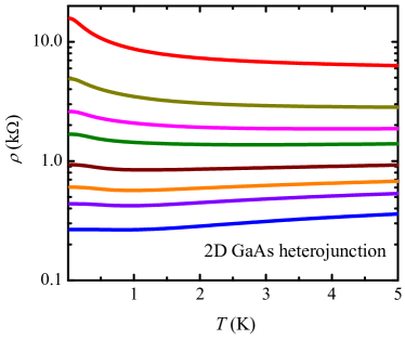
Figure 1: (Color online) Temperature dependencies of resistivity for various densities of electrons (from the top): $n_{s}=0.23$, $0.29$, $0.36$, $0.42$, $0.55$, $0.68$, $0.80$, and $1.06\times 10^{10}$ cm^-2. The remote impurity sheet is assumed to be located at $210$ nm from the interface on AlGaAs side. The density of charges in the depletion layer is assumed to be $N_{\rm dep}=7\times 10^{9}$ cm^-2 and a constant density of background impurities is used: $N_{\rm b}=1\times 10^{18}$ m^-3.

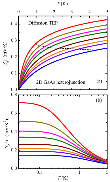
Figure 2: (Color online) Temperature dependencies of (a) $|S_{d}|$ and (b) $|S_{d}|/T$ for various densities of electrons (from the top): $n_{s}=0.23$, $0.29$, $0.36$, $0.42$, $0.55$, $0.68$, $0.80$, and $1.06\times 10^{10}$ cm^-2. The dashed line in Fig. 2(a) indicates the Fermi energy $\varepsilon_{F}$ (in Kelvin).

In Fig. 2, we plot the temperature dependencies of $|S_{d}|$ and $|S_{d}|/T$ in a 2D GaAs heterojunction for various electron densities in the range $0.23\leq n_{s}\leq 1.06\times 10^{10}$ cm^-2. From Fig. 2(a), we see that, with an increase of temperature, $|S_{d}|$ increases. However, this increase is no longer linear. To clearly show the nonlinear dependencies of $S_{d}$ on $T$, the temperature dependencies of $|S_{d}|/T$ for $T\leq 5$ K are plotted in Fig. 2(b). We see that when temperature increases, $|S_{d}|/T$ remains constant only for $T\lesssim 0.1\varepsilon_{F}$. Beyond this regime, $|S_{d}|/T$ decreases with an increase of temperature. Such nonlinear dependence of $S_{d}$ on temperature mainly stems from broadening of the electron distribution function at relatively high temperature.

It should be noted that electron-phonon scattering also may affect $|S_{d}|$ at relatively high temperature. To show this, in Fig. 3, $S_{d}$ vs $T$ is plotted both in the absence and in the presence of electron-phonon interactions. It is clear that the contribution from electron-phonon scattering to $S_{d}$ is important for relatively high $n_{s}$. This is associated with the fact that for dilute $n_{s}$, electron-impurity scattering is so strong that the electron-phonon interaction is relatively unimportant within the temperature regime studied. From Fig. 3, we also see that the magnitude of $S_{d}$ in the presence of electron-phonon interaction is always less than that in the absence of electron-phonon scattering, reflecting the fact that contribution to $|S_{d}|$ from electron-phonon scattering is negative.

Figure 3: (Color online) Effect of electron-phonon scattering on diffusion TEP for $n_{s}=0.23$, $0.42$, and $1.06\times 10^{10}$ cm^-2. The solid and dotted lines indicate $|S_{d}|$ in the presence and in the absence of electron-phonon scattering, respectively.

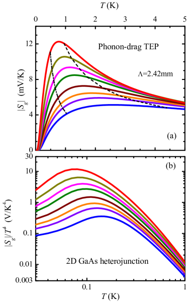
Figure 4: (Color online) Temperature dependencies of (a) $|S_{g}|$ and (b) $|S_{g}|/T^{4}$ for various densities of electrons (from the top): $n_{s}=0.23$, $0.29$, $0.36$, $0.42$, $0.55$, $0.68$, $0.80$, and $1.06\times 10^{10}$ cm^-2. The dotted and dashed lines in Fig. 4(a) indicate $T_{\rm BG}$ and $\varepsilon_{F}$ (in Kelvin), respectively.

In Fig. 4, we plot the temperature dependencies of phonon-drag thermoelectric power for various electron densities. We see that $S_{g}$ vs $T$ for dilute $n_{s}$ is significantly different from that in 2D systems having a dense electron density. It is clear that for relatively high $n_{s}$ (for example in the case $n_{s}=1.06\times 10^{10}$ cm^-2), $|S_{g}|$ increases as $T$ increases and then it saturates at a relatively high temperature. This can be explained qualitatively by means of the asymptotic behavior of $S_{g}$ in high-$n_{s}$ limit, presented in the Appendix: when $T\ll\varepsilon_{F}$, $S_{g}$ first increases with an increase of temperature as $\sim T^{4}$ and it becomes independent of temperature at high temperature. From Fig. 4, we also see that for relatively low $n_{s}$, a peak appears in $|S_{g}|$ vs $T$. The position of peak depends on electron density: the peak moves towards the low temperature side with a decrease of electron density, but it lies always between $T_{\rm BG}$ and $\varepsilon_{F}$.

It should be noted that the appearance of a peak in $S_{g}$ vs $T$ can be understood as the result of competition between (i) broadening of the Fermi distribution function and (ii) decrease of the rate of nonequilibrium phonon production, induced by an increase of temperature. As $T$ increases, the Fermi distribution broadens and dragging electrons out of equilibrium by nonequilibrium phonons is facilitated. As a result, the phonon-drag TEP $|S_{g}|$ increases with increasing $T$. However, as $T$ further increases, the rate of nonequilibrium phonon production induced by a temperature gradient decreases, leading to a decrease of $S_{g}$ with the further increase of $T$. Competition of these two factors results in the nonmonotonic dependence of $S_{g}$ on $T$.

From analysis presented above, it is clear that to observe the nonmonotonic dependence of $|S_{g}|$ on $T$ in the presence of only boundary scattering in the phonon relaxation process, two conditions are required. One condition is that the Fermi energy should be much smaller than the critical temperature at which phonon-phonon scattering is important in phonon-relaxation. In 2D GaAs systems, such a critical temperature is about $10$ K,Wu et al. (1996) leading to an estimate of electron density in a 2D GaAs system for observation of the peak in $S_{g}$ vs $T$ as $n_{s}\lesssim 2.5\times 10^{10}$ cm^-2. The second condition for observation of the peak in $S_{g}$ vs $T$ is that $T_{\rm BG}$ should be comparable with $\varepsilon_{F}$. Otherwise, the peak disappears: as temperature increases, $S_{g}$ monotonically increases and reaches saturation at a relatively high temperature when $T_{\rm BG}\ll\varepsilon_{F}$.

Note that in typical thermoelectric experiments, the measurable quantity is the total thermoelectric power, causing difficulty to separate the diffusion and phonon-drag contributions. In the dilute 2D systems studied here, the phonon-drag TEP is dominant over almost the whole temperature regime $T<5$ K. For example, for $n_{s}=1.06\times 10^{10}$ cm^-2, $|S_{g}|$ exceeds $|S_{d}|$ when $T\gtrsim 0.1$ K. Hence, in the temperature dependence of the total TEP $S=S_{d}+S_{g}$, which is plotted in Fig. 5, the features are almost the same as those in $S_{g}$ vs $T$. Therefore, to observe the nonlinear dependence of diffusion TEP on $T$ as shown in Fig. 2, specific structures, such as a hot-electron thermocouple,Chickering et al. (2009) are required.

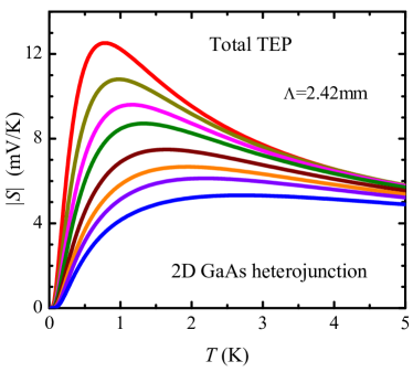
Figure 5: (Color online) Temperature dependencies of magnitude of total thermoelectric power $S\equiv S_{d}+S_{g}$ for various densities of electrons (from the top): $n_{s}=0.23$, $0.29$, $0.36$, $0.42$, $0.55$, $0.68$, $0.80$, and $1.06\times 10^{10}$ cm^-2.

IV Conclusions

Employing the energy expansion method to solve the Boltzmann equation and taking account of the screening of interactions in terms of finite-temperature STLS theory, we have carried out a theoretical investigation of the thermoelectric effect in a two-dimensional electron system with dilute electron density $0.23\leq n_{s}\leq 1.06\times 10^{10}$ cm^-2. The temperature dependencies of the diffusion and phonon-drag thermoelectric powers have been carefully analyzed for $T\leq 5$ K and our results exhibit deviations from the conventional simple power laws. We find that, in dilute 2D systems, $|S_{d}|/T$ remains constant only when $T\lesssim 0.1\varepsilon_{F}$ and it decreases with an increase of temperature out of this regime. We also observe a peak in the temperature dependence of $|S_{g}|$, which arises from competition between thermal broadening of distribution functions and decrease of the rate of nonequilibrium phonon production, induced by a temperature increase.

*

Appendix A Asymptotic behaviors of $S_{d}$ and $S_{g}$ in the high-electron-density limit

We verify that the energy-expansion method presented in section II produces the conventional expressions for $S_{d}$ and $S_{g}$ in the case $T\ll\varepsilon_{F}$ [$\varepsilon_{F}\equiv 2\pi n_{s}/(g_{s}m^{*})$ is the Fermi energy]. Obviously, in high-electron-density limit, it is sufficient to consider only the two lowest terms in the expansion of $g_{\bm{p}}$: $g_{\bm{p}}\approx[C_{0}\eta_{0}+C_{1}\eta_{1}(\varepsilon)]\cos\varphi_{\bm{p}}$. Based on the orthonormality conditions of $\eta_{n}(\varepsilon)$, Eq. (13), $\eta_{0}(\varepsilon)$ and $\eta_{1}(\varepsilon)$ can be written, respectively, as

$$\eta_{0}(\varepsilon) = \frac{1}{\sqrt{f_{0}(0)}}$$ (26)

$$= 1+\frac{1}{2}{\rm e}^{-\frac{\varepsilon_{F}}{T}}+\frac{3}{8}{\rm e}^{-\frac{2\varepsilon_{F}}{T}}+O\left({\rm e}^{-\frac{3\varepsilon_{F}}{T}}\right)$$

and

$$\eta_{1}(\varepsilon) = \frac{\sqrt{3}(\varepsilon_{F}-\varepsilon)}{\pi T}+\left\{\frac{3\sqrt{3}(\varepsilon_{F}-\varepsilon)}{2\pi^{3}T}\right.$$ (27)

$$\times\left.\left[\frac{1}{2}\left(\frac{\varepsilon_{F}}{T}\right)^{2}+\frac{\varepsilon_{F}}{T}+1\right]+\frac{\sqrt{3}}{\pi}\frac{\varepsilon_{F}}{T}\right\}{\rm e}^{-\frac{\varepsilon_{F}}{T}}$$

$$+O\left(T^{-5}{\rm e}^{-\frac{2\varepsilon_{F}}{T}}\right).$$

From Eqs. (26) and (27) it is obvious that the corrections to the leading terms of $\eta_{0,1}(\varepsilon)$ are exponentially small for $T\ll\varepsilon_{F}$ and hence $\eta_{0}(\varepsilon)=1$ and $\eta_{1}(\varepsilon)=\sqrt{3}(\varepsilon_{F}-\varepsilon)/(\pi T)$ can be used in the calculation that follows.

A.1 Temperature dependence of resistivity in the high-electron-density limit

Before proceeding to analyze $S_{d}$ and $S_{g}$ vs $T$, it is useful to evaluate the temperature dependence of resistivity, which is defined as $\rho=1/\sigma=m^{*}\left<\tau^{-1}\right>/(n_{s}e^{2})$ ($\left<\tau^{-1}\right>$ is the average inverse relaxation time) and is proportional to $Q_{00}$ in high-electron-density limit: $\rho=\eta_{0}^{3}Q_{00}/(g_{s}e^{2})=\eta_{0}^{3}(Q_{00}^{\rm imp}+Q_{00}^{\rm ph})/(g_{s}e^{2})$.

We first consider the temperature dependence of $Q_{00}^{\rm imp}$ resulting from RPA-screened electron-impurity interaction [$G(q)=0$ is used]. Using the potential given by Eq. (22), $Q_{00}^{\rm imp}$ can be expressed as

$$Q_{00}^{\rm imp}=\int d\varepsilon\delta(\varepsilon_{F}-\varepsilon)\Lambda^{\rm imp}(\varepsilon),$$ (28)

with $\Lambda^{\rm imp}(\varepsilon_{F})$ taking the form

$$\Lambda^{\rm imp}(\varepsilon_{F}) = \frac{1}{\varepsilon_{F}^{2}}\int_{0}^{2k_{F}}dq\left|\frac{U_{q}}{\epsilon(q,0)}\right|^{2}\frac{q^{2}}{\sqrt{4k_{F}^{2}-q^{2}}}.$$ (29)

In the low-temperature limit, $\Lambda^{\rm imp}(\varepsilon_{F})$ can be further expanded as

$$\Lambda^{\rm imp}(\varepsilon_{F}) = \frac{1}{\varepsilon_{F}^{2}}\int_{0}^{2k_{F}}dq\left|\frac{U_{q}}{\epsilon_{T=0}(q,0)}\right|^{2}\frac{q^{2}}{\sqrt{4k_{F}^{2}-q^{2}}}$$ (30)

$$+8\sqrt{\frac{T}{2\varepsilon_{F}^{3}}}|U_{2k_{F}}|^{2}\sum_{n=0}^{\infty}\left(\frac{m^{*}}{2\pi}\right)^{n}\frac{\left(\widetilde{V}_{2k_{F}}H_{2k_{F}}\right)^{n}}{[\epsilon_{T=0}(2k_{F},0)]^{n+2}}$$

$$\times(n+1)\left(\frac{4m^{*}T}{k_{F}^{2}}\right)^{n/2}\int_{0}^{\infty}\frac{dx}{\sqrt{x}}\phi(x),$$

with $\phi(x)=\int_{0}^{\infty}dy\frac{\sqrt{y}}{\cosh^{2}(y+x)}$.Gold and Dolgopolov (1986) From Eqs. (28) and (30) it follows that, for $T\ll\varepsilon_{F}$, $Q_{00}^{\rm imp}$ can be written as

$$Q_{00}^{\rm imp}=\Lambda^{\rm imp}(\varepsilon_{F})=\left.Q_{00}^{\rm imp}\right|_{T=0}+\Gamma^{\rm imp}(\varepsilon_{F})T+O(T^{3/2}),$$ (31)

with $\Gamma^{\rm imp}(\varepsilon_{F})$ determined by

$$\Gamma^{\rm imp}(\varepsilon_{F})=\frac{8{m^{*}}}{\pi\varepsilon_{F}^{2}}\frac{\widetilde{V}_{2k_{F}}H_{2k_{F}}}{[\epsilon_{T=0}(2k_{F},0)]^{3}}\int_{0}^{\infty}\frac{dx}{\sqrt{x}}\phi(x),$$ (32)

and $\left.Q_{00}^{\rm imp}\right|_{T=0}$ is obtained from Eq. (30) by setting $T=0$. From Eq. (31) it is clear that the first-order finite-temperature correction to $Q_{00}^{\rm imp}$ is linear in $T$, consistent with previous transport studies.Gold and Dolgopolov (1986); Das Sarma and Hwang (2004) Note that such a correction comes mainly from the temperature dependence of the dielectric function in the screened electron-impurity scattering potential. Moreover, if the screening of electron-impurity scattering is considered by means of the finite-temperature STLS theory, an additional temperature dependence associated with $G(q)$ needs to be taken into account.

Further, considering both the deformation and piezoelectric scatterings, we carry out the determination of the temperature dependence of $Q_{00}^{\rm ph}$ both in the BG ($T\ll T_{\rm BG}\ll\varepsilon_{F}$) and in the equipartition ($T_{\rm BG}\ll T\ll\varepsilon_{F}$) regimes. In both cases, $T_{\rm BG}\ll\varepsilon_{F}$ and hence we can make the approximation:

$$f_{0}(\varepsilon_{\bm{p}})[1-f_{0}(\varepsilon_{\bm{p}}+\Omega_{\bm{Q}\lambda})]\approx(1+n_{\bm{Q}\lambda})\Omega_{\bm{Q}\lambda}\delta(\varepsilon_{\bm{p}}-\varepsilon_{F}).$$ (33)

Performing the $\bm{p}$-integration in Eq. (18), $Q_{nn^{\prime}}^{\rm ph}$ for $n=n^{\prime}=0$ can be written as

$$Q_{00}^{\rm ph}=\int d\varepsilon\delta(\varepsilon_{F}-\varepsilon)\Lambda^{\rm ph}(\varepsilon)$$ (34)

with $\Lambda^{\rm ph}(\varepsilon)$ defined by ($k_{F}=\sqrt{2m^{*}\varepsilon_{F}}$)

$$\Lambda^{\rm ph}(\varepsilon_{F}) \approx \frac{1}{4\pi T\varepsilon_{F}^{2}}\sum_{\lambda,\pm}\int_{-\infty}^{\infty}|I(iq_{z})|^{2}dq_{z}\int_{0}^{\infty}qdq|M_{\bm{Q}\lambda}|^{2}$$ (35)

$$\times\Omega_{\bm{Q}\lambda}G_{\pm}(q,\Omega_{\bm{Q}\lambda})n_{\bm{Q}\lambda}(n_{\bm{Q}\lambda}+1).$$

Here, $G_{\pm}(q,\Omega_{\bm{Q}\lambda})\equiv 2(\varepsilon_{\bm{q}}\pm\Omega_{\bm{Q}\lambda})[(k_{F}q/m^{*})^{2}-(\Omega_{\bm{Q}\lambda}\pm\varepsilon_{\bm{q}})^{2}]^{-1/2}$ is associated with $\varphi_{\hat{\bm{p}\bm{q}}}$-integration over $\delta$ function.

In the BG regime, $T\ll T_{\rm BG}\ll\varepsilon_{F}$, $G_{\pm}(q,\Omega_{\bm{Q}\lambda})\approx 2m^{*}(\varepsilon_{q}\pm\Omega_{\bm{Q}\lambda})/(k_{F}q)$, $|I(iq_{z})|^{2}\rightarrow 1$, and $\epsilon(q,\Omega_{\bm{Q}\lambda})\approx q_{s}/q$ with $q_{s}=m^{*}e^{2}/(2\pi\varepsilon_{0}\kappa)$ as the screening wave vector. Thus, Eq. (35) can be rewritten in the low-temperature limit as

$$\Lambda^{\rm ph-BG}(\varepsilon_{F}) = \frac{T^{4}}{4\pi k_{F}\varepsilon_{F}^{2}}\sum_{\lambda}\frac{1}{u_{s\lambda}^{4}}\int_{-\infty}^{\infty}d\bar{q}_{z}$$ (36)

$$\times\int_{0}^{\infty}d\bar{q}|M_{\bm{Q}\lambda}|^{2}\frac{\bar{q}^{2}\bar{Q}{\rm e}^{\bar{Q}}}{\left({\rm e}^{\bar{Q}}-1\right)^{2}},$$

with $\bar{Q}=\sqrt{\bar{q}_{z}^{2}+\bar{q}^{2}}$. Substituting the explicit form of $M_{\bm{Q}\lambda}$ into Eq. (36), the contribution to $Q_{00}^{\rm ph}$ in the BG regime from the deformation potential, $Q_{00}^{\rm DP-BG}$, is given by

$$Q_{00}^{\rm DP-BG} = \frac{T^{5}\Xi^{2}}{8\pi dk_{F}\varepsilon_{F}^{2}u_{sl}^{6}}\int_{-\infty}^{\infty}d\bar{q}_{z}\int_{0}^{\infty}d\bar{q}\frac{\bar{q}^{2}\bar{Q}^{2}{\rm e}^{\bar{Q}}}{\left({\rm e}^{\bar{Q}}-1\right)^{2}}$$

$$= \frac{15\zeta(5)T^{5}\Xi^{2}}{2dk_{F}\varepsilon_{F}^{2}u_{sl}^{6}},$$

(37)

and the contribution from the screened piezoelectric interaction to $Q_{00}^{\rm ph-BG}$, $Q_{00}^{\rm PZ-BG}$, can be written as [$\bar{B}_{\rm LA}\equiv 9\bar{q}^{4}\bar{q}_{z}^{2}/\bar{Q}^{7}$ and $\bar{B}_{\rm TA}\equiv(\bar{q}^{6}+8\bar{q}^{2}\bar{q}_{z}^{4})/\bar{Q}^{7}$]

$$Q_{00}^{\rm PZ-BG} = \frac{\pi T^{5}e^{2}e_{14}^{2}}{\kappa^{2}dk_{F}\varepsilon_{F}^{2}q_{s}^{2}}\sum_{\lambda={\rm LA,TA}}\frac{1}{u_{{s}\lambda}^{6}}$$ (38)

$$\times\int_{-\infty}^{\infty}d\bar{q}_{z}\int_{0}^{\infty}d\bar{q}\frac{\bar{B}_{\lambda}\bar{q}^{4}\bar{Q}{\rm e}^{\bar{Q}}}{\left({\rm e}^{\bar{Q}}-1\right)^{2}}$$

$$= \frac{45\pi^{2}\zeta(5)T^{5}e^{2}e_{14}^{2}}{32\kappa^{2}dk_{F}\varepsilon_{F}^{2}q_{s}^{2}}\left(\frac{21}{u_{sl}^{6}}+\frac{29}{u_{st}^{6}}\right),$$

with $\zeta(x)$ as the Riemann function: $\zeta(5)\approx 1.037$. To derive Eq. (38), the $\varphi_{\bm{q}}$-independent forms of the scattering matrix are used: $|M_{\bm{Q}\lambda}|^{2}_{\rm piez}=4\pi^{2}e^{2}e_{14}^{2}B_{\lambda}/\left[\kappa^{2}du_{s\lambda}|\varepsilon(\bm{q},\Omega_{\bm{Q}\lambda})|^{2}\right]$ [$B_{\rm LA}\equiv 9q^{4}q_{z}^{2}/Q^{7}$ and $B_{\rm TA}\equiv(q^{6}+8q^{2}q_{z}^{4})/Q^{7}$],Lyo (1988) which differ slightly from those presented in Sec. III.

Using the material parameters for a GaAs/AlGaAs heterojunction, $Q_{00}^{\rm DP-BG}$ and $Q_{00}^{\rm PZ-BG}$ vary with temperature as $Q_{00}^{\rm DP-BG}\approx 1.936\times 10^{-5}T^{5}/n_{s}^{3/2}$ and $Q_{00}^{\rm PZ-BG}\approx 3.085\times 10^{-4}T^{5}/n_{s}^{3/2}$ ($n_{s}$ in $10^{11}$ cm^-2), respectively. This implies that, of the various electron-phonon scatterings, the (longitudinal-phonon) piezoelectric interaction is dominant at low temperature.

In the EP regime, $T_{\rm BG}\ll T\ll\varepsilon_{F}$ and $n_{\bm{Q}\lambda}\approx n_{\bm{Q}\lambda}+1\approx T/\Omega_{\bm{Q}\lambda}$, and Eq. (35) reduces to

$$\Lambda^{\rm ph-EP}(\varepsilon_{F}) \approx \frac{T}{4\pi k_{F}\varepsilon_{F}^{2}}\sum_{\lambda}\int_{-\infty}^{\infty}|I(iq_{z})|^{2}dq_{z}\int_{0}^{2k_{F}}dq$$ (39)

$$\times|M_{\bm{Q}\lambda}|^{2}\frac{q^{2}/\Omega_{\bm{q}\lambda}}{\sqrt{1-\frac{q^{2}}{4p^{2}}}}.$$

Accordingly, the contribution to $Q_{00}^{\rm ph-EP}$ from deformation and piezoelectric scatterings in the EP regime, $Q_{00}^{\rm DP-EP}$ and $Q_{00}^{\rm DP-EP}$, are given by

$$Q_{00}^{\rm DP-EP} = \frac{\Xi^{2}Tm^{*}}{2d\varepsilon_{F}u_{sl}^{2}}\int_{-\infty}^{\infty}|I(iq_{z})|^{2}dq_{z},$$ (40)

and

$$Q_{00}^{\rm PZ-EP} = \frac{32\pi Tm^{*}e^{2}e_{14}^{2}}{\kappa^{2}d\varepsilon_{F}k_{F}}\sum_{\lambda}\frac{1}{u_{s\lambda}^{2}}\int_{-\infty}^{\infty}|I(2ik_{F}\bar{q}_{z})|^{2}d\bar{q}_{z}$$ (41)

$$\times\int_{0}^{1}d\bar{q}\frac{\bar{q}^{2}\bar{B}_{\lambda}/\bar{Q}}{[1+q_{s}/(2k_{F}\bar{q})]^{2}\sqrt{1-\bar{q}^{2}}}.$$

Thus, we find that the electron-acoustic-phonon scattering tends to $\rho\sim Q_{00}^{\rm ph}\sim T^{5}$ in the BG regime and $\rho\sim Q_{00}^{\rm ph}\sim T$ in the EP regime.

It should be noted that the resistivity correction we found here in the analysis of electron-impurity scattering, which goes beyond the earlier “linear-in-$T$” result, is consistent with previous transport studies in Refs. Gold and Dolgopolov, 1986; Das Sarma and Hwang, 2004. In regard to electron-phonon scattering, our result concerning the power-law temperature dependence of resistivity due to piezoelectric scattering agrees with the previous one: in Refs. Price, 1984; Stormer et al., 1990 the contribution to inverse relaxation time due to piezoelectric scattering was found to be proportional to $T^{5}$. However, our deformation-scattering result is different from the $T^{7}$ law obtained previously. This is associated with the fact that the deformation scattering is taken to be unscreened in present paper, while a screened one was used in the previous studies.Price (1984); Stormer et al. (1990)

A.2 Diffusion thermoelectric power in the high-electron-density limit

To obtain the diffusion TEP $S_{d}$, one needs to consider the second term on the left hand side of Eq. (15). This term can be written for $n=0$ as

$$\frac{\nabla_{x}T}{T}\sum_{m}\alpha_{0m}\gamma_{m} = -\nabla_{x}T\left(1-\frac{\varepsilon_{F}}{T}\right){\rm e}^{-\frac{\varepsilon_{F}}{T}}$$

$$-\nabla_{x}T\frac{\varepsilon_{F}}{2T}{\rm e}^{-\frac{2\varepsilon_{F}}{T}}+O\left({\rm e}^{-\frac{3\varepsilon_{F}}{T}}\right),$$

and for $n=1$ we have

$$\frac{\nabla_{x}T}{T}\sum_{m}\alpha_{1m}\gamma_{m} = \frac{\sqrt{3}\pi}{3}\nabla_{x}T-\nabla_{x}T\frac{\sqrt{3}}{\pi}{\rm e}^{-\frac{\varepsilon_{F}}{T}}$$

$$\times\left[1+\frac{\varepsilon_{F}}{T}+\left(\frac{\varepsilon_{F}}{T}\right)^{2}\right]+O\left({\rm e}^{-\frac{2\varepsilon_{F}}{T}}\right).$$

It is clear that, in high-electron-density limit, the $n=0$ term is exponentially small while the term with $n=1$ is dominant and is given by

$$\frac{\nabla_{x}T}{T}\sum_{m}\alpha_{1m}\gamma_{m}\approx\frac{\sqrt{3}\pi}{3}\nabla_{x}T.$$ (44)

Assuming $\eta_{n}(\varepsilon_{\bm{p}})\approx\eta_{n}(\varepsilon_{\bm{p}-\bm{q}})$ in the case $T,T_{\rm BG}\ll\varepsilon_{F}$, $Q_{nn^{\prime}}^{\rm imp.ph}$ can be written as ($n,n^{\prime}\leq 1$)

$$Q_{nn^{\prime}}^{\rm imp,ph} = \int_{0}^{\infty}d\varepsilon\left[-\frac{\partial f_{0}(\varepsilon)}{\partial\varepsilon}\right]$$ (45)

$$\times\left[\frac{\sqrt{3}(\varepsilon_{F}-\varepsilon)}{\pi T}\right]^{n+n^{\prime}}\Lambda^{\rm imp,ph}(\varepsilon).$$

Using the low-temperature expansion of the Fermi functionLukyanov (1995)

$$f_{0}(\varepsilon)=\Theta(\varepsilon_{F}-\varepsilon)-\frac{\pi^{2}}{6}T^{2}\delta^{(1)}(\varepsilon-\varepsilon_{F})-\frac{7\pi^{4}}{30}T^{4}\delta^{(3)}(\varepsilon-\varepsilon_{F})+...$$ (46)

and performing the energy integration, the leading terms of $Q_{nn^{\prime}}^{\rm imp,ph}$ take the forms

$$Q_{10}^{\rm imp,ph}=Q_{01}^{\rm imp,ph}=-\frac{\sqrt{3}\pi T}{3}\frac{\partial\Lambda^{\rm imp,ph}(\varepsilon_{F})}{\partial\varepsilon_{F}},$$ (47)

and

$$Q_{11}^{\rm imp,ph}=Q_{00}^{\rm imp,ph}=\Lambda^{\rm imp,ph}(\varepsilon_{F}).$$ (48)

Substituting these $Q_{nn^{\prime}}$ terms into Eq. (15), the solution $C_{0}^{({\rm d})}$ can be written as

$$C_{0}^{({\rm d})}\approx\nabla_{x}T\frac{\pi^{2}}{3}T\frac{\partial}{\partial\varepsilon_{F}}\left[\Lambda^{\rm imp}(\varepsilon_{F})+\Lambda^{\rm ph}(\varepsilon_{F})\right]^{-1},$$ (49)

and the diffusion TEP takes the form

$$S_{d} \approx -\frac{\pi^{2}T}{3e}\left.\Lambda^{\rm imp}(\varepsilon_{F})\right|_{T=0}\frac{\partial}{\partial\varepsilon_{F}}\frac{1}{\left.\Lambda^{\rm imp}(\varepsilon_{F})\right|_{T=0}}$$ (50)

$$+\frac{\pi^{2}T}{3e}\frac{\partial}{\partial\varepsilon_{F}}\left[\frac{\Gamma(\varepsilon_{F})T+\Lambda^{\rm ph}(\varepsilon_{F})}{\left.\Lambda^{\rm imp}(\varepsilon_{F})\right|_{T=0}}\right].$$

From Eq. (50) we see that the first term on the right hand side agrees with the well-known Mott formula.Mott and Davis (1979) Considering the fact that $Q_{00}$ relates to $n_{s}$ approximately as $Q_{00}\approx m^{*}\left<\tau^{-1}\right>/(g_{s}n_{s})$ and ignoring the energy-dependence of $\left<\tau^{-1}\right>$, $S_{d}\approx\pi^{2}T/(3e\varepsilon_{F})$ can be obtained. However, if one assumes $\left<\tau^{-1}\right>\sim\varepsilon_{F}^{p}$, we obtain $S_{d}\approx\pi^{2}T/(3e\varepsilon_{F})(1+p)$, in agreement with the results of Refs.Karavolas et al., 1990; Karavolas and Butcher, 1991.

In Eq. (50), the second term on the right hand side is a low-temperature correction to the leading term and it is proportional to $T^{2}$. Obviously, in the BG regime, this correction comes only from the temperature dependence of the screening of electron-impurity scattering, since the phonon contribution is proportional to $T^{6}$ in BG regime [$\Lambda^{\rm ph}(\varepsilon_{F})\sim T^{5}$] and it can be ignored. However, in the equipartition regime, the electron-phonon scattering results in $\Lambda^{\rm ph}(\varepsilon_{F})$ being linear in $T$. Hence, both the electron-impurity and electron-phonon scatterings lead to a deviation of $S_{d}$ vs $T$ from the linear rule when $T_{\rm BG}\ll T\ll\varepsilon_{F}$.

A.3 Phonon-drag thermoelectric power in the high-electron-density limit

To investigate the phonon-drag effect in thermoelectric power, one needs to study the driving term $D_{n}$ in Eq. (15). Performing substitution, $\bm{q}\rightarrow-\bm{q}$ for $+$ term and $\bm{p}\rightarrow\bm{p}+\bm{q}$ for $-$ term, Eq. (16) can be rewritten as

$$D_{n} = 2\pi\sum_{{\bm{Q}},{\bm{p}},\lambda}|\widetilde{M}_{{\bm{Q}}\lambda}|^{2}\delta(\varepsilon_{{\bm{p}}+{\bm{q}}}-\varepsilon_{{\bm{p}}}-\Omega_{{\bm{Q}}\lambda})\tau_{{\rm p}\lambda}u^{x}_{\bm{Q}\lambda}$$ (51)

$$\times\frac{\Omega_{\bm{Q}\lambda}}{T}n_{{\bm{Q}}\lambda}(1+n_{{\bm{Q}}\lambda})\left[f_{0}(\varepsilon_{\bm{p}})-f_{0}(\varepsilon_{{\bm{p}}+{\bm{q}}})\right]$$

$$\times\left[\chi_{n}(\bm{p}+\bm{q})-\chi_{n}(\bm{p})\right].$$

Considering only the driving term $D_{n}$ with $n=0,1$, the solution of Eq. (15), $C_{0}^{(\rm g)}$, can be written as

$$C_{0}^{(\rm g)} = \frac{\nabla_{x}T}{T}\frac{Q_{11}D_{0}-Q_{01}D_{1}}{Q_{11}Q_{00}-Q_{01}Q_{10}}$$ (52)

$$\approx \frac{\nabla_{x}T}{T}\left(\frac{1}{Q_{00}}D_{0}-\frac{Q_{01}}{Q_{00}Q_{11}}D_{1}\right).$$

Using Eqs. (47) and (48), the phonon-drag $S_{g}$ is determined by

$$S_{g}=-\frac{1}{eT}\left[D_{0}+\frac{\sqrt{3}}{3}\pi TD_{1}\frac{\partial}{\partial\varepsilon_{F}}\ln\Lambda(\varepsilon_{F})\right].$$ (53)

Recognizing that $\chi_{n}(\bm{p}+\bm{q})-\chi_{n}(\bm{p})\approx 4\pi q\cos\varphi_{\bm{q}}\eta_{n}(\varepsilon_{\bm{p}})/p^{2}$ in the case $T\ll\varepsilon_{F}$, $S_{g}$ finally takes the form

$$S_{g} = -\frac{2\pi^{2}}{m^{*}eT}\frac{\partial\ln\Lambda(\varepsilon_{F})}{\partial\varepsilon_{F}}\sum_{{\bm{Q}},{\bm{p}},\lambda}|\widetilde{M}_{{\bm{Q}}\lambda}|^{2}\delta(\varepsilon_{{\bm{p}}+{\bm{q}}}-\varepsilon_{{\bm{p}}}-\Omega_{{\bm{Q}}\lambda})$$ (54)

$$\times\tau_{{\rm p}\lambda}u_{\bm{Q}\lambda}\frac{q^{2}\Omega_{\bm{Q}\lambda}}{QT}n_{{\bm{Q}}\lambda}(1+n_{{\bm{Q}}\lambda})\left[f_{0}(\varepsilon_{\bm{p}})-f_{0}(\varepsilon_{{\bm{p}}+{\bm{q}}})\right].$$

Note that this expression for $S_{g}$ reduces to the one widely used in literatureCantrell and Butcher (1987a); Khveshchenko and Reizer (1997); Fletcher (2002) if $\frac{\partial\ln\Lambda(\varepsilon_{F})}{\partial\varepsilon_{F}}$ is replaced by $1/\varepsilon_{F}$.

To further analyze the power law of $S_{g}$ vs $T$ in the high-$n_{s}$ limit, one has to study the temperature dependence of $\tau_{{\rm p}\lambda}$. At sufficiently low temperature, it is reasonable to assume that boundary scattering dominates phonon relaxation and the mean free path of phonons, $\Lambda$, is independent of $T$. Under this consideration, $S_{g}$ in the BG regime, $S_{g}^{\rm BG}$, can be written as

$$S_{g}^{\rm BG} \approx -\frac{{m^{*}}^{2}T^{3}}{4\pi^{2}k_{F}n_{s}e}\sum_{\lambda}\int_{-\infty}^{\infty}d\bar{q}_{z}\int_{0}^{\infty}d\bar{q}$$ (55)

$$\times\left|M_{\bm{Q}\lambda}\right|^{2}\frac{\tau_{{\rm p}\lambda}\bar{q}^{2}\bar{Q}{\rm e}^{\bar{Q}}}{u_{s\lambda}^{2}({\rm e}^{\bar{Q}}-1)^{2}},$$

and, in the EP regime, it takes the form

$$S_{g}^{\rm EP} \approx -\frac{{m^{*}}^{2}}{4\pi^{2}k_{F}n_{s}e}\sum_{\lambda}\tau_{{\rm p}\lambda}u_{s\lambda}\int_{-\infty}^{\infty}dq_{z}|I(iq_{z})|^{2}\int_{0}^{\infty}dq$$ (56)

$$\times\left|M_{\bm{Q}\lambda}\right|^{2}\frac{q^{2}}{Q\sqrt{1-\left(\frac{m^{*}}{pq}\right)^{2}\left(\Omega_{\bm{Q}\lambda}-\varepsilon_{\bm{q}}\right)^{2}}}.$$

$S_{g}^{\rm BG}$ can be further simplified by substituting explicit forms of the deformation and piezoelectric scattering matrices into it and then performing momentum integration:

$$S^{\rm BG}_{g} \approx -\frac{15{m^{*}}^{2}\Xi^{2}T^{4}\tau_{\rm p,LA}\zeta(5)}{2\pi\sqrt{2\pi}dn_{s}^{3/2}eu_{sl}^{4}}$$ (57)

$$-\frac{45{m^{*}}^{2}ee_{14}^{2}T^{4}\zeta(5)}{32\pi\sqrt{2\pi}d\kappa^{2}q_{s}^{2}n_{s}^{3/2}}\left(21\frac{\tau_{\rm p,LA}}{u_{sl}^{4}}+29\frac{\tau_{\rm p,TA}}{u_{st}^{4}}\right).$$

From Eqs.(55) and (56) we see that, when $T\rightarrow 0$, the phonon-drag thermoelectric power tends to zero as $T^{4}$ in the BG regime and it reaches a saturation value in the EP regime. Note that such behavior of $S_{g}$ vs $T$ in the BG regime has already been demonstrated in Refs.Tieke et al., 1998; Khveshchenko and Reizer, 1997, while, as far as we know, the temperature-independence of $S_{g}$ in the EP regime, obtained here, is a new prediction.

References

- Wang and Li (2008a) L. Wang and B. Li, Physics World 21(2), 27 (2008a).
- Bauer et al. (2010) G. E. Bauer, A. H. MacDonald, and S. Maekawa, Solid State Commun. 150, 459 (2010).
- Segal (2008a) D. Segal, Phys. Rev. Lett. 100, 105901 (2008a).
- Hu et al. (2006) B. Hu, L. Yang, and Y. Zhang, Phys. Rev. Lett. 97, 124302 (2006).
- Li et al. (2005) B. Li, J. H. Lan, and L. Wang, Phys. Rev. Lett. 95, 104302 (2005).
- Segal and Nitzan (2005) D. Segal and A. Nitzan, Phys. Rev. Lett. 94, 034301 (2005).
- Li et al. (2004) B. Li, L. Wang, and G. Casati, Phys. Rev. Lett. 93, 184301 (2004).
- Terraneo et al. (2002) M. Terraneo, M. Peyrard, and G. Casati, Phys. Rev. Lett. 88, 094302 (2002).
- Lo et al. (2008) W. C. Lo, L. Wang, and B. Li, J. Phys. Soc. Jpn 77, 054402 (2008).
- Segal (2008b) D. Segal, Phys. Rev. E 77, 021103 (2008b).
- Li et al. (2006) B. Li, L. Wang, and G. Casati, Appl. Phys. Lett. 88, 143501 (2006).
- Wang and Li (2008b) L. Wang and B. Li, Phys. Rev. Lett. 101, 267203 (2008b).
- Uchida et al. (2008) K. Uchida, S. Takahashi, K. Harii, J. Ieda, W. Koshibae, K. Ando, S. Maekawa, and E. Saitoh, Nature 455, 778 (2008).
- Uchida et al. (2010) K. Uchida, J. Xiao, H. Adachi, J. Ohe, S. Takahashi, J. Ieda, T. Ota, Y. Kajiwara, H. Umezawa, H. Kawai, G. E. W. Bauer, S. Maekawa, and E. Saitoh, Nature Materials 9, 894 (2010).
- Jaworski et al. (2010) C. M. Jaworski, J. Yang, S. Mack, D. D. Awschalom, J. P. Heremans, and R. C. Myers, Nature Materials 9, 898 (2010).
- Johnson (2010) M. Johnson, Solid State Commun. 150, 543 (2010).
- Seebeck (1823) T. J. Seebeck, Repts. Prussian Acad. Sci. (1823).
- Seebeck (1825) T. J. Seebeck, Abhandlungen der Deutschen Akademie der Wissenshaften zu Berlin , p.265 (1825).
- Frederikse (1953) H. Frederikse, Phys. Rev. 92, 248 (1953).
- Geballe and Hull (1954) T. Geballe and G. Hull, Phys. Rev. 94, 1134 (1954).
- Geballe and Hull (1955) T. Geballe and G. Hull, Phys. Rev. 98, 940 (1955).
- Obloh et al. (1984) H. Obloh, K. Vonklitzing, and K. Ploog, Surf. Sci. 142, 236 (1984).
- Nicholas et al. (1984) R. J. Nicholas, T. H. H. Vuong, M. A. Brummell, J. C. Portal, and M. Razeghi, in Proceedings of the 17th International Conference on Physics of Semiconductors (1984) p. 389.
- Fletcher et al. (1985) R. Fletcher, J. C. Maan, and G. Weimann, Phys. Rev. B 32, 8477 (1985).
- Davidson et al. (1986) J. S. Davidson, E. D. Dahlberg, A. J. Valois, and G. Y. Robinson, Phys. Rev. B 33, 2941 (1986).
- Fletcher et al. (1986) R. Fletcher, J. C. Maan, K. Ploog, and G. Weimann, Phys. Rev. B 33, 7122 (1986).
- Obloh et al. (1986) H. Obloh, K. Vonklitzing, K. Ploog, and G. Weimann, Surf. Sci. 170, 292 (1986).
- Ruf et al. (1988) C. Ruf, H. Obloh, B. Junge, E. Gmelin, K. Ploog, and G. Weimann, Phys. Rev. B 37, 6377 (1988).
- Fletcher et al. (1988) R. Fletcher, M. D’Iorio, A. S. Sachrajda, R. Stoner, C. T. Foxon, and J. J. Harris, Phys. Rev. B 37, 3137 (1988).
- Ying et al. (1994) X. Ying, V. Bayot, M. B. Santos, and M. Shayegan, Phys. Rev. B 50, 4969 (1994).
- Fletcher et al. (1994) R. Fletcher, J. J. Harris, C. T. Foxon, M. Tsaousidou, and P. N. Butcher, Phys. Rev. B 50, 14991 (1994).
- Bayot et al. (1995) V. Bayot, E. Grivei, H. C. Manoharan, X. Ying, and M. Shayegan, Phys. Rev. B 52, R8621 (1995).
- Tieke et al. (1996) B. Tieke, U. Zeitler, R. Fletcher, S. A. J. Wiegers, A. K. Geim, J. C. Maan, and M. Henini, Phys. Rev. Lett. 76, 3630 (1996).
- Fletcher et al. (1997) R. Fletcher, V. M. Pudalov, Y. Feng, M. Tsaousidou, and P. N. Butcher, Phys. Rev. B 56, 12422 (1997).
- Miele et al. (1998) A. Miele, R. Fletcher, E. Zaremba, Y. Feng, C. T. Foxon, and J. J. Harris, Phys. Rev. B 58, 13181 (1998).
- Fletcher et al. (1998) R. Fletcher, V. M. Pudalov, and S. Cao, Phys. Rev. B 57, 7174 (1998).
- Fletcher (2002) R. Fletcher, Physica E 12, 478 (2002).
- Maximov et al. (2004) S. Maximov, M. Gbordzoe, H. Buhmann, L. W. Molenkamp, and D. Reuter, Phys. Rev. B 70, 121308 (2004).
- Zhang et al. (2004) J. Zhang, S. K. Lyo, R. R. Du, J. A. Simmons, and J. L. Reno, Phys. Rev. Lett. 92, 156802 (2004).
- Rafael et al. (2004) C. Rafael, R. Fletcher, P. T. Coleridge, Y. Feng, and Z. R. Wasilewski, Semicond. Sci. Technol. 19, 1291 (2004).
- Chickering et al. (2009) W. E. Chickering, J. P. Eisenstein, and J. L. Reno, Phys. Rev. Lett. 103, 046807 (2009).
- Chickering et al. (2010) W. E. Chickering, J. P. Eisenstein, L. N. Pfeiffer, and K. W. West, Phys. Rev. B 81, 245319 (2010).
- Girvin and Jonson (1982) S. M. Girvin and M. Jonson, J. Phys. C 15, L1147 (1982).
- Zawadzki and Lassnig (1984) W. Zawadzki and R. Lassnig, Surf. Sci. 142, 225 (1984).
- Nicholas (1985) R. J. Nicholas, J. Phys. C 18, L695 (1985).
- Cantrell and Butcher (1987a) D. G. Cantrell and P. N. Butcher, J. Phys. C 20, 1993 (1987a).
- Cantrell and Butcher (1987b) D. G. Cantrell and P. N. Butcher, J. Phys. C 20, 1985 (1987b).
- Kubakaddi et al. (1987) S. S. Kubakaddi, B. G. Mulimani, and V. M. Jali, Phys. Status Solidi B 139, 267 (1987).
- Kundu et al. (1987) S. Kundu, C. K. Sarkar, and P. K. Basu, J. Appl. Phys. 61, 5080 (1987).
- Lyo (1988) S. K. Lyo, Phys. Rev. B 38, 6345 (1988).
- Basak and Kar (1989) S. Basak and R. Kar, Semicond. Sci. Technol. 91, 1142 (1989).
- Kubakaddi et al. (1989) S. S. Kubakaddi, P. N. Butcher, and B. G. Mulimani, Phys. Rev. B 40, 1377 (1989).
- Okuyama and Tokuda (1990) Y. Okuyama and N. Tokuda, Phys. Rev. B 42, 7078 (1990).
- Karavolas et al. (1990) V. K. Karavolas, M. J. Smith, T. M. Fromhold, P. N. Butcher, B. G. Mulimani, B. L. Gallagher, and J. P. Oxley, J. Phys.: Condens. Matter 2, 10401 (1990).
- Karavolas and Butcher (1991) V. C. Karavolas and P. N. Butcher, J. Phys.: Condens. Matter 3, 2597 (1991).
- X. L. Lei (1994) X. L. Lei, J. Phys.: Condens. Matter 6, L305 (1994).
- Zianni et al. (1994) X. Zianni, P. N. Butcher, and M. J. Kearney, Phys. Rev. B 49, 7520 (1994).
- Khveshchenko (1996) D. V. Khveshchenko, Phys. Rev. B 54, R14317 (1996).
- Wu et al. (1996) M. W. Wu, N. J. M. Horing, and H. L. Cui, Phys. Rev. B 54, 5438 (1996).
- Cooper et al. (1997) N. R. Cooper, B. I. Halperin, and I. M. Ruzin, Phys. Rev. B 55, 2344 (1997).
- Khveshchenko and Reizer (1997) D. V. Khveshchenko and M. Y. Reizer, Phys. Rev. Lett. 78, 3531 (1997).
- Tsaousidou et al. (1999) M. Tsaousidou, P. N. Butcher, and S. S. Kubakaddi, Phys. Rev. Lett. 83, 4820 (1999).
- Karavolas and Triberis (2001) V. C. Karavolas and G. P. Triberis, Phys. Rev. B 65, 033307 (2001).
- Kundu and Datta (2001) S. Kundu and R. Datta, Phys. Status Solidi A 186, 471 (2001).
- Tsaousidou et al. (2001) M. Tsaousidou, P. N. Butcher, and G. P. Triberis, Phys. Rev. B 64, 165304 (2001).
- Sankeshwar et al. (2005) N. S. Sankeshwar, M. D. Kamatagi, and B. G. Mulimani, Phys. Status Solidi B 242, 2892 (2005).
- Sergeev et al. (2005) A. Sergeev, M. Y. Reizer, and V. Mitin, Phys. Rev. Lett. 94, 136602 (2005).
- Zhou et al. (2010) X. Zhou, B. A. Piot, M. Bonin, L. W. Engel, S. Das Sarma, G. Gervais, L. N. Pfeiffer, and K. W. West, Phys. Rev. Lett. 104, 216801 (2010).
- Lilly et al. (2003) M. P. Lilly, J. L. Reno, J. A. Simmons, I. B. Spielman, J. P. Eisenstein, L. N. Pfeiffer, K. W. West, E. H. Hwang, and S. Das Sarma, Phys. Rev. Lett. 90, 056806 (2003).
- Spivak et al. (2010) B. Spivak, S. A. Kivelson, and X. P. A. Gao, Rev. Mod. Phys. 82, 1743 (2010).
- Singwi et al. (1968) K. Singwi, M. Tosi, R. Land, and A. Sjölander, Phys. Rev. 176, 589 (1968).
- Schweng and B hm (1994) H. K. Schweng and H. M. B hm, Z. Phys. B 95, 481 (1994).
- Das Sarma and Hwang (2004) S. Das Sarma and E. H. Hwang, Phys. Rev. B 69, 195305 (2004).
- Das Sarma and Hwang (2003) S. Das Sarma and E. H. Hwang, Phys. Rev. B 68, 195315 (2003).
- Das Sarma and Hwang (1999) S. Das Sarma and E. H. Hwang, Phys. Rev. Lett. 83, 164 (1999).
- Herring (1954) C. Herring, Phys. Rev. 95, 954 (1954).
- Callaway (1991) J. Callaway, Quantum Theory of the Solid State, 2nd ed. (Academic, San Diego, 1991).
- Allen (1978) P. B. Allen, Phys. Rev. B 17, 3725 (1978).
- Jonson (1976) M. Jonson, J. Phys. C 9, 3055 (1976).
- Lei et al. (1985) X. L. Lei, J. L. Birman, and C. S. Ting, J. Appl. Phys. 58, 2272 (1985).
- Bardeen and Shockley (1950) J. Bardeen and W. Shockley, Phys. Rev. 80, 72 (1950).
- Gold and Dolgopolov (1986) A. Gold and V. T. Dolgopolov, Phys. Rev. B 33, 1076 (1986).
- Price (1984) P. Price, Solid State Commun. 51, 607 (1984).
- Stormer et al. (1990) H. L. Stormer, L. N. Pfeiffer, K. W. Baldwin, and K. W. West, Phys. Rev. B 41, 1278 (1990).
- Lukyanov (1995) V. K. Lukyanov, J. Phys. G: Nucl. Part. Phys. 21, 145 (1995).
- Mott and Davis (1979) N. Mott and E. Davis, Electronic processes in non-crystalline materials (Oxford, Clarendon, 1979).
- Tieke et al. (1998) B. Tieke, R. Fletcher, U. Zeitler, M. Henini, and J. C. Maan, Phys. Rev. B 58, 2017 (1998).