Spiky development at the interface in Rayleigh-Taylor instability: Layzer approximation with second harmonic

Abstract

Layzer’s approximation method for investigation of two fluid interface structures associated with Rayleigh Taylor instability for arbitrary Atwood number is extended with the inclusion of second harmonic mode leaving out the zeroth harmonic one. The modification makes the fluid velocities vanish at infinity and leads to avoidance of the need to make the unphysical assumption of the existence of a time dependent source at infinity.

The present analysis shows that for an initial interface perturbation with curvature exceeding $1/(2\sqrt{A})$, where $A$ is the Atwood number there occurs an almost free fall of the spike with continuously increasing sharpening as it falls. The curvature at the tip of the spike also increases with Atwood number. Certain initial condition may also result in occurrence of finite time singularity as found in case of conformal mapping technique used earlier. However bubble growth rate is not appreciably affected.

Hydrodynamic instabilities such as Rayleigh Taylor instability(RTI) which sets in when a lighter fluid supports a heavier fluid against gravity or Richtmyer Meshkov instability(RMI) which is initiated when a shock passes an interface between two fluids with different acoustic impedances are of increasing importance in a wide range of physical phenomena starting from inertial confinement fusion (ICF) to astrophysical ones like supernova explosions. In ICF, the capsule shell undergoes the RTI both in the acceleration and deceleration phases. RTI can retard the formation of the hot spot by the cold RTI spike of capsule shell resulting in the destruction of the ignition hot spot or autoignition${\cite[cite]{[\@@bibref{}{lin04}{}{}]}-\cite[cite]{[\@@bibref{}{at04}{}{}]}}$. The hydrodynamic instabilities lead to development of heavy fluid ’spikes’ penetrating into the lighter fluid and ’bubbles’ of lighter fluid rising through the heavier fluid. Different approaches have been used for the study of such problems. Among these Layzer’s[5] approach applied to single mode potential flow model${\cite[cite]{[\@@bibref{}{jh94}{}{}]}-\cite[cite]{[\@@bibref{}{ss03}{}{}]}}$ is a useful one giving approximate estimate of both Rayleigh Taylor and Richtmyer Meshkov instability evolution. The bubbles were shown by Zhang[7] to rise at a rate tending asymptotically to a terminally constant velocity while spikes were shown to descend with a constant acceleration. However, whether for bubbles or for the spikes, Zhang’s analysis was applicable only for Atwood number $A=1$, i.e, only for fluid-vacuum interface. An extension to arbitrary value of Atwood number $A$ was done by Goncharov[8]. Within limitations of Layzer’s model as pointed out by Mikaelian[12] bubbles were shown to rise with a velocity tending to an asymptotic value dependent on $A$ and having a fairly close agreement with the simulation results of Ramaprabhu et al.[13]. But the spikes were found to descend with a terminal constant velocity in contrast to a constant acceleration as obtained by Zhang[7] for $A=1$.

Asymptotic spike evolution in Rayleigh Taylor instability behaving almost as a free fall was obtained by Clavin and Williams[14] and also by Duchemin et al.[15] by conformal mapping method. Associated with the free fall of the spike, the surface curvature of the spike was also found to increase with time (i.e the spike sharpens as it falls).

In the single mode Layzer model with generalization [8] for arbitrary Atwood number the equation to the interface taken in X-Y plane as

$$y\equiv\eta(x,t)=\eta_{0}(t)+\eta_{2}(t)x^{2};$$ (1)

with $\eta_{0}(t)>0$, $\eta_{2}(t)<0$ for bubble while $\eta_{0}(t)<0$, $\eta_{2}(t)>0$ for spike. The velocity potential describing the motion of the heavier fluid (density $\rho_{h}$) and the lighter fluid (density $\rho_{l}$) are ( gravity $g$ is along the negative $y$ direction)

$$\phi_{h}(x,y,t)=a(t)\cos{(kx)}e^{-k(y-\eta_{0}(t))};\quad y>0\quad(heavierfluid)$$ (2)

$$\phi_{l}(x,y,t)=b_{0}(t)y+b_{1}(t)\cos{(kx)}e^{k(y-\eta_{0}(t))};\quad y<0\quad(lighterfluid)$$ (3)

where $k$ is the wave number and $a(t),b_{0}(t),b_{1}(t)$ are amplitudes.This conventional single mode Layzer model has the drawback that rather than conforming to the physical requirement: $v_{ly}\rightarrow 0$ as $y\rightarrow-\infty$ it necessitates the assumption of a time dependent source at $y\rightarrow-\infty$[16]. To avoid this difficulty we modify the single mode Layzer model by replacing the zeroth mode term $b_{0}(t)y$ in Eq.(3) by a second harmonic term viz,

$$\phi_{l}(x,y,t)=b_{1}(t)\cos{(kx)}e^{k(y-\eta_{0}(t))}+b_{2}(t)\cos{(2kx)}e^{2k(y-\eta_{0}(t))};\quad y<0$$ (4)

Eqs.(2) and (4) give

$$v_{hy}(y\rightarrow\infty)=-\frac{\partial\phi_{h}}{\partial y}]_{y\rightarrow\infty}=0$$ (5)

$$v_{ly}(y\rightarrow-\infty)=-\frac{\partial\phi_{l}}{\partial y}]_{y\rightarrow-\infty}=0$$ (6)

The kinematic boundary conditions at the interface (1) are

$$\frac{\partial\eta}{\partial t}+v_{hx}\frac{\partial\eta}{\partial x}=v_{hy}$$ (7)

$$\frac{\partial\eta}{\partial x}(v_{hx}-v_{lx})=v_{hy}-v_{ly}$$ (8)

Setting the pressure boundary condition $p_{h}=p_{l}$ in Bernoulli’s equation for the heavier and lighter fluids leads to${\cite[cite]{[\@@bibref{}{qz98}{}{}]}\cite[cite]{[\@@bibref{}{vg02}{}{}]}\cite[cite]{[\@@bibref{}{ss03}{}{}]}\cite[cite]{[\@@bibref{}{ss07}{}{}]}-\cite[cite]{[\@@bibref{}{rb11}{}{}]}}$

$$\rho_{h}[-\frac{\partial\phi_{h}}{\partial t}+\frac{1}{2}(\vec{\nabla}\phi_{h})^{2}+g\eta]-\rho_{l}[-\frac{\partial\phi_{l}}{\partial t}+\frac{1}{2}(\vec{\nabla}\phi_{l})^{2}+g\eta]=f_{h}(t)-f_{l}(t)$$ (9)

Following the usual procedure${\cite[cite]{[\@@bibref{}{mrg09}{}{}]}-\cite[cite]{[\@@bibref{}{rb11}{}{}]}}$ ,i.e, expanding $\eta(x,t)$ and the velocity potentials in powers of $(kx)$ and equating coefficients of $(kx)^{r},(r=0,2)$ we obtain from Eqs.(7)-(9) the evolution equation for the RT bubbles/spikes (nondimensionalized) tip elevation $\xi_{1}=k\eta_{0}$, curvature $\xi_{2}=\eta_{2}/k$ and velocity $\xi_{3}=k^{2}a/\sqrt{kg}$

$$\frac{d\xi_{1}}{d\tau}=\xi_{3}$$ (10)

$$\frac{d\xi_{2}}{d\tau}=-(3\xi_{2}+\frac{1}{2})\xi_{3}$$ (11)

$$\frac{d\xi_{3}}{d\tau}=-\frac{[2\xi_{2}(\xi_{2}-\frac{1}{2})^{2}+\xi_{3}^{2}(\xi_{2}-\alpha)(\xi_{2}-\beta)]}{[2(\xi_{2}-\frac{1}{2})(\xi_{2}^{2}-\frac{1}{4}\frac{r+1}{r-1})]}$$ (12)

where

$$\alpha,\beta=\frac{(r+4)\pm\sqrt{12r+13}}{2(r-1)};r=\frac{\rho_{h}}{\rho_{l}}$$ (13)

and

$$\tau=t\sqrt{kg}$$ (14)

is nondimensionalized time.

Starting from a set of initial values $\xi_{1}>0$, $\xi_{2}<0$ and $\xi_{3}>0$ which correspond to the description of temporal evolution of the tip of the bubble we arrive at the asymptotic value ($\tau\rightarrow\infty$)

$$\xi_{2}\rightarrow-\frac{1}{6}$$ (15)

and

$$[\xi_{3}]_{asymp}=\sqrt{\frac{8A}{3(5A+3)}}>[\xi_{3}]_{asymp}^{classical}=\sqrt{\frac{2}{3}\frac{A}{1+A}}$$ (16)

(by classical we mean the single mode Layzer approximation as used by Goncharov[8]). Two values coincide as $A(=\frac{\rho_{h}-\rho_{l}}{\rho_{h}+\rho_{l}})\rightarrow 1$. The growth rate of the development of the height of the bubble tip is shown in Figure 1 and compared with classical value. It is seen that presence or absence of a source does not give rise to any qualitatively significant change in the growth rate of the bubble height[8][9][17].

To get spike like behavior of the perturbation of the interface we used

$$\xi_{1}<0,\quad\xi_{2}>0\quad and\quad\xi_{3}<0$$ (17)

Corresponding to a start from an initial value

$$[\xi_{2}]_{initial}>\frac{1}{2}\sqrt{\frac{r+1}{r-1}},\quad[\xi_{3}]_{initial}<0$$ (18)

Eq.(11) shows that $\xi_{2}$ increases monotonically ($\frac{d\xi_{2}}{d\tau}>0$ for all $\tau>0$) while from Eq.(12) it follows that the depth of the spike tip below the surface of separation increases continuously ($\frac{d\xi_{1}}{d\tau}=\xi_{3}<0$ and $\frac{d\xi_{3}}{d\tau}<0$). These are shown in Figures 2(a) and 2(b) by plotting $\xi_{2}(\tau)$ and $\xi_{3}(\tau)$ as function of $\tau$ obtained from numerical solution of Eqs.(11) and (12) by employing fifth order Runge-Kutta-Fehlberg method. The initial value taken are $[\xi_{2}]_{initial}=1.0$ and $[\xi_{3}]_{initial}=-0.5$ which satisfy condition (17) for all the following three values of $r=2(A=\frac{1}{3})$, $r=5(A=\frac{2}{3})$, $r=20(A=\frac{19}{21})$. The value of $\xi_{2}$ which represents the curvature at the tip of the spike is an increasing function of $\tau$ for every value of the Atwood number $A$ (Figure 2(a)). Moreover for every given value of $\tau$ the curvature $\xi_{2}$ increases with $A$. This implies that the spike continues to sharpen with time as well as with increasing Atwood number and is explicitly shown in Figure 3. Figure 2(b) shows that except very close to the starting instant the spike descends with a constant acceleration $\simeq-g$ (i.e, nearly a free fall). This agrees with the conclusions[7] for Atwood number $A=1$.

The time development of spiky behavior for $[\xi_{2}]_{initial}>\frac{1}{2}\sqrt{\frac{r+1}{r-1}}$ and $[\xi_{3}]_{initial}<0$ is demonstrated in Figures4(a) and 4(b). This is shown both for increasing $A$ with fixed $\tau$ (Figure 4(a)) and with increasing $\tau$ for given $A$ (Figure 4(b)). But for $\frac{1}{2}<[\xi_{2}]_{initial}<\frac{1}{2}\sqrt{\frac{r+1}{r-1}}$ with $[\xi_{3}]_{initial}<0$ one encounters development of finite time singularity i.e, $\xi_{2}\rightarrow\infty$ and $\xi_{3}\rightarrow-\infty$ at a finite value of $\tau$. The possibility of the occurrence of such an eventuality at (or near) the tip of the spike is also found to arise when the RT instability is addressed by conformal mapping method${\cite[cite]{[\@@bibref{}{tb03}{}{}]}-\cite[cite]{[\@@bibref{}{tn93}{}{}]}}$ as mentioned by Clavin and Williams[14].

Finally for a trajectory starting from $(\xi_{3})_{initial}<0$ and $0<(\xi_{2})_{initial}<\frac{1}{2}\sqrt{\frac{r+1}{r-1}}=\frac{1}{2}\sqrt{\frac{1}{A}}$ one finds that $\xi_{2}$ continues to increase towards $\xi_{2}=\frac{1}{2}$, i.e, the spike continues to sharpen as time progresses and its speed of fall slowly decreases in magnitude. Because of the presence of singularity at $\xi_{2}=\frac{1}{2}$(Eq.(12)), it is not possible to continue the numerical integration towards and beyond this point. This is shown in Figure 5 for initial values in the domain mentioned above.

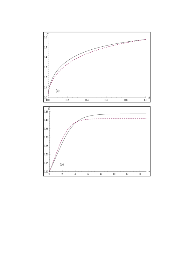
Figure 1: (a).Variation of $\xi_{3}$ against $A$ and (b).Variation of $\xi_{3}$ against $\tau$, where the black line gives the saturation growth rate since by Eqs.(11) and (12)and the dashed line gives the classical value of growth rate of the tip of the bubble.

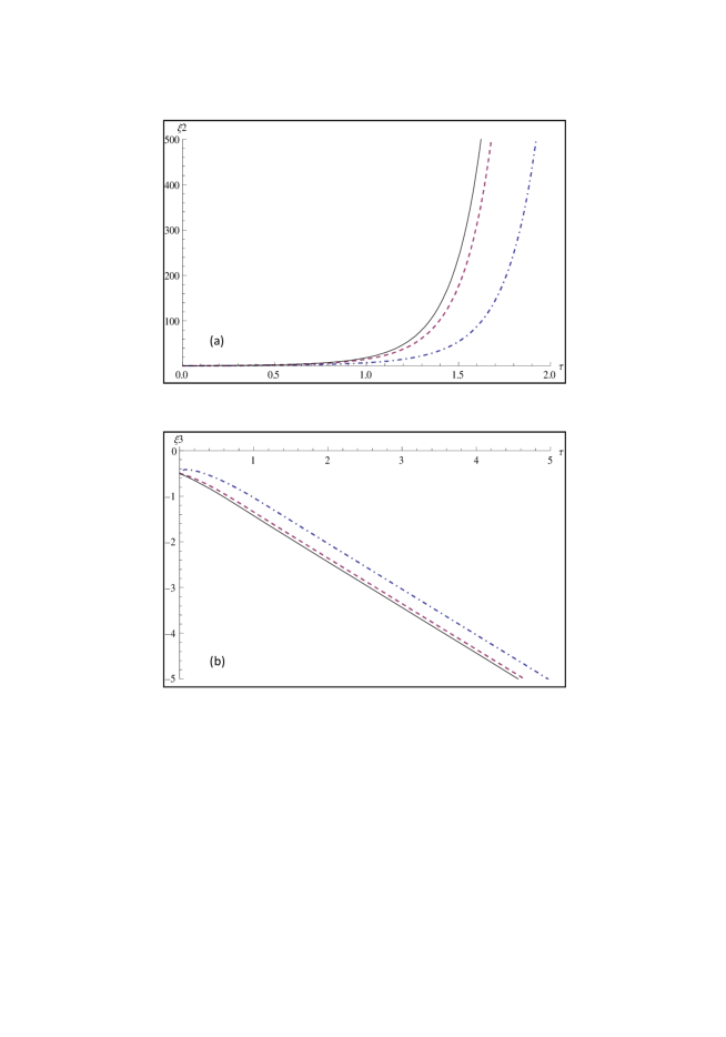
Figure 2: (a) Variation of $\xi_{2}$ against $\tau$ and (b) Variation of $\xi_{3}$ against $\tau$ with initial value $\xi_{1}=-0.1,\xi_{2}=1.0,\xi_{3}=-0.5$ and $r$=2(dot-dashed), 5(dashed), 20(black).

Figure 3: Variation of $\xi_{2}$ against $A$ with initial value $\xi_{1}=-0.1,\xi_{2}=1.0,\xi_{3}=-0.5$.

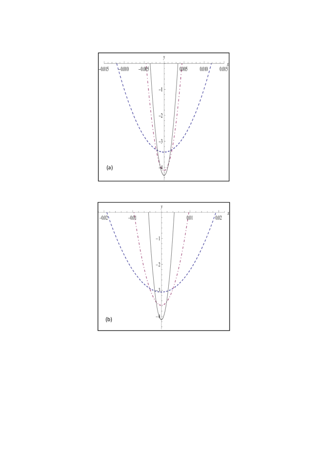
Figure 4: Shows formation of spikes for different values of (a)$A$ = $\frac{1}{3}$(dashed), $\frac{2}{3}$(dot-dashed), $\frac{19}{21}$(black) for fixed $\tau$= 2.5 and (b)$\tau$ = 2.1(Dashed), 2.3(dot-dashed), 2.5(black) for fixed $A$ = $\frac{2}{3}$.

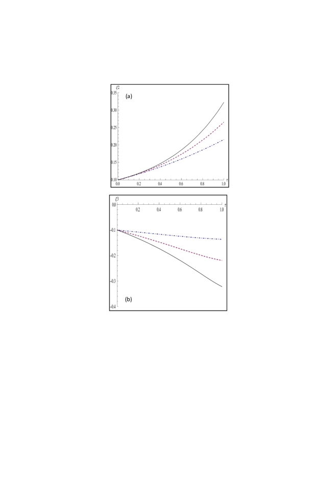
Figure 5: (a) Variation of $\xi_{2}$ against $\tau$ and (b) Variation of $\xi_{3}$ against $\tau$ with initial value $\xi_{1}=-0.1,\xi_{2}=0.1,\xi_{3}=-0.1$ and $r$=2(dot-dashed), 5(dashed), 20(black).

References

- [1] J.D.Lindl,P.Amendt, R.L.Berger et al. Phys. Plasmas 11, 339 (2004).
- [2] D. Batani,W.Nazakov,T.Hall,T.Lower,M.Koenig,B.Faral,A.B.Mounaix,N.Grandjouan Phys. Rev. E 62, 8573 (2000).
- [3] R. Dezulian,F.Canova,S.Barbanotti, et al. Phys. Rev. E 73, 047401 (2006).
- [4] S. Atzeni, J. Meyer-ter-vehn The Physics of Inertial Fusion: Beam Plasma Interaction, Hydrodynamics, Hot Dense Mater (Oxford University, London,2004).
- [5] D. Layzer Astrophys. J. 122, 1 (1955).
- [6] J. Hecht, U. Alon, and D. Shvarts Phys. Fluids 6, 4019 (1994).
- [7] Q. Zhang Phys. Rev. Lett. 81, 3391 (1998).
- [8] V.N.Goncharov Phys. Rev. Lett. 88, 134502 (2002).
- [9] Sung-Ik-Sohn, Q. Zhang Phys. Fluids 13, 3493 (2001).
- [10] Sung-Ik-Sohn, J. Comput. App. Math. 177, 367 (2005).
- [11] Sung-Ik-Sohn, Phys. Rev. E 67, 026301 (2003).
- [12] K.O. Mikaelian Phys. Rev. E 78, 015303(R) (2008).
- [13] P. Ramaprabhu, G. Dimonte, Yuan-Nan Young, A.C. Calder, B. Fryxell Phys. Rev. E 74, 066308 (2006).
- [14] P.Clavin, F. Williams J. Fluid Mech. 525, 105 (2005).
- [15] L. Duchemin, C. Josserand, P. Clavin Phys. Rev. Lett. 94, 224501 (2005).
- [16] S.I. Abarzhi, K. Nishihara, J. Glimm Phys. Lett. A 317, 470 (2003).
- [17] Sung-Ik-Sohn, Phys. Rev. E 75, 066312 (2007).
- [18] Sung-Ik-Sohn, Phys. Rev. E 80, 055302(R) (2009).
- [19] M.R.Gupta, S.Roy, M.Khan, H.C.Pant, S.Sarkar, M.K. Srivastava Phys. Plasmas 16, 032303 (2009).
- [20] R.Betti, J.Sanz, Phys. Rev. Lett. 97, 205002 (2006).
- [21] M.R.Gupta, L.Mandal, S.Roy, M.Khan Phys. Plasmas 17, 012306 (2010).
- [22] R. Banerjee, L.Mandal, S.Roy, M.Khan,M.R.Gupta Phys. Plasmas 18, 022109 (2011).
- [23] T. Yoshikawa,A. Balk Math. Comput. Modelling 38, 113 (2003).
- [24] S. Tanveer Proc. R. Soc. Lond. A 441,501 (1993).