The intergalactic medium over the last 10 billion years II: Metal-line absorption and physical conditions

Abstract

We investigate the metallicity evolution and metal content of the intergalactic medium (IGM) and galactic halo gas from $z=2\rightarrow 0$ using 110-million particle cosmological hydrodynamic simulations. We focus on the detectability and physical properties of UV resonance metal-line absorbers observable with Hubble’s Cosmic Origins Spectrograph (COS). We confirm that galactic superwind outflows are required to enrich the IGM to observed levels down to $z=0$ using three wind prescriptions contrasted to a no-wind simulation. Our favoured momentum-conserved wind prescription deposits metals closer to galaxies owing to its moderate energy input, while the more energetic constant wind model enriches the warm-hot IGM (WHIM) 6.4 times more. Despite these significant differences, all wind models produce metal-line statistics within a factor of two of existing observations. This is because O vi, C iv, Si iv, and Ne viii absorbers primarily arise from $T<10^{5}$ K, photo-ionised gas that is enriched to similar levels in the three feedback schemes. O vi absorbers trace the diffuse phase with $\rho/\bar{\rho}\la 100$, which is enriched to $\sim 1/50\;{\rm Z}_{\odot}$ at $z=0$, although the absorbers themselves usually exceed $0.3\;{\rm Z}_{\odot}$ and arise from inhomogeneously distributed, un-mixed winds. Turbulent broadening is required to match the observed equivalent width and column density statistics for O vi. C iv and Si iv absorbers trace primarily $T\sim 10^{4}$ K gas inside haloes ($\rho/\bar{\rho}\ga 100$), although there appear to be too many C iv absorbers relative to observations. We predict COS will observe a population of Ne viii photo-ionised absorbers tracing $T<10^{5}$ K, $\rho/\bar{\rho}\sim 10$ gas with equivalent widths of 10-20 mÅ. Mg x and Si xii are rarely detected in COS S/N=30 simulated sight lines ($dn/dz\ll 1$), although simulated Si xii detections trace halo gas at $T=10^{6-7}$ K. In general, the IGM is enriched in an outside-in manner, where wind-blown metals released at higher redshift reach lower overdensities, resulting in higher ionisation species tracing lower-density, older metals. At $z=0$, the 90% of baryons outside of galaxies are enriched to $\bar{Z}=0.096\;{\rm Z}_{\odot}$, but the 65% of unbound baryons in the IGM have $\bar{Z}=0.018\;{\rm Z}_{\odot}$ and contain only 4% of all metals, a large decline from 20% at $z=2$, because metals from early winds often re-accrete onto galaxies while later winds are less likely to escape their haloes. We emphasise that our results are sensitive to how metal mixing is treated in the simulations, and argue that the lack of mixing in our scheme may be the largest difference with other similar publications.

1 Introduction

The intergalactic medium (IGM) contains the majority of the Universe’s baryons. The best available IGM tracer is the intervening ${\rm Ly}\alpha$ absorption forest observed in quasar spectra (, 1998). Contributing a lesser but still significant amount of absorption are intervening metal lines that trace the enrichment history of the IGM (e.g. , 1987, 1995, 1996, 2001, 2003, 2004, 2008, 2008). Since metal absorption is often found far from the sites of star formation, analytic models and simulations strongly suggest that metals must be transported out from galaxies into the IGM via large-scale galactic outflows (e.g. Tegmark, Silk, & Evrard, 1993; Nath & Trentham, 1997; , 2001, 2003b, 2006, 2006, 2007, 2008, 2009a; Tornatore et al., 2010; , 2011; Tescari et al., 2011).

The observation and interpretation of IGM metal-line absorbers provides critical insights into the physics of galaxy formation. First, galactic outflows that enrich the IGM concurrently regulate the growth of galaxies by removing gas from star-forming regions. Second, the census of IGM metals provides a unique and independent constraint on the integrated amount of star formation in our Universe; indeed, the metal census within galaxies falls significantly short of the expectations from cosmic star formation, which is known as the “missing metals problem” (e.g. , 2004, 2007). Finally, the amount and physical state of the metals in the IGM alters how gas cools (e.g. , 1993, 2007, 2009b), thereby impacting the efficiency by which galaxies receive gas from the IGM (e.g. , 1996, 2005, 2010). Hence studying IGM metal absorbers provides unique insights into the cycle of baryons between galaxies and their surrounding gas.

Despite the importance of IGM metal absorbers, the chasm between observations and a theory of metal lines remains wide. Many basic questions concerning IGM chemical enrichment remain poorly understood. Answering such questions is now becoming feasible owing to the recent installation of the Cosmic Origins Spectrograph (COS) on the Hubble Space Telescope (HST), whose central mission is to improve our knowledge of the low-redshift IGM. Key questions include:

$\bullet$ What is the metallicity of the IGM? At redshifts of $z=2-3$ measurements range between $10^{-3.5}-10^{-2.0}\;{\rm Z}_{\odot}$ (, 1996, 1998, 2003, 2004), while by $z=0$ a value of $0.1\;{\rm Z}_{\odot}$ is typically quoted (, 2001, 2001, 2003). While this suggests an increasing metallicity with time, the interpretation is complicated by an evolution in how metals trace the IGM baryon distribution. Owing to cosmic expansion, a given column density H i system traces a higher overdensity at lower redshifts (, 1999); a similar trend, modulated by evolving photo-ionisation rates, also exists for metals. One consequence of these effects is that summing the column densities of metal lines to find an integrated ion density ($\Omega_{\rm ion}$) does not necessarily translate into a global metallicity ($\Omega_{\rm metal}$). (2006) argued that the non-trivial ionisation correction from C iv to total carbon abundance evolved with redshift, resulting in a relatively flat $\Omega_{\hbox{C\,{\sc iv}}}$ that masks a significant increase in the metallicity of the IGM. These measurements have now been made down to $z\sim 0$ (e.g. , 2008, 2010), and COS should provide significantly more insights into the relationship between metallicity and density over most of cosmic time.

$\bullet$ What temperature is the enriched IGM gas? High-ionisation lines commonly observed in the IGM such as C iv and O vi can arise both from photo-ionisation and collisional ionisation. The low densities and hard quasar-dominated metagalactic flux can produce such high ionisation states, as can hotter gas in the warm-hot intergalactic medium (WHIM) of gas shock-heated during large-scale structure formation. There is vigorous debate as to whether observed high-ionisation lines trace collisionally-ionised hot metals at $T>10^{5}\,$K (e.g. , 2006, 2008; Cen & Chisari, 2011; , 2011; Tepper-Garcia et al., 2011) or low-density photo-ionised gas at $T<10^{5}\,$K (e.g. , 2008b, 2008, 2009, hereafter OD09). The increased sensitivity of COS enables multiple ions to be detected in many systems, allowing independent constraints on the nature of high-ionisation systems.

$\bullet$ How homogeneously are metals distributed in the IGM? If metals are well-mixed throughout the IGM, metal lines will cool more baryons, possibly leading to increased gas accretion onto galaxies and hence an increase in star formation (, 2009a). If metals are poorly mixed as observations suggest (, 2006, 2007), then a census of O vi cannot straightforwardly be converted to a census of baryons (e.g. , 2000, 2005) since O vi only traces the baryons in over-enriched regions (OD09; Tepper-Garcia et al., 2011). The analysis of observed metal-line systems often yields inconclusive answers, with complex absorbers suggesting multi-phase gas components (e.g. , 2004, 2005, 2006, 2008; Howk et al., 2009; Narayanan et al., 2009). The higher signal-to-noise provided by COS will be critical for disentangling these effects.

A number of reasons exist for our less complete knowledge of metal absorbers compared to that of the ${\rm Ly}\alpha$ forest. Observationally, metal lines are weaker and, therefore, harder to detect. Moreover, many key ionisation states are buried within the ${\rm Ly}\alpha$ forest or occur at X-ray wavelengths where current sensitivities are limited (e.g. , 2003; Nicastro et al., 2005; , 2006; Fang et al., 2010). Theoretically, IGM enrichment depends sensitively on the transport mechanism out of galaxies, which is poorly constrained, while the ${\rm Ly}\alpha$ forest is less affected (Kollmeier et al. 2003; OD09; Davé et al., 2010; Tescari et al., 2011). Furthermore, converting metal ions into metallicities typically requires a detailed knowledge of the photo-ionisation rates at energies poorly constrained by the data or, if collisionally ionised, is highly sensitive to gas temperatures (e.g. , 2002) and hence detailed cooling rates (e.g. , 2007). However, there are many more metal transitions observable compared to hydrogen transitions, providing an opportunity to synthesise a wider suite of observations into a single coherent framework to determine the physical state of IGM metals. Hydrodynamic simulations that evolve the metallicity and ionisation state of the IGM self-consistently along with the enriching galaxy population offer a way to develop such a framework within a modern hierarchical context.

In this paper, we employ state-of-the-art cosmological hydrodynamic simulations to study the $z=0-2$ IGM as traced by high ionisation metal lines. Our strategy involves examining what can be learned by observations targeting quasar absorption line spectra randomly sampling the IGM, which represents a volume-weighted measure. We focus on high ionisation lines including O vi, C iv, Si iv, Ne viii, Mg x, and Si xii. Low ionisation lines (e.g. C ii, Si ii, Mg ii) are not addressed as they trace higher density gas where self-shielding renders the assumption of a uniform ionisation background insufficient. We briefly comment on N v and O v predictions. This paper directly follows Davé et al. (2010, Paper I in this series, hereafter D10), which discussed the ${\rm Ly}\alpha$ forest and the physical conditions of baryons in the IGM. The next paper in this series will study correlations between galaxies and absorbers (Kollmeier et al. in prep., Paper III).

While we will show predictions for observable quantities with COS, we do not intend these to be used for direct comparisons with data. We are more interested in showing how plausible variations in the physics manifest themselves in forefront observations, particularly in terms of answering some of the questions outlined above. For instance, we will discuss how integrated column densities trace the underlying IGM metallicity, how various ions observable with COS trace the temperature and density of the enriched IGM baryons, and how absorber alignment statistics can constrain the homogeneity of metals in the IGM. We will do all this for several prescriptions of galactic outflows, to better understand how COS observations can constrain this important physical process of galaxy formation.

A description of our cosmological hydrodynamic simulations and our artificial spectra follows in §2. §3 concentrates on the evolving physical conditions of metals, subdivided by phase between $z=2\rightarrow 0$. We simulate COS metal-line absorber observations in §4 and relate them to their physical conditions in §5, demonstrating that only a fraction of IGM metals are probed via UV resonance absorption lines. We spend §6 exploring physically plausible model variations both to demonstrate the inherent uncertainties in interpreting metal-line observations and to distill what can be learned using relatively straight-forward statistics in a sample size similar to the one that COS will observe. §7 discusses the successes and failures of our simulations and compares them to simulations by other groups. We conclude in §8. For readers who want a briefer overview of the results, we suggest first reading the conclusions section and following the sections listed after each of the main findings for more detail.

2 Methods and Simulations

We utilise our modified version (, 2008) of the Gadget-2 N-body + Smoothed Particle Hydrodynamic (SPH) code (, 2005) to evolve a series of cosmological simulations to $z=0$. The details of the simulations can be found in §2 of D10; they have also been used and described in (2010). Briefly, our cosmology agrees with the WMAP-7 constraints (Jarosik et al., 2011) and uses the following values: $\Omega_{\rm M}=0.28$, $\Omega_{\rm\Lambda}=0.72$, $h\equiv H_{0}/(100\;{\rm km}\,{\rm s}^{-1}{\rm Mpc}^{-1})=0.7$, a primordial power spectrum index $n=0.96$, an amplitude of the mass fluctuations scaled to $\sigma_{8}=0.82$, and $\Omega_{\rm b}=0.046$.

2.1 Wind Implementations

We briefly recap the implementations of galactic winds in these simulations; for a more extensive description see (2008). The basic technical implementation is the one described in (2003a) and incorporated into Gadget-2. In a given timestep, a particle in a star-forming region has $p_{ej}=\eta\times{\rm SFR}/m_{\rm p}$ of being ejected, where $\eta$ is the mass-loading factor, SFR the star-formation rate, and $m_{\rm p}$ the particle mass. The ejection velocity, ${v_{\rm wind}}$, is oriented according to ${\bf v}\times\nabla\Phi$, where ${\bf v}$ is the particle velocity and $\nabla\Phi$ is the gradient of the gravitational potential, resulting in winds propagating perpendicular to galactic disks. To allow the particle to escape the ISM of its host, hydrodynamic forces are turned off until one of two criteria are met: either $1.95\times 10^{10}\;{\rm km}\,{\rm s}^{-1}/{v_{\rm wind}}$ years have passed or (more often) the particle flows out to a density of less than 10% of the star formation critical density.

In our constant wind (cw) model, we employ an ejection velocity of ${v_{\rm wind}}=680\;{\rm km}\,{\rm s}^{-1}$ and a mass loading factor of $\eta=2$ for all galaxies. The slow wind model has ${v_{\rm wind}}=340\;{\rm km}\,{\rm s}^{-1}$ and $\eta=2$. Both of these wind models are similar to (2003a), except for their assumed velocity; they use ${v_{\rm wind}}=484\;{\rm km}\,{\rm s}^{-1}$. The momentum-conserved wind model, inspired by the (2005) models of radiation pressure-driven winds, has ${v_{\rm wind}}=3\sigma\sqrt{f_{\rm L}-1}$ where $f_{\rm L}$ is the luminosity in units of the Eddington luminosity required to expel gas from a galaxy potential, and $\eta=\sigma_{0}/\sigma$ where $\sigma_{0}=150\;{\rm km}\,{\rm s}^{-1}$ and $\sigma$ is the galaxy’s internal velocity dispersion calculated by a group finder run during the evolution of the simulation (see , 2008).

The metallicity of an ejected wind particle is the metallicity of the SPH particle at the time of ejection. SPH particles are continually self-enriched while they are eligible for star formation. In this scheme, both ejected winds and newly formed stars have the metallicity of the SPH particle at the time of the ejection or formation event; wind particles are essentially ejected ISM SPH particles. Note that only particles above the critical star-formation density threshold are eligible to form stars or to become launched as a wind. Cooling, which is never suppressed, invariably allows the launched winds to cool and maintain a temperature of $\sim 10^{4}$ K while decoupled. Once the hydrodynamic forces are restored, which always occurs deep inside haloes given the two criteria listed above, the SPH particle interacts normally. In practice, re-coupled wind particles show a bimodal behaviour: (i) they shock heat to temperatures above the peak cooling efficiencies for metal-enriched gas ($T\sim 10^{5}-10^{6}$ K), or (ii) they shock heat to a lower temperature where metal-line cooling is efficient and then rapidly cool to $T\sim 10^{4}$ K. The most important determining factor appears to be ${v_{\rm wind}}$, which we will show when we consider IGM enrichment patterns among the different wind models in §3.

2.2 Simulations

Our naming convention for our simulations continues the precedent we established in our recent papers: r[boxsize]n[number of particles per side][wind model], where the initial letter “r” indicates the particular choice of cosmology above. The main simulations that we explore are evolved in a cubic periodic volume that is $48h^{-1}{\rm Mpc}$ on a side: r48n384nw (nw: no winds), r48n384cw (cw: constant winds), r48n384sw (sw: slow winds), and r48n384vzw (vzw: momentum-conserved winds). These simulations were also used in (2010), D10, and Davé et al. (2011a, b). The main simulations are listed in Table 1. The gas and dark matter particle masses are $3.56\times 10^{7}M_{\odot}$ and $1.81\times 10^{8}M_{\odot}$, respectively.

Table 1: Simulations

Namea	$L^{b}$	$N_{\rm side}^{c}$	${v_{\rm wind}}^{d}$	$\eta^{e}$	$E_{\rm wind}/E_{\rm SN}^{f}$	$Z$ Coolingg	$f_{\tau}^{h}$	$\Omega_{*}/\Omega_{b}(z=0)^{i}$
r48n384nw	48	384	–	–	0.0	CIE	0.9	0.213
r48n384cw	48	384	680	2	0.96	CIE	0.9	0.045
r48n384sw	48	384	340	2	0.24	CIE	0.8	0.124
r48n384vzw	48	384	$\propto\sigma$	$\propto\sigma^{-1}$	0.45-0.56	CIE	0.67	0.097
r16n128cw	16	128	680	2	0.96	CIE	0.9	0.040
r16n128cw-PI	16	128	680	2	0.96	PI	0.9	0.037
r16n128vzw	16	128	$\propto\sigma$	$\propto\sigma^{-1}$	0.41-0.54	CIE	0.67	0.096
r16n128vzw-PI	16	128	$\propto\sigma$	$\propto\sigma^{-1}$	0.41-0.56	PI	0.67	0.088

^aSuffix: nw- no-wind, cw- constant wind, sw- slow wind, vzw- momentum-conserved winds.

^bBox length of cubic volume, in comoving $h^{-1}{\rm Mpc}$.

^cNumber of dark matter and SPH particles per box side.

^dWind velocity in $\;{\rm km}\,{\rm s}^{-1}$.

^eMass loading, where $\dot{M}_{\rm wind}=\eta\dot{M}_{*}$.

^fWind energy divided by total SNe energy assuming $E_{\rm SN}=9.7\times 10^{48}{\rm erg}/\;{\rm M}_{\odot}$. Range of values at $z=$0,1,2,3 for vzw.

^gMetal-line cooling. CIE- Collisional Ionising Equilibrium cooling rates, PI- Photo-ionisation-dependent cooling rates.

^hFactor ${\rm Ly}\alpha$ optical depth is scaled in determining ionisation background normalisation.

ⁱFraction of baryons in stars at $z=0$.

Four other simulations listed in Table 1 are evolved in a $16h^{-1}{\rm Mpc}$ box with $2\times 128^{3}$ particles, the same resolution as the main simulations. We use these to test the effects of metal-line cooling with photo-ionisation on metal-line observations, because Tepper-Garcia et al. (2011) and (2011) demonstrate that this could significantly alter observations of O vi versus using collisionally ionised metal-line cooling rates. Despite their smaller volume, we will demonstrate in §6.2 that these simulations’ results remain converged compared to the 48 $h^{-1}{\rm Mpc}$ simulations, likely because absorbers are mainly associated with sub-$M^{*}$ galaxies that are sufficiently sampled in both size volumes. We add the suffix PI to those simulation names evolved using the photo-ionised cooling rates of (2009b).

2.3 Spectra

Spectra are generated as described in §2.3 of D10. Briefly, 70 continuous lines of sight are created from $z=2\rightarrow 0$ for each model using our spectral generation code specexbin (, 2006). We generate mock spectra using only the strongest transition for an ion (e.g. the 1031.93Å line for O vi, the 1548.19Å line for C iv) and convolve the spectra with the COS line spread function (LSF). We add Gaussian random noise with a signal to noise ratio S/N=30 per 6 $\;{\rm km}\,{\rm s}^{-1}$ pixel to simulate the highest quality data obtainable using COS. We employ the continuum provided directly by the simulation, and do not attempt to mimic the observational procedure of fitting a continuum, since at low redshifts the sparseness of absorption features usually results in a robust and reliable continuum fit.

We fit absorbers in the spectra using AutoVP (, 1997), obtaining a column density $N$, line width $b$, and redshift $z$ for each absorber. We consider each metal transition separately and do not combine them into a single spectrum with all the transitions. This assumes that, in observations, each transition can be reliably identified and fit without contamination from other lines, which is typically true at low redshifts.

2.4 Ionisation Background

The metagalactic flux amplitude is adjusted to match the observed evolution of the ${\rm Ly}\alpha$ forest mean flux decrement. We multiply the ${\rm Ly}\alpha$ optical depth by the same values of $f_{\tau}$ that we calculated in D10 and presented in Table 1 of that paper. In practice, we renormalise our CLOUDY (Ferland et al., 1998, version 08.00) ionisation tables so that the magnitude of the ionisation background is multiplied by $1/f_{\tau}$, which effectively shifts the ionisation fractions of all ions by $1/f_{\tau}$ in density under the assumption of an optically thin gas. The vzw normalised (2001, HM2001) $z=0.2$ background (i.e. $J_{\nu}$ multiplied by $1.5$) is shown in Figure 1 in black. Three other backgrounds are also displayed, which will be described in §6.1 when we explore the effects of variations in the ionisation background.

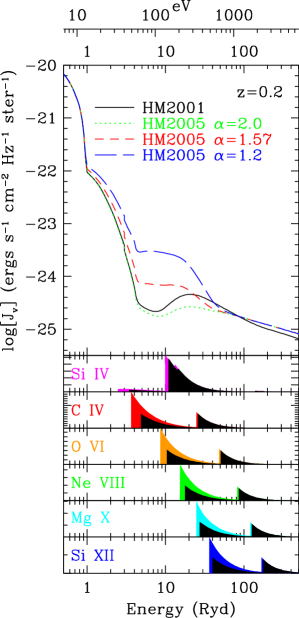
Figure 1: The ionisation background spectra explored in this paper. HM2001 is the (2001) spectrum multiplied by 1.5 to match the observed ${\rm Ly}\alpha$ flux decrement (D10). Three other backgrounds generated using CUBA (, 2001) with varying slopes for quasar spectra above the Lyman limit are also displayed (HM2005). Energies are listed in units of Rydbergs as well as electron volts (eV, top x-axis). Below are photo-ionisation cross-sections for various ions. Coloured regions show the magnitude of the cross-section from the ionisation state below to the specified ionisation state, while black regions show the cross-section from the specified state to the state above. For these panels, levels of $10^{-18}{\rm cm}^{2}$ are indicated by large ticks on the $y$-axis and $10^{-19}{\rm cm}^{2}$ are indicated by small ticks, with the $y$-axis starting at zero in all cases.

We also display the photo-ionisation cross-sections of various ions used in CLOUDY (Verner & Yakovlev, 1995; Verner et al., 1996) on a linear scale in the bottom panels of Figure 1. The coloured regions show the ionisation cross-section of the next lowest ionisation state to the specified ionisation state, while the black shading indicates the cross-section from that state to the next highest state. For example, the magenta shading indicates the cross-section for Si iii to Si iv, and the black shading indicates the cross-section for Si iv to Si v. With the exception of Si iv, all cases shown are lithium-like ions and display a trend of increasing ionisation energy and declining cross-section with higher atomic number. Metal ion cross-sections are complex, which is exemplified by the Si iii and Si iv cross-sections peaking above 10 Ryd even though Si iii has the lowest ionisation energy (2.5 Ryd) of all the species we consider. The multiple offset wedges, two in the case of lithium-like ions, correspond to different subshells in the ground state.

2.5 Chemodynamical Model

We follow the production of four heavy elements (C, O, Si, & Fe) from three sources: Type II Supernovae (SNe), Type Ia SNe, and AGB stars as explained in (2008). The details of the enrichment scheme are in §2.1 of D10. Cosmic oxygen and silicon production is dominated by Type II SNe, while carbon production is augmented significantly by AGB stars but still primarily arises from SNe (, 2008). We do not follow neon and magnesium directly when generating Ne viii and Mg x statistics but instead use oxygen as their proxy, which is a reasonable approximation given that all three elements arise primarily from Type II SNe. The resulting abundances are [Ne/O]=0.16 and [Mg/O]=-0.21 for (2004) SNe yields when using (2005) solar abundances, which we scale to throughout this paper whenever quoting metallicities. We assume the same Type II SNe origin for nitrogen by using [N/O]=-0.40, but note that this does not include secondary nitrogen production in AGB stars, which is likely significant. The solar metal mass fraction by weight, $\;{\rm Z}_{\odot}$, is 0.0122 and the mass fractions of carbon, nitrogen, oxygen, neon, magnesium, and silicon are 0.00218, 0.00062, 0.00541, 0.00103, 0.00061, and 0.00067 respectively. We also do not consider depletion of these elements onto dust grains, although recent results suggest that there may be dust in the IGM (Ménard et al., 2010; Zu et al., 2011) that contains as much as 50% of the mass of intergalactic metals.

3 Metal Physical Conditions

3.1 Density-Temperature Phase Space

The density-temperature phase space diagrams of metals residing in the IGM are displayed in the left panels of Figure 2 for our preferred vzw model at $z=2$, 1, and 0. The diagrams are coloured by metallicity while the brightness indicates the fraction of baryons. On the right side are depicted the $z=0$ phase space diagrams for the other three wind models. Histograms along the x- and y-axes depict the relative fraction of metal mass at a given density and temperature, respectively.

The metals populate the cosmic phase diagram differently than the baryons (see e.g. D10) with the density and temperature dependence of metallicity linked to the type of outflows that put them there, which we will discuss in §3.2. Here we focus on generic trends seen among all the wind models, contrasting them with the no-wind case.

Following D10, we divide the gas component into four phases, demarcated by the solid lines in the figures:

• Diffuse ($T<T_{\rm th},\delta<\delta_{\rm th}$),

• WHIM ($T>T_{\rm th},\delta<\delta_{\rm th}$),

• Hot halo ($T>T_{\rm th},\delta>\delta_{\rm th}$),

• Condensed ($T<T_{\rm th},\delta>\delta_{\rm th}$),

where $T_{\rm th}=10^{5}$ K represents the division between the “cool” and “hot” phases, and $\delta_{\rm th}$ represents the division between bound (halo) gas and unbound (IGM) gas. These definitions are designed to provide a physically-motivated demarcation between cosmic baryon phases. $T_{\rm th}=10^{5}$ K is near the peak in the helium and metal cooling curve that causes a minimum in the temperature distribution of baryons, while the density threshold separates truly intergalactic baryons, i.e. those not associated with gravitationally collapsed structures, from baryons that lie predominantly within the virial radii of galaxy halos. Following (1996), we set

$$\delta_{\rm th}=6\pi^{2}(1+0.4093(1/f_{\Omega}-1)^{0.9052})-1,\\$$ (1)

where

$$f_{\Omega}=\frac{\Omega_{m}(1+z)^{3}}{\Omega_{m}(1+z)^{3}+(1-\Omega_{m}-\Omega_{\Lambda})(1+z)^{2}+\Omega_{\Lambda}}.$$ (2)

$\delta_{\rm th}$ evolves from a value of $\approx 60$ at high redshift to $\approx 120$ by $z=0$. As in D10, we adopt Equation 1 to be 1/3rd the (1996) mean enclosed density, which corresponds to the density at $r_{200}$ for objects just undergoing collapse. The condensed phase does not include star-forming ISM gas, which has $n_{\rm H}\geq 0.13\;{\rm cm}^{-3}$ and lies to the right of the high-density edge of each diagram. The dashed vertical line indicates the mean overdensity of the Universe ($\delta\equiv\rho/\bar{\rho}-1=0$). The percentages listed provide a fractional accounting of the total metals in all gas and star particles associated with each phase; we also show the percentage of metals in galaxies in the lower right corner, and additionally divide this phase into stars and and star-forming (ISM) gas.

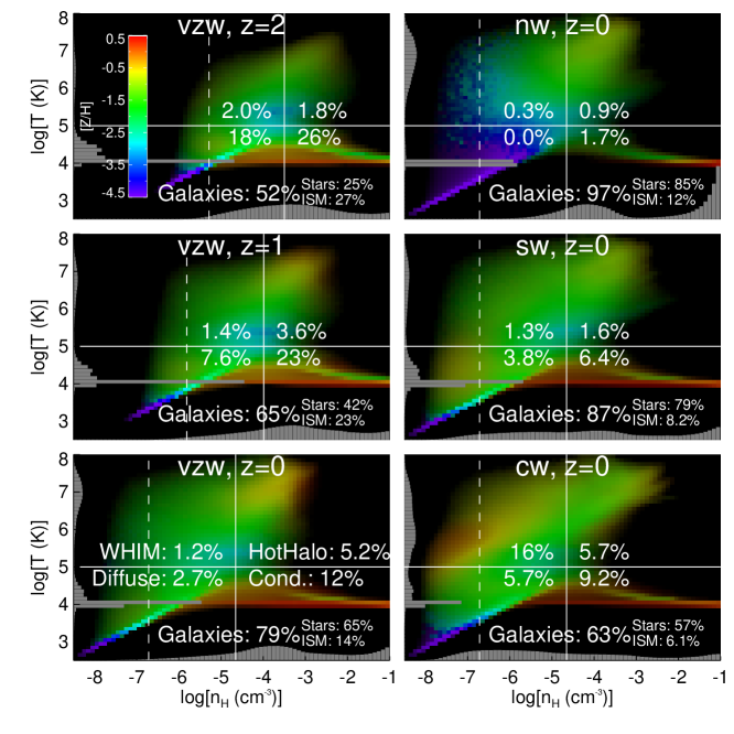
Figure 2: Density-temperature phase space diagrams showing the distribution of metals divided into four phases by the solid lines: horizontal divides “hot” and “cold” phases, and vertical divides halo and IGM phases. Colour indicates metallicity, and brightness corresponds to the baryon fraction. Percentages indicate the fraction of global metals in each phase (bottom right- condensed, bottom left- diffuse, top left- WHIM, top right- hot haloes, plus the percentage in galaxies subdivided into stars and ISM is also listed). Grey histograms show the gaseous metal fraction as a function of density ($x$-axis) and temperature ($y$-axis) including only metals outside galaxies. The vertical dashed line corresponds to the mean overdensity of the Universe. The left panels show the evolution of the momentum-conserved wind (vzw) model at $z=2,1,0$ and the right panels show the three other wind models at $z=0$ (nw- no winds, sw- slow winds, & cw- constant winds).

Examining the evolutionary trends in the vzw model, we see that the fraction of metals in the diffuse IGM drops rapidly with time, from 18% to 3% from $z=2\rightarrow 0$. In contrast, the fraction in the WHIM phase is quite small ($\sim 1-2\%$) and evolves downwards more slowly. Recall from D10 that the mass fraction of the WHIM in this model increases from $10\rightarrow 24\%$ during this time, while the fraction in the diffuse gas drops from $73\rightarrow 41\%$. Hence overall, the fraction of metals in the IGM (i.e. diffuse+WHIM) drops, a trend that is accentuated in the diffuse phase by a drop in the baryonic mass fraction in this phase, while for the WHIM the trend is countered by an increasing mass fraction. The decrease in the IGM metal fraction is balanced by an increase in the metal fraction in galaxies, from half at $z\sim 2$ to almost $80\%$ at $z=0$. Hence, from $z=2\rightarrow 0$, fractionally the metals move from low-density regions to higher density regions. We emphasise, however, that galaxies continue to enrich the IGM up to the present day and that the metallicity of the IGM does not actually decline; only the fraction of metals in the IGM declines. We return to this point in §3.3.

By $z=0$, we see that all the wind models have most of their metals within galaxies. In the no-wind case, only 3% of all metals are outside of galaxies, while in the cw case it is 37%. The momentum-conserved and slow wind models are intermediate, with 10–20% of their metals outside of galaxies. Still, these $z=0$ numbers are not large; in all the wind models more metals are outside of galaxies at high-$z$. This means that the solution to the “missing metals” problem (, 2007, 2007) at early epochs depends more on the accounting of metals outside of galaxies than today.

Examining the temperature histograms along the $y$-axis (including only metals outside galaxies), we see that the gas-phase cosmic metals in all the models at all epochs have a maximum at $T\sim 10^{4}$ K. This is an artificial temperature floor, since we do not include radiative cooling below $10^{4}$ K; however, this also is nearly the equilibrium temperature where cooling equals photo-heating. We will show in §6.2 that when we examine models including metal-line cooling below $10^{4}$ K from (2009b), metals cluster around $\sim 10^{4}$ K, although with more variable temperatures extending above and below owing to different equilibrium temperatures dependent on density and metallicity.

The central result is that most cosmic metals are not in hot gas, either in the WHIM or hot halo gas. At $z=0$, the IGM metallicity distribution for all wind models has a bimodal temperature distribution, with cool metals mostly at $T\sim 10^{4}$ K and hot metals mainly residing at intracluster medium (ICM) temperatures ($T\ga 10^{6}$ K). Few metals reside in between $10^{5}$ K and $10^{6}$ K (except in the cw case) because metal-line cooling is very efficient there, causing metal enriched gas to rapidly transition through these temperatures (OD09). In §7.2, we state that the bimodality is stronger in our simulations compared to simulations that explicitly smooth metals, because metals confined to individual SPH particles cool more rapidly over this intermediate temperature range.

The density histograms along the bottom of Figure 2 for the vzw model (left panels) show a peak in metal fraction at $n_{\rm H}\sim 10^{-3}-10^{-4}\;{\rm cm}^{-3}$ at all redshifts. This corresponds to an increasingly higher overdensity towards lower redshifts, reflecting the result from (2007) that the peak overdensity of metals increases with time. This is qualitatively true in the other wind models as well (not shown), although the actual distribution of metals in overdensity depends strongly on the particular wind model as we discuss in §3.2.

Figure 3 shows the mass fraction (left panels) and mass-weighted mean metallicity (right panels) of six baryonic phases (stars-top, ISM-2nd, diffuse-3rd, WHIM-4th, hot halo-5th, & condensed-bottom panels) for our four wind models, from $z=4\rightarrow 0$. At early epochs, star-forming gas holds the majority of metals. As time passes, metals become progressively locked up into stars, so that by $z=0$ stars contain the majority of cosmic metals. Outflows suppress the metal content in stars and the ISM somewhat but do not alter the overall trends. The mean stellar and ISM metallicities increase slowly from $z=4\rightarrow 0$, but even at early epochs it is already close to solar, and by today it exceeds solar. This is consistent with the early, rapid enrichment in galaxies typical in these models (e.g. , 2006, 2010) and is relevant for the IGM because it shows that the material expelled from galaxies has near-solar metallicities at all epochs. The metallicity of the IGM depends then on how far the metals are driven, and how they mix with the unenriched ambient gas.

The metal fraction of the IGM phases (diffuse+WHIM) generally drops from $z\sim 3\rightarrow 0$ in the wind models. This reflects the increasing difficulty that metals have in escaping from the denser regions where they are formed to less dense regions, as depicted in Figure 2. While the fraction of metals in the IGM phases is generally not large, it is still sufficient to reproduce the observations of metal-line absorbers across cosmic time (e.g. , 2006, 2009).

For the WHIM and hot halo phases, the $\delta_{\rm th}$ threshold that divides these two phases, first introduced in D10, makes a stark difference in the WHIM metal content compared to previous WHIM definitions without such a density threshold. The WHIM, which contains 24% of $z=0$ vzw baryons, holds only 1.2% of the $z=0$ metals and remains steady at [Z/H]$\sim-1.8$ since $z=4$. The WHIM forms through shock-heating owing to the gravitational collapse of large-scale structures (, 1999, 1999, 2001, 2006) while metal-enriching galactic outflows contribute fractionally less to the WHIM at late times (, 2008; Cen & Chisari, 2011). The metal content of the hot halo phase steadily increases, and by $z=0$ it holds more metals than the combined IGM phases (cf. 5.2% vs. 3.9% for vzw). The $y$-axis histograms for the vzw model clearly show the growing importance of hot halo metals from $z=2\rightarrow 0$. The $z=0$ panel indicates that most of these metals are at $T\ga 10^{6}$ K and hence are in the intragroup or intracluster medium (ICM). In all the wind models, the hot halo metallicity reaches 0.1 $\;{\rm Z}_{\odot}$ at $z=0$, but it also shows a density gradient such that the portion that would emit most strongly in X-rays has [Z/H]$\sim-0.5$ (see Figure 2). This is comparable to the measured metallicity of the ICM (e.g. Fukazawa et al., 1998; Peterson et al., 2003) and reconfirms that these simulations can generally reproduce the observed ICM metallicities (, 2008).

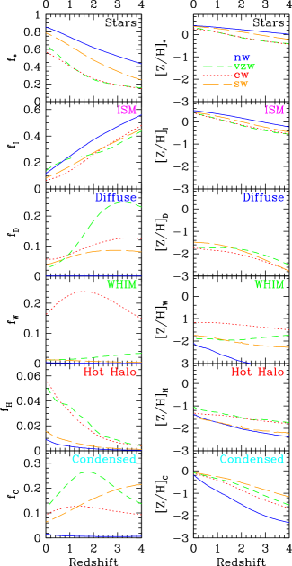
Figure 3: The evolution of metal mass fractions (left) and mass-weighted mean metallicity (right) of the four wind models from $z=4\rightarrow 0$ subdivided by phase (1st-stars, 2nd-ISM, 3rd-diffuse, 4th-WHIM, 5th-hot halo, & 6th-condensed). Four wind models are shown: solid blue- no-wind, dashed green- momentum-conserved winds, dotted red- constant winds, and long-dashed orange- slow winds.

More broadly, the fraction of metals in the IGM increases at very early epochs as winds enrich diffuse cosmic gas (, 2009), but then at later epochs the metals do not escape their haloes so easily or else re-accrete back into haloes. Hence, the metal fraction in the diffuse phase peaks at $z\sim 3-4$ in these wind models (Figure 3). Meanwhile, the metallicity in all the phases increases, but slowly; the most rapid increase is in the condensed phase gas, since this halo gas continues to be enriched even to late times by outflows. These trends, while generally true, are in certain aspects quite sensitive to the wind model, as we will discuss next.

3.2 Dependence on the Galactic Wind Model

The value of studying enrichment patterns lies in their high sensitivity to galactic winds, upon which the process of galaxy formation heavily depends (e.g. , 2010, 2010). We now contrast our vzw simulation to the three other wind models. The no-wind model produces nearly twice as many stars and metals as any wind model, and is incapable of enriching the diffuse IGM appreciably at any redshift, leaving it mostly pristine even by $z=0$ (Figure 2, upper right). The necessity to enrich the diffuse IGM to levels of at least [Z/H] $=-3$ at $z\geq 2$ (e.g. , 2003, 2004) is the main empirical requirement for large-scale galactic outflows. The diffuse phase metallicity of the nw model remains below the y-axis in Figure 3, only reaching [Z/H] $=-6.1$ at $z=4$ and $-3.9$ by $z=0$. This model does, however, achieve a hot halo metallicity comparable to our other feedback models, indicating that the enrichment of group and cluster haloes at least in part owes to a mechanism other than galactic outflows, such as dynamical stripping. (2008) showed that their no-wind model reached observationally reasonable [Fe/H] abundances via delayed Type Ia SNe from intragroup/intracluster stars, but [O/H] abundances were too low compared to observations and the baryonic fraction in stars was too high. Overall, the no-wind model strongly fails to match basic observations of both galaxies (e.g. Davé et al., 2011a) and the IGM.

The constant wind (cw) model has a high wind speed of ${v_{\rm wind}}=680\;{\rm km}\,{\rm s}^{-1}$ emanating from every galaxy, which pushes shock-heated metals into voids. This leads to a WHIM metal mass fraction more than 10 times higher than any other model (Figure 3, middle panel). These metals remain hot, because adiabatic cooling from Hubble expansion is not sufficient to return this gas to the photo-ionised IGM equation of state (EoS; , 1997, 2000) within a Hubble time. The excess heating is also reflected in the phase space diagram for this wind model (Figure 2, lower right), which has a high-metallicity peak in underdense regions at $T\sim 10^{6}$ K. The fast winds also increase the WHIM baryon percentage from 23 to 33% (compared to the nw model), whereas the vzw and sw models increase the WHIM baryonic fraction by one tenth as much, a 1% increase (D10). As (2006) show, a similar model with somewhat lower wind speeds (${v_{\rm wind}}=484\;{\rm km}\,{\rm s}^{-1}$) produces C iv absorbers at $z\sim 3$ that are are too wide compared to the observations, indicating that there is too much IGM heating at this early epoch.

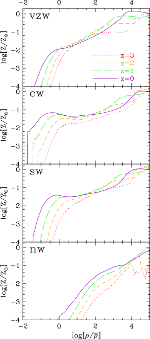
Figure 4: Mass-weighted mean metallicity as a function of overdensity from $z=3\rightarrow 0$ for the four models: momentum-conserved winds (vzw), no winds (nw), constant winds (cw), and slow winds (sw).

The slow wind (sw) model with ${v_{\rm wind}}=340\;{\rm km}\,{\rm s}^{-1}$ does not overly heat the early IGM, and in some sense represents a hybrid of the vzw model (similar average wind velocities) and the cw model (same mass loading). Like cw, this model creates a concentration of shock-heated metals ($T\sim 10^{4.5}$ K) in voids, but it is at lower temperatures and is much less prominent owing to the sw model’s lower wind speeds. In this model low-mass galaxies eject winds at high velocities relative to their escape velocity and high-mass galaxies, typically in dense environments, eject winds at less than the escape velocity. Hence, the sw model cannot populate the ICM with metals and, therefore, the metal phase space diagram in this regime mimics that of the no-wind model.

In the vzw model, winds from small galaxies have lower velocities. Hence they deposit metals at higher densities where metal-line cooling is efficient and can return these metals to $T\sim 10^{4}$ K. In hot gas, the vzw model produces a strong metallicity-density gradient by $z=0$ owing to its high outflow velocities from massive galaxies. Winds with $>1000\;{\rm km}\,{\rm s}^{-1}$ speeds emanating from these galaxies rarely escape the halo owing to the intervening halo gas, but they do shock heat to temperatures high enough that the cooling times are long, and hence the metals do not re-accrete onto the galaxies.

Figure 4 shows the mean metallicity-density relation in our four wind models from $z=3\rightarrow 0$. The no-wind model fails to provide widespread IGM enrichment, but even dynamical processes can deposit a smattering of metals at the cosmic mean density by $z\sim 0$. All the wind models show increased metallicities at all the plotted overdensities relative to the no-wind case. The constant wind model results in a curious upturn in the mean metallicity at void densities ($\rho<\bar{\rho}$), which is a generic feature of strong feedback models (e.g. Cen & Chisari, 2011, their Figure 24). Unfortunately this is very difficult to probe observationally using UV resonance lines owing to the low densities, as we will discuss in §5. The slow wind model has a less pronounced upturn, and it shows a less widespread metal distribution particularly at early epochs owing to its lower wind speed. The vzw model shows an interesting trend with overdensity, and the metallicity in filaments ($1\la\rho/\bar{\rho}\la 100$) is nearly time-invariant. Continual enrichment from galaxies pumps metals into these regions, but this is approximately balanced by gravitational effects that draw the metals back closer to galaxies and by the accretion of more pristine gas. At higher overdensities, the mean metallicity increases with time, while at sub-mean densities, metals slowly diffuse deeper into voids (, 2006). The differences between the models offer an opportunity to probe outflows if the metallicity-density relation and its evolution can be reliably measured, which is a central goal of IGM enrichment observations.

Overall, the evolution of metal content by phase shows much more dependence on feedback than our corresponding study of the abundance of baryons by phase (D10). While all the wind models significantly suppress the global star formation rate and hence metal production, the distribution of metals in the IGM shows clear differences. The velocity of the outflow and its motion through the ambient gas determines to what temperature the gas is shock heated and to what overdensity it reaches. Gas in sufficiently dense regions cools quickly, particularly since it is enriched. Hence, the outflow parameters critically determine the enrichment history of baryons outside of galaxies, providing an opportunity to constrain such parameters based on observations of IGM metal lines.

3.3 Outside-In IGM Enrichment

A generic feature of our IGM enrichment models is that they have a very early epoch where metals are distributed outwards into the IGM, but over most of cosmic time the newly produced metals became confined to ever decreasing regions around the galaxies that produced them. We call this “outside-in” IGM enrichment, and it has consequences not just for how metals enrich the IGM, but for how wind material re-accretes onto galaxies (, 2010).

We have already seen trends exemplifying outside-in enrichment above. The metal mass fraction in the IGM decreases steadily since $z\sim 3$, and the peak overdensity of metals increases with time. (2008) showed that the median distance reached by vzw outflows (with a wide dispersion) is $\sim 100$ physical kpc, implying widespread enrichment (in a comoving sense) early on and more confined enrichment at later epochs. The evolution of the vzw metallicity-density relationship in Figure 4 (top panel) shows that metals are in place at IGM overdensities at $z=3$ and that the metallicity is mostly invariant and actually declines slightly at $\rho/\bar{\rho}\sim 2-10^{3}$ from $z=2\rightarrow 0$. Newly produced metals are mostly confined to their own haloes and fall back onto their parent galaxies primarily from these overdensities; however winds continue to enrich IGM densities until $z=0$, especially the winds from lower mass galaxies, often even reaching void densities. Additionally, some enriched WHIM material also falls into galaxy haloes and eventually onto the central galaxy.

Another view of outside-in enrichment is provided by the age of $z=0$ metals as a function of overdensity, shown in Figure 5, top panel. We define the metal age as the time since a wind particle has most recently been launched, which is a good indicator of the age for metals in the IGM as these baryons are almost entirely enriched by winds. The median age of wind-blown metals is shown by the solid lines, and the 16 and 84% cuts are indicated by the dashed lines for the vzw model.

Figure 5 shows directly that lower overdensities are enriched earlier, particularly in the vzw model. For this model, the typical age of metals in voids is $\sim 10$ Gyr, reaching a minimum of $\sim 1$ Gyr at overdensities of a few thousand. The constant-$\eta$ models show less dependence on age with overdensity in the IGM, though at higher overdensities the metal ages are again significantly younger. The evolution of the metallicity-density relation of the cw model (Figure 4) shows a significantly increasing metallicity within voids with time. Most metals were already in place at higher redshift in gas that continues to expand into voids by $z=0$, but galaxies continue to enrich void overdensities below $z=1$. The same trends are true for the sw model, but they are shifted to higher overdensities and younger ages owing to its weaker winds. While the median age trends with overdensity are statistically significant and indicative of the history of metal enrichment, the larger scatter in all models at most densities prohibits a direct mapping of an overdensity to an age for a given wind model.

Wiersma et al. (2010) find a similar age-density anti-correlation using their definition of mean enrichment redshift. Our definition of age is a lower limit compared to theirs, because we measure the most recent wind launch as opposed to the redshift-weighted enrichment age. Both methods will find similar ages for wind particles that rapidly enrich and launch once, as is typical for metals that escape galaxies at high-$z$, but we will find significantly younger ages for winds that recycle back onto galaxies and have multiple wind launches and enrichment epochs.

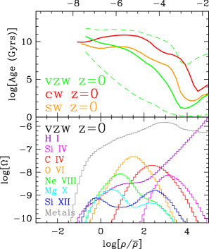
Figure 5: The top panel shows median ages of wind-blown metals at $z=0$ as a function of density (solid lines) with the 16th and 84th percentage cuts (dashed lines, vzw only) for the momentum-conserved winds (vzw, green), constant winds (cw, red), and slow winds (sw, orange). Lower overdensities are enriched earlier in all wind models in what we term “outside-in” enrichment. The bottom panel shows cosmic ion densities of vzw metal species as a function of density, as well as, H i (purple lines) and total metal density (grey lines). The two panels can be compared to show that in general higher ionisation species generally trace lower overdensities, which have older metals.

To relate the IGM metal age to observables, we plot in the lower panel of Figure 5 histograms of the $z=0$ vzw cosmic ion densities (in 0.1 dex bins of overdensity) for the ions that we follow and for H i. In general, higher ionisation metal species trace older IGM metals occupying lower overdensities in the vzw model. For example, observed Ne viii and O vi absorbers are likely to be tracing fairly old ($\ga 5$ Gyr) metals, while C iv and Si iv more often trace younger metals, although with a large age scatter. Every metal species shows a peak corresponding to the overdensity where the species is primarily photo-ionised. A second peak at higher overdensities for Si xii and Mg x corresponds to collisionally ionised metals inside haloes. Ne viii also shows an extended shoulder toward halo densities corresponding to collisionally ionised metals. This figure foreshadows our analysis in §5 showing that species including C iv, O vi, and Ne viii are primarily photo-ionised in our simulations. Interestingly, these three species exceed the cosmic density of H i at a range of IGM densities.

The idea that the IGM is enriched in an outside-in manner has a long history (Tegmark, Silk, & Evrard, 1993; Nath & Trentham, 1997; , 2001, 2002). In general, these models postulated that the IGM underwent widespread early enrichment typically during the reionisation epoch from some putative powerful source such as Population III stars, when halo potential wells were still small. Our model, while similar in character, is fundamentally different in that it does not invoke very early enrichment from mysterious sources. Instead, the outside-in pattern arises from the dynamics of galactic outflows from the epoch of early galaxies ($z\ga 6$) until today. The source of IGM enrichment is the observed population of high-$z$ star-forming galaxies that our simulations naturally reproduce (, 2006, 2007). Energetically moderate outflows from these galaxies enrich a small, but rapidly growing fraction of the IGM, in agreement with observed constraints from high-$z$ metal-lines (e.g. , 2009). These early outflows end up enriching a greater comoving volume than lower redshift outflows, which travel similar physical distances in our model (, 2008). In contrast, (2007) showed that enriching the IGM entirely prior to $z\sim 6$ would violate observations of the C iv enrichment at those epochs.

4 Metal-Line Observables

We present metal-line predictions for COS observations in this section along with comparisons to other pre-COS data. We consider statistics assuming a S/N=30 per $6\;{\rm km}\,{\rm s}^{-1}$ pixel in our simulated spectra, convolved with the COS line spread function (LSF) assuming the FUV G130M LSF at 1450Å, just as we did in D10. We model the LSF as a central peak with a $1\sigma$ Gaussian width of $\approx 17\;{\rm km}\,{\rm s}^{-1}$ and substantial non-Gaussian wings, keeping this fixed for all wavelengths to avoid introducing artificial evolution from a varying LSF.

We obtain line statistics by fitting Voigt profiles to individual components using AutoVP (, 1997). Each component has a fitted rest equivalent width ($W$), a column density ($N$), and linewidths ($b$-parameters). An absorption system is defined as all components that can be grouped together if they lie within 100 $\;{\rm km}\,{\rm s}^{-1}$ of another component. Systems are more easily comparable with observations, because data quality does not always allow the easy and consistent identification of components. For example, it can be easier to divide a system into more components if the S/N and resolution are higher. We sum up system column densities to calculate cosmic ion densities ($\Omega$). We discuss the equivalent width distribution of systems versus components for O vi, where observations for both have been quantified. We present results in this section for our four main simulations, plus a vzw model with turbulent broadening added after the completion of the simulation (OD09), motivated by the observed O vi linewidths.

4.1 Equivalent Width Distributions

Cumulative equivalent width distributions (EWDs), presented in Figure 6, show the frequency of systems greater than or equal to the $W$ indicated on the $x$-axis. They offer a simple and direct statistic to test theoretical models. We show EWDs of four metal lines: O vi 1032Å, C iv 1548Å, Si iv 1394Å  (all between $z=0-0.5$), and Ne viii 770Å  (at $z=0.5-1.0$). We show predictions for our four wind models and a fifth model (vzw-turb in cyan) of turbulent $b$-parameters ($b_{\rm turb}$) added after the completion of the simulation using specexbin (, 2009).

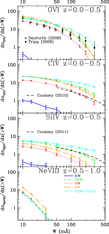
Figure 6: Cumulative equivalent width distributions of O vi (top), C iv (second), Si iv (third), and Ne viii (bottom) for our four wind models (solid blue- no-wind, dashed green- momentum-conserved winds, dotted red- constant winds, and long-dashed orange- slow winds, plus the vzw model with turbulent broadening (dot-dashed cyan). The line types correspond to the same models throughout the paper. Observations for O vi (, 2008, 2008) and C iv & Si iv (, 2010, 2011) are also plotted. For the first three panels, we count all lines in our continuous synthetic spectra out to $z=0.5$ and divide by $\Delta z=0.5$, while the fourth panel uses the same procedure for $z=0.5-1$. Error bars correspond to 1-$\sigma$ Poisson errors in the models and observations.

The EWDs with no winds (blue solid lines) exhibit far fewer absorbers than models with winds, and significantly underestimate the observations of O vi, C iv, and Si iv. In general, the cw model (red dotted lines) produce fewer absorbers than the other wind models because this wind model (i) produces less metals overall owing to its greater suppression of star formation and (ii) injects more of its metals into the low-density WHIM where they are unobservable using these transitions. Compared to vzw, the sw model creates fewer C iv and Si iv absorbers, which we will show in §5 trace the condensed phase within haloes that are enriched to higher levels by vzw winds. At the same time there exist more weak O vi and Ne viii lines in the sw model, because these arise from the diffuse phase that is enriched to higher levels via sw winds (cf. vzw and sw $z=0$ metallicity-density relations in Figure 4).

We discuss turbulence as a model variation in §6.3, but we present it here because this is part of our favoured model for O vi observations. We also show the effect on C iv, Si iv, and Ne viii, although we argue later that this model may not be applicable to absorbers tracing higher densities. As in OD09, adding $b_{\rm turb}<60\;{\rm km}\,{\rm s}^{-1}$ (see Equations 4 & 5 in §6.3) increases the number of absorbers above 100 mÅ , allowing us to fit the observed O vi EWDs, and it also blends some weaker components into stronger ones, thus reducing their numbers (cf. vzw and vzw-turb model in the top panel of Figure 6). C iv and Si iv also show a dramatic increase in the number of $\geq 100$ mÅ components if we apply this same density-dependent model.

The simulations presented here produce statistically identical O vi results to OD09 for the vzw model. However, the vzw model appears to over-produce the observed C iv, while the cw model provides a better fit to this data (, 2010). We predict that COS will make many Ne viii detections, especially between 10-20 mÅ. In general, the lithium-like ions are harder to detect for higher atomic numbers corresponding to higher ionisation species, because both their oscillator strengths and wavelengths decline, leading to smaller equivalent widths for a given column density.

4.2 Column Density Distributions

Column densities provide a more direct accounting of the amount of metals present than equivalent widths, but they are more difficult to obtain from observations as COS often does not resolve individual metal-line absorbers. Nevertheless, AutoVP fits column densities $N$ and linewidths $b$ for every component. Given that we have applied COS instrumental characteristics (albeit with a perhaps optimistic S/N ratio), these predictions should be representative of the level of information obtainable from (the very best) COS spectra. We emphasise that these are distributions of inferred column densities obtained by Voigt-profile fitting components and summing them together into systems, and not necessarily distributions of true column densities of physically identified, unblended components.

We display the differential column density distributions (CDDs) of systems in Figure 7. As in D10, we plot $f(N_{\rm ion})\equiv d^{2}n/dN_{\rm ion}dz$ multiplied by $N_{\rm ion}$ to improve the readability and to provide a dimensionless number that indicates the relative number of lines per unit redshift for a given $N_{\rm ion}$. Again our four basic wind models are plotted, along with turbulent broadening added to the vzw model. We show eight species over $\Delta z=0.5$ for a redshift range that falls within the COS far-UV (FUV) channel: O vi, C iv, Si iv, & N v all at $z=0-0.5$, Ne viii at $z=0.5-1.0$, and O v, Mg x, & Si xii at $z=1.0-1.5$.

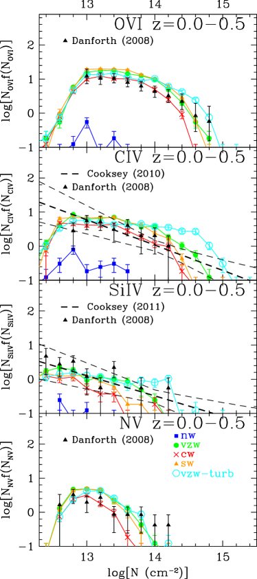
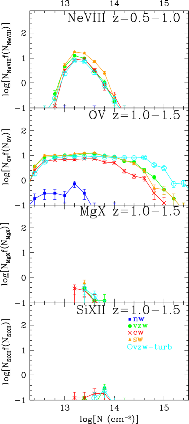
Figure 7: Column density distributions for our mock S/N=30 COS observations for six species: O vi 1032Å, C iv 1548Å, Si iv 1394Å, N v 1239Å, Ne viii 770Å, O v 630Å, Mg x 609Å, and Si xii 499Å. The four wind models and the turbulently broadened vzw model are generated from a path length of $\Delta z=35$ over a redshift range observable by the COS NUV channel. Data from (2008) (triangles) and (2010, 2011) (dashed lines, thin lines encompass the 1-$\sigma$ error range) are also shown. Our simulations do not include AGB production of N v, so these predictions should be taken as lower bounds. Error bars are 1-$\sigma$ Poisson errors.

The qualitative differences between the wind models and the data for the column density distributions are similar to those obtained for the equivalent widths as we discussed in the previous section. Without winds, very few IGM metal lines are present, and the predictions fall well short of available observations. The O vi CDD is consistent with the data (, 2008) for the vzw and vzw-turb models, but the same models produce too many C iv absorbers, especially above $10^{14}\;{\rm cm}^{-2}$, compared to the observations (, 2010). This disagreement is statistically significant, and further data from COS should provide much better constraints on weak C iv absorbers. Si iv predicts more strong lines and less weak lines than those observed (, 2011), though the discrepancy is not as large as with C iv, and the $z=0-1.2$ redshift range of this data set is larger and centred at much higher redshift than in our simulations ($\langle z\rangle\sim 0.9$ vs. 0.25). Despite the different redshifts for Si iv, our simulated Si iv CDDs remain statistically identical with $\langle z\rangle=0.75$ and $1.25$ over the column density range of detected absorbers (not shown).

We show N v CDDs but caution that we do not follow the unique chemodynamic origin of nitrogen from secondary enrichment sources (AGB stars). Hence, the Type II SNe origin assumed here for nitrogen likely represents a lower limit, as nitrogen is copiously produced in AGB ejecta (e.g. , 2001). Our models underestimate the (2008) statistics for higher N v columns, which appears to support this interpretation.

For Ne viii (upper right panel of Figure 7), pushing below $10^{13.8}\;{\rm cm}^{-2}$ is rewarding because the CDD rises sharply. At column densities $\ga 10^{14}\;{\rm cm}^{-2}$, the line counts are predicted to be well under one per unit redshift, but at $\sim 10^{13}\;{\rm cm}^{-2}$ there should be $5-10$ per unit redshift. Hence high S/N is essential to detect significant numbers of these absorbers. Note that our estimates are probably optimistic because we assume detection based on only the stronger component, but in actuality detection of the weaker 780Å component is usually required for a robust line identification.

We predict O v should be generously abundant in the spectra of $z\ga 1$ quasars probed by COS over a wide range of column densities. We show the 630 Å O v statistics, because it is likely representative of a large number of lower ionisation species with far-UV transitions that should contribute significantly to intervening absorption in higher redshift quasars probed by COS. O v should be among the strongest owing to a large oscillator strength and oxygen being the most abundant metal.

Mg x and Si xii absorbers are very rare in our sight lines and definitely require winds to be present at all. We find only 2 Mg x and 6 Si xii absorbers over $\Delta z=35$ with $W\geq 10$ mÅ in the vzw model. We argue in §5.1 that we may not be resolving the conductive interfaces from which very high-ionisation lines such as Ne viii and Si xii may arise, and hence that these absorbers may be more common than our current models predict.

Looking at the vzw-turb model, in theory the total column density should be conserved (unlike $W$) when adding turbulence in the way that we do using specexbin. But as one can see, in practice the column densities are increased when turbulence is added. This occurs because for strong saturated lines, which preferentially receive the largest turbulent contributions, AutoVP tends to fit a higher column density given only a single line with no doublet information. Also, weaker lines may become blended or harder to detect. Hence, there is a noticeable increase in the predicted line frequencies especially for C iv at $10^{14.0}\;{\rm cm}^{-2}$ and Si iv at $10^{13.8}\;{\rm cm}^{-2}$, which correspond to the column densities where these transitions fall off the linear curve of growth and begin to become saturated without turbulent broadening. COS spectra will be able to use the two doublet transitions to perform a curve of growth analysis and obtain more accurate $N$s for saturated components. Including such information in AutoVP may mitigate the increase seen at high-$N$; we leave such an analysis for a more careful comparison to real data.

4.3 Cosmic Ion Densities

Integrating over a CDD or summing the column densities of lines provides a global view of the amount of cosmic metal absorption. To obtain the cosmic density of an ion, we sum up all the absorber column densities between $10^{12-15}\;{\rm cm}^{-2}$ using

$$\Omega({\rm ion},z)={H_{0}m_{\rm metal}\over c\rho_{crit}}{\Sigma N({\rm ion},z)\over\Delta X(z)},$$ (3)

where $H_{0}$ is the Hubble constant, $c$ is the speed of light, $\rho_{crit}$ is the critical density of the Universe, and $m_{\rm species}$ is the atomic weight of the given species. $\Delta X(z)$ is the pathlength in a $\Lambda$CDM Universe where $X(z)=\frac{2}{3\Omega_{\rm M}}\sqrt{\Omega_{\rm M}(1+z)^{3}+\Omega_{\Lambda}}$. We evaluate Equation 3 from the Voigt-profile fitted column densities, just as is done for observations. We choose the column density range both for historical reasons (, 2001), and because it quantifies lower-column metal lines that are expected to arise in the IGM as opposed to those within the galactic ISM.

We bin the $\Omega_{\rm ion}$s in bins of $\Delta z=0.5$ and plot the points with error bars in Figure 8 for O vi, C iv, Si iv, and Ne viii. For simplicity, we use the same COS FUV instrument parameters for the entire $z=0-2$ range even though most redshifts fall outside of the COS wavelength range. We show the same four wind models as before, and also the vzw model with turbulent broadening. We also plot $\Omega_{\rm metal}$ computed by summing up the total mass density of all the SPH particles outside of galaxies ($n_{\rm H}<0.1\;{\rm cm}^{-3}$) for the appropriate metal species (continuous lines).

$\Omega_{\rm ion}$s usually do not change by much if we adjust the column density bounds from $10^{12}$ to $10^{13}\;{\rm cm}^{-2}$ or from $10^{15}\;{\rm cm}^{-2}$ to any higher value, because the vast majority of an ion’s cosmic density resides in $10^{13-15}\;{\rm cm}^{-3}$ components in S/N=30 spectra. The most dramatic exception is C iv at $z\ga 1$, which can increase by a factor of more than two when including lines above $N_{\hbox{C\,{\sc iv}}}>10^{15}\;{\rm cm}^{-2}$.

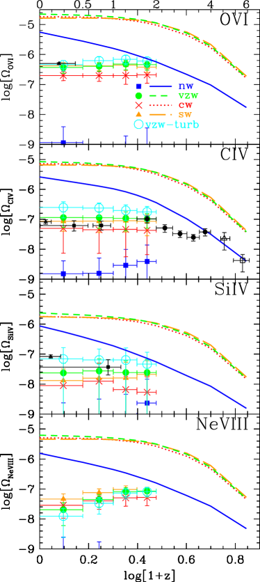
Figure 8: Cosmic ion density evolution of O vi (top), C iv (second), Si iv (third), and Ne viii (bottom) for the same models described in Figures 6 and 7. Large symbols show simulated $\Omega_{\rm ion}$s calculated from S/N=30 COS spectra, with horizontal error bars indicating $\Delta z=0.5$ bins and vertical error bars indicating the variance among $\Delta z=0.5$ sight lines. Continuous lines show the evolution of $\Omega_{\rm metal}$ calculated by summing up all the mass outside galaxies of oxygen (top panel), carbon (second), silicon (third), and neon (bottom). Data are from (2008) (solid triangles), (2010, 2011) (solid squares), (2010) (solid circles), (2003) (open triangle), and (2009) (open square) and are all scaled to a $\Omega_{\rm M}=0.28$, $\Omega_{\rm\Lambda}=0.72$, $H_{0}=70\;{\rm km}\,{\rm s}^{-1}$ cosmology. Redshifts are listed on the top axis.

Models with outflows produce roughly constant $\Omega_{\hbox{O\,{\sc vi}}}$ and $\Omega_{\hbox{C\,{\sc iv}}}$ from $z=2\rightarrow 0$, and agree with observations where available. While O vi agrees with the data in all three observables thus far explored, C iv only agrees for $\Omega_{\hbox{C\,{\sc iv}}}$ because too many weak and too few strong absorbers exist compared to the current data (, 2010). In general, the non-evolution in these species reflects the non-evolution in the total mass densities of metals outside of galaxies ($\Omega_{\rm metal}$s, lines in Figure 8), but the ion densities are shifted lower by a factor of $\sim 30-100$. The majority of the Universe’s metals are produced after $z=2$, but this is offset by more metals remaining nearer to galaxies and being reincorporated into stars, i.e. “outside-in” enrichment. Note that the ratio $\Omega_{\rm metal}/\Omega_{\rm ion}$ cannot be treated as a global ionisation correction for an ion (e.g. C/C iv or O/O vi), because we will show in §5.2 that $\Omega_{\rm ion}$ calculated using Equation 3 does not recover the total cosmic density of that ion.

In contrast to the other ions shown, $\Omega_{{\hbox{Ne\,{\sc viii}}}}$ shows a steady decline from $z=1.5\rightarrow 0$ for the vzw model. The photo-ionised Ne viii component is within the detection limits of COS at higher redshift, and becomes harder to detect at low redshifts at wavelengths only accessible using the Space Telescope Imaging Spectrograph (STIS) and the Far UV Spectroscopic Explorer (FUSE). Observing Ne viii at wavelengths between 1100-1700Å with COS could be ideal to trace the peak in $\Omega_{{\hbox{Ne\,{\sc viii}}}}$.

The turbulent vzw model predicts higher $\Omega$s than the vzw model even though the total column density theoretically should be preserved. As explained previously, the broader profiles with turbulent broadening are fitted more accurately by AutoVP than unbroadened thin saturated profiles. This is especially true if the cosmic density of an ion is dominated by a few strong absorbers.

In summary, outflows are generically required to enrich the IGM as observed, and there is a mild sensitivity in observations of $W$, $N$, and $\Omega_{\rm ion}$ to the particular form of galactic outflows employed. While momentum-conserved winds plus turbulence best matches the O vi data (as it was in part designed to do), it overproduces C iv and Si iv absorption. Ne viii shows a particularly steep column density distribution owing to a preponderance of weak photo-ionised lines, motivating deep observations to detect this interesting IGM tracer. The cosmic metal density is generally constant from $z\sim 2\rightarrow 0$, in contrast to its marked rise from $z\sim 6\rightarrow 2$ (, 2006, 2008), and this is broadly reflected in the constancy of $\Omega_{\rm ion}$ for most ions over this redshift range.

4.4 Component Linewidths

Component linewidths ($b$-parameters) are also fit with AutoVP, but are almost always dominated by the COS LSF (the instrumental $b\sim 24\;{\rm km}\,{\rm s}^{-1}$); therefore, linewidths are often much wider than they are in STIS data. We show the linewidth histograms for the simulations with winds in Figure 9 along with the vzw-turb model, which uses the turbulent broadening model motivated by OD09 to match the observed $b$-parameters of STIS O vi absorbers, but now applied to all ions. The histograms apply to all O vi, C iv, and Si iv absorbers with $W\geq 30$ mÅ between $z=0-0.5$, and Ne viii absorbers with $W\geq 10$ mÅ at $z=0.5-1.0$.

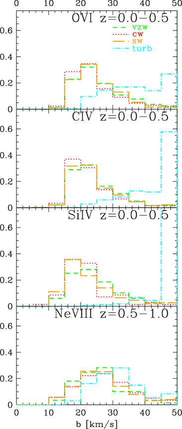
Figure 9: Simulated COS linewidth histograms for O vi (top), C iv (second), and Si iv (third) between $z=0-0.5$ for all components with $W\geq 30$ mÅ and Ne viii (bottom) for components between $z=0.5-1.0$ and $W\geq 10$ mÅ. The three models with winds and the turbulently broadened vzw model are generated from a path length of $\Delta z=35$ over a redshift range observable by the COS NUV channel. Note that these linewidths are not corrected for the instrumental broadening by the COS LSF, which has $b\approx 24\;{\rm km}\,{\rm s}^{-1}$.

Without turbulent broadening, the linewidths of the three wind models are nearly identical. The COS LSF makes it difficult to determine temperatures from thermal broadening in our case since we show in the next section that the majority of our absorbers are near $T\sim 10^{4}$ K, corresponding to linewidths much smaller than the LSF. We do not show the nw model owing to its low number statistics.

Adding turbulence using the heuristic prescription of OD09 dramatically alters the $b$-parameter histograms for not just O vi, to which this prescription was calibrated, but even more so for C iv and Si iv. AutoVP fits a maximum $b=50\;{\rm km}\,{\rm s}^{-1}$, which means that the majority of C iv and Si iv absorbers in the 45-50 $\;{\rm km}\,{\rm s}^{-1}$ bin may even be wider. Unlike thermal broadening, turbulent broadening is independent of the atomic species, and the broader linewidths for C iv and Si iv are a result of the OD09 turbulence model, which adds wider $b_{\rm turb}$ to higher density gas. We argue in §6.3 that such wide absorbers likely represent a break-down of the turbulence model, because while there are few published observed linewidths of these species, thinner line profiles are apparent in the data (e.g. , 2010). Ne viii absorbers are not as sensitive to the turbulence model, because they arise from lower densities where $b_{\rm turb}$ is small.

4.5 Components & Systems

The choice to group components into systems or treat them individually is an important consideration when comparing simulations to observations. K. Cooksey (private communication) advises us that it is more proper to compare grouped systems to the data of (2010, 2011), because they group components into systems if they lie within a few tens of $\;{\rm km}\,{\rm s}^{-1}$. (2008) groups metal-line components together into systems if their associated ${\rm Ly}\alpha$ lines lie within $50\;{\rm km}\,{\rm s}^{-1}$ of each other (C. Danforth, private communication). (2008) publish both component and system EWDs, which we show in Figure 10.

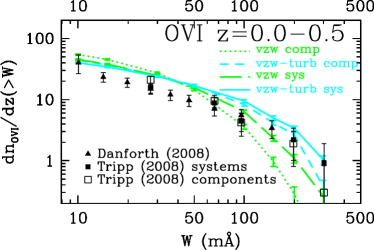
Figure 10: Cumulative equivalent width distributions of O vi components and systems quantified in our simulations for the vzw and vzw-turb models. Observations of (2008) have both system (filled square) and component (open square) distributions. Data from (2008) (triangles) groups components based on the associated H i identification.

The vzw model indicates how important it is to compare the appropriate component and system EWDs. The vzw system EWD would agree with the component EWD of (2008), but the appropriate comparison, the vzw component EWD, under-predicts the strongest observed O vi components. The shortfall of strong $W$ components was part of the motivation for OD09 to attempt the vzw-turb model (the other motivation being mismatched linewidths). The vzw-turb makes less of a difference between the two types of EWDs, because turbulent broadening increases the component $W$s so that the strongest component of a system becomes more dominant relative to weaker components; thus the strongest component more likely sets the system $W$ resulting in less differences between the two methods. The trend of this model’s component and system EWDs matches that of (2008), although we appear to consistently over-estimate component and system frequencies at $\leq 100$ mÅ.

The comparison to (2008) is more difficult because their search relies on the identification of the associated H i absorption, but their measurements appear consistent with (2008) systems. We also tested the choice of grouping components within 250 $\;{\rm km}\,{\rm s}^{-1}$ instead of 100 $\;{\rm km}\,{\rm s}^{-1}$, but this makes almost no difference and gives statistically identical results. If components lie close to each other, they are almost always within 100 $\;{\rm km}\,{\rm s}^{-1}$ of another component.

5 Metal-Line Absorber Physical Conditions

We now link the observed metal-line absorber characteristics with their physical conditions just as we did for ${\rm Ly}\alpha$ absorbers in §5 of D10. We concentrate on ion mass density-weighted physical parameters, mainly hydrogen density and temperature, using the same method described in OD09. This weighting procedure sums the ion mass density, and hence absorption, of every SPH particle contributing at the line centre of an identified absorber, accounting for peculiar velocities and temperature broadening. This procedure is similar to the optical depth-weighting of Tepper-Garcia et al. (2011) with the only difference being that they sum physical quantities from each pixel across a line profile whereas we use the value at the line centroid. Tepper-Garcia et al. (2011) find that the difference between these two methods is small, so the methods should be comparable. We consider all absorbers where the strongest line transition has $W\geq 10$ mÅ in our 70 S/N=30 COS sight lines.

5.1 Absorbers in Phase Space

Figure 11 displays total metals (top panels) and selected ions (middle and bottom panels) in density-temperature phase space at $z=0.2$ (left) and $z=1.0$ (right). The grey pixelated shading is the fractional $\Omega$ summed from SPH particles binned in $0.1\times 0.1$ dex pixels. The temperature bimodality of metals described in §3.1 is obvious at both redshifts, with the metals pushing to lower densities and higher temperatures with time.

We show the phase space occupied by C iv and O vi absorption at $z=0.2$ as the grey shading in the middle left and bottom left panels, respectively. These ions trace gas in a limited range in phase space, particularly weighted towards the cooler gas. Overlaid using coloured open circles are the ion mass density-weighted hydrogen densities and temperatures of simulated absorbers over a pathlength of $\Delta z=14$ (70 sight lines over $z=0.1-0.3$). Colour and circle size both scale with the absorber column density as indicated by the legend above each panel.

Our identified absorbers overlap with the darkest shading, which provides a consistency check that our ion weighting accurately captures the physical conditions of the absorbers. The two sets of histograms along the $x$-axis (for density) and $y$-axis (for temperature) directly compare the SPH-summed quantities (solid grey histograms) and the absorber-summed quantities (open red histograms); the amplitudes of these histograms can be directly compared. For example, the mismatch of C iv density histograms in denser halo gas indicates that summing the halo C iv absorbers (red) underestimates the true $\Omega_{\hbox{C\,{\sc iv}}}$ arising from this phase (grey). The temperature histograms show that most of this missing absorption is between $10^{4.0-4.1}$ K. The same is true for Si iv probing even higher densities (not shown). The main cause for this is that saturated absorbers tracing halo gas have their column densities underestimated without turbulent broadening, which is apparent in the differences between the vzw and vzw-turb CDDs in Figure 7. The mismatch is less severe but still noticeable for O vi.

At $z=0.2$, both C iv and O vi predominantly trace the cooler phases of gas at temperatures closer to $10^{4}$ K than $10^{5}$ K. N v (not shown) traces the same temperatures, but at intermediate overdensities between C iv and O vi. For O vi, this is in marked contrast to some previous work (Cen & Chisari, 2011; , 2011; Tepper-Garcia et al., 2011), all of whom find most of their O vi at $T>10^{5}$ K at the same redshifts. We believe it is the interplay of our momentum-conserved winds with the cooling rates in the $T\sim 10^{5}$ K regime that results in our differing conclusion. We will show in §6.2 that using the photo-ionised metal-line cooling rates of (2009b) does not fundamentally change the phase space traced by O vi absorbers in our vzw model. Hence, we reiterate the conclusion by (2009) that, for a physically well-constrained outflow model, O vi primarily traces diffuse, photo-ionised metals.

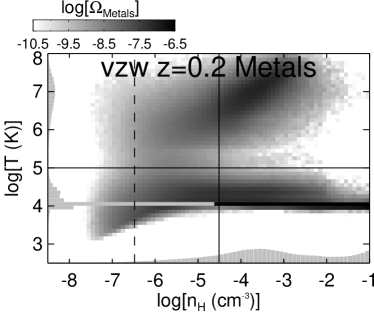
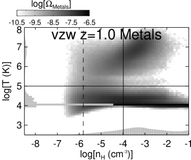
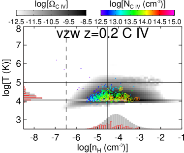
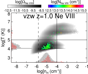
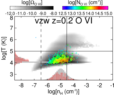
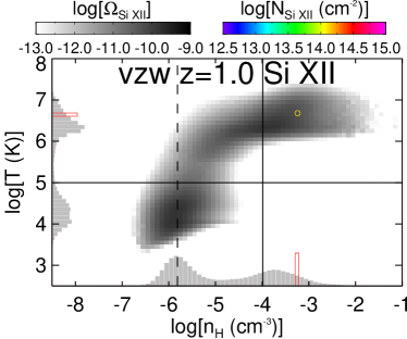
Figure 11: $\Omega$ phase space diagrams at two redshifts (left- $z=0.2$, right- $z=1.0$) for all metals (top) and two common ion species observable with COS at each redshift (centre and bottom) from the r48n384vzw model. Grey shading indicates the fractional $\Omega$ summed from all SPH particles binned in $0.1\times 0.1$ dex pixels, and grey histograms show the distributions in density and temperature for the metals and each ion species. Overlaid coloured circles are simulated COS absorbers over $\Delta z=0.2$ for 70 sight lines where S/N=30. Colour and symbol size scale with absorber column density. Red histograms count the summed $\Omega$s of absorbers as functions of density and temperature, calibrated to the same scale as the grey histograms using Equation 3 and are directly comparable to test how well simulated observations recover the total ion density contained in the simulations. Solid lines correspond to the division of the four phases as in Figure 2, and the dashed vertical lines indicates mean overdensity.

We show two higher ionisation species, Ne viii and Si xii, at $z=1.0$, because this is the redshift where COS is able to observe these lines. The Si xii doublet at 499.3,521.1Å falls into the COS sensitivity range at $z>1.1$, but we show simulated absorbers and phase space centred at $z=1.0$ because these characteristics are not strongly evolving. Si xii has a larger fraction of mass arising from collisional ionisation at densities corresponding mostly to halo gas.

Surprisingly, most simulated Ne viii absorbers are predicted to be photo-ionised, tracing overdensities of around $\delta\sim 10$. However, the strongest simulated absorber is at $N_{{\hbox{Ne\,{\sc viii}}}}=10^{14.2}\;{\rm cm}^{-2}$ tracing $T=10^{5.8}$ K gas, and is likely more representative of the three Ne viii absorbers (, 2005; Narayanan et al., 2009, 2011) already observed, since it has a similar column density and hence probably a similar environment. Mulchaey & Chen (2009) find a 0.25 $L^{*}$ galaxy at an impact parameter of 73 $h^{-1}{\rm kpc}$ at nearly the same redshift as the $z=0.207$ Ne viii absorber along the HE0226-4110 sight line, suggesting that this absorption originates in collisionally ionised halo gas. They further suggest that the origin is a conductive interface between cool clouds moving through a hot medium, based on the alignment of Ne viii with lower ionisation species, something that would not be captured in our simulations. Narayanan et al. (2011) note the existence of a 0.08 $L^{*}$ galaxy at 110 kpc at $\delta v=180\;{\rm km}\,{\rm s}^{-1}$ from the Ne viii absorber at $z=0.495$ in the PKS0405-123 sight line, and further argue this is likely tracing $T\sim 10^{5.7}$ K gas either in a hot halo or nearby WHIM.

We emphasise that our model predicts numerous weaker Ne viii absorbers tracing the diffuse photo-ionised component, as a separate and probably as yet undetected population. These absorbers are mainly below $N_{{\hbox{Ne\,{\sc viii}}}}=10^{13.7}\;{\rm cm}^{-2}$ (cf. $10^{13.85}$, $10^{13.98}$, $10^{13.96}\;{\rm cm}^{-2}$ for the discovered systems mentioned above) and should arise outside haloes. We cannot distinguish any other obvious observational characteristics between the two types of Ne viii absorbers, as the simulated $b$-parameters at COS resolution do not straightforwardly translate to temperature. Alignment with H i absorbers tracing overdensities of $\sim 10$, i.e. $N_{{\hbox{H\,{\sc i}}}}\sim 10^{13.5}\;{\rm cm}^{-2}$ at $z=0.75$, is common for the photo-ionised Ne viii absorbers. Upcoming deeper COS observations might be able to detect this population.

The true frequency of hot Ne viii absorbers may exceed our predictions given that our simulations do not adequately resolve conductive interfaces within haloes. Narayanan et al. (2009) estimates a higher frequency below $z<0.5$, although their estimate is based on one absorber and is highly uncertain. Additionally, we predict a mass density of $\Omega_{{\hbox{Ne\,{\sc viii}}}}$ at $z=1.0$ almost $3$ times higher than at $z=0.2$, which is suggestive of an even greater frequency of such absorbers at high redshift; the increase is primarily from the increased neon traced in the photo-ionised component. Given their distinct phase spaces (hot halo and dense WHIM vs. diffuse), the potential for absorber bimodality is greater than for O vi, but identifying it may require direct observation of an absorber’s environment. We will return to this discussion in a future paper discussing the galaxy-absorber connection.

5.1.1 Photo-ionised Absorption

It may initially be surprising that high ionisation species such as Ne viii, Mg x, and Si xii can be excited via photo-ionisation given their high ionisation potentials, but the existence of such absorbers is straightforwardly traceable to the shape of the (2001) background. We demonstrate this in Figure 12, where we show the Line Observability Index (LOX, Hellsten et al., 1998)– the predicted equivalent width of metals lines associated with H i if the IGM is uniformly painted with a metallicity of $Z=0.1\;{\rm Z}_{\odot}$ and with a uniform temperature of $T=10^{4.2}$ K. Although these assumptions are overly simplistic, they are representative and serve to illustrate the main point.

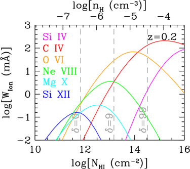
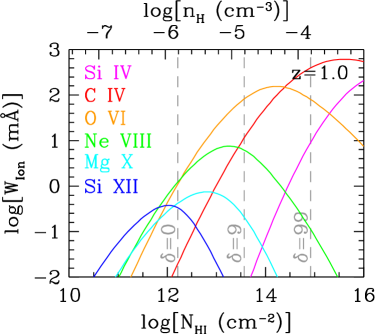
Figure 12: Line Observability Indexes (LOXs) at $z=0.2$ and 1.0 showing the photo-ionised equivalent widths for a variety of metal species as a function of H i column density assuming the density-$N_{{\hbox{H\,{\sc i}}}}$ relation from Equation 3 of D10, $Z=0.1\;{\rm Z}_{\odot}$, $T=10^{4.2}$ K for the metal species, and a (2001) background renormalised to match the vzw ${\rm Ly}\alpha$ forest flux decrement (D10).

At $z=1.0$, Ne viii peaks near $n_{\rm H}\sim 10^{-5.0}\;{\rm cm}^{-3}$ with equivalent widths as high as 8 mÅ. Our simulated photo-ionised Ne viii absorbers are stronger than this owing to the inhomogeneous enrichment, which results in higher metallicities for the detected absorbers, and furthermore arise at slightly higher densities owing to the positive metallicity-density gradient present in the vzw models (, 2006). Photo-ionised Si xii should exist around the mean density (assuming the metallicity is sufficiently high), but it should not exceed even 1 mÅ, well below the detectability threshold of COS. Photo-ionised Mg x exists at higher overdensities but is still very weak. A detection of Mg x or particularly Si xii, while likely rare and exceedingly difficult, would provide the most unambiguous UV tracer of hot halo gas at $T\sim 10^{6-7}$ K.

5.1.2 O vi in Other Wind Models

The phase space traced by O vi at $z=0.2$ is shown for the constant, slow, and no-wind models in Figure 13. While the cw model appears qualitatively similar to vzw with most absorbers being diffuse and photo-ionised, there are significantly fewer absorbers at $N_{\hbox{O\,{\sc vi}}}>10^{14.3}\;{\rm cm}^{-2}$. Stronger outflows create fewer strong absorbers, because metals preferentially reach lower overdensities where they cannot rapidly cool. Even though the IGM is generally hotter in this model relative to vzw, absorbers still remain predominantly photo-ionised. Despite the metal content of the cw WHIM being $\sim 6.4$ times higher than in the vzw model, the limited phase space traced by the O vi does not probe this enrichment, which can only be directly detected in species with X-ray transitions (e.g. O vii and O viii).

Slow winds produce O vi statistics nearly indistinguishable from the vzw model as reflected in the phase space plot. This same simulation produces a similar $z\sim 0$ galactic stellar mass function to the vzw model below $M^{*}$ (, 2010), thus the match with the O vi statistics is consistent with sub-$M^{*}$ galaxies producing the O vi absorbers (OD09). The no-wind simulation shows that winds are required to enrich the diffuse IGM; no absorbers exist in this phase.

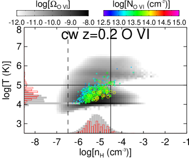
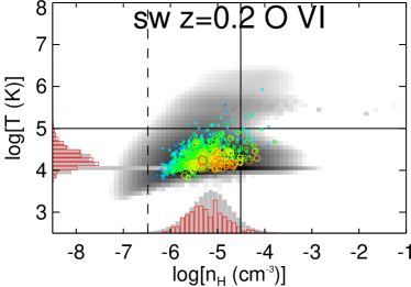
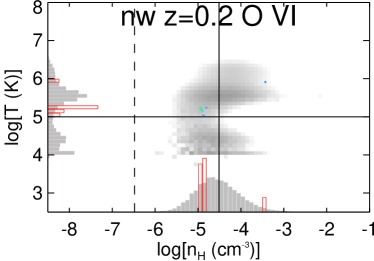
Figure 13: O vi $\Omega$ phase space diagrams as described in Figure 11 for other wind models: constant winds (cw, ${v_{\rm wind}}=680\;{\rm km}\,{\rm s}^{-1}$, $\eta=2$), slow winds (sw, ${v_{\rm wind}}=340\;{\rm km}\,{\rm s}^{-1}$, $\eta=2$), and no winds (nw) for $z=0.2$ O vi.

Overall, the conclusion that the O vi detected by COS (at least under the S/N assumptions here) will be predominantly photo-ionised is robust to variations in the wind model and the cooling rates (as we will show in §6.2). Even Ne viii, at columns just below what is currently accessible, becomes dominated by photo-ionised absorbers. Si xii at COS sensitivities probes hot gas, but not at low WHIM densities, and anyway these lines should be rare. A key conclusion from this work is that the bulk of the diffuse collisionally ionised WHIM gas, i.e. the so-called missing baryons, is only traceable through high ionisation X-ray transitions. We will explore such X-ray absorption in a forthcoming paper.

5.2 Cosmic Densities of Ions

The central theme in our exploration of the physical conditions of metal absorbers is the complex link between the enrichment patterns of metals and their observational tracers. Simulations show that even the most commonly observed low-$z$ metal absorption line, O vi, traces only a small fraction of the metals and baryons outside of galaxies (OD09; Cen & Chisari, 2011; Tepper-Garcia et al., 2011). Furthermore, even when one uses Equation 3 to sum the observed absorbers to find the cosmic density of a particular ion, $\Omega_{\rm abs}$, this does not necessarily yield the true physical mass density of that ion.

We compare the mass-weighted cosmic ion density summed via the contribution of every SPH particle outside of galaxies, $\Omega_{\rm SPH}$ (the grey shading in Figure 11) to $\Omega_{\rm abs}$ (Equation 3, the volume-weighted observational probe represented by the coloured circles for individual absorbers). Ideally the two methods should yield the same answer; i.e. $\Omega_{\rm abs}$ should recover the true $\Omega_{\rm SPH}$. We list the comparisons in Table 2 for a number of different ions and wind models along with the percentage of the $\Omega_{\rm SPH}$ recovered ($f_{\rm rec}$) in our simulated observational sample corresponding to S/N=30 COS observations over a pathlength of $\Delta z=35$ and any identified line below $10^{15}\;{\rm cm}^{-2}$. This pathlength appears to adequately sample the densities from which the species we discuss arise.

Table 2: Cosmic Densities of Ions

Ion	Redshift	Model	$\Omega_{\rm abs}^{a}$	$\Omega_{\rm SPH}^{b}$	$f_{\rm rec}^{c}$
O vi	$0-0.5$	vzw	36.7	57.6	64
”	”	cw	20.0	30.7	65
”	”	sw	41.6	65.8	63
”	”	nw	0.11	0.30	37
”	”	vzw-turb	45.9	57.6	80
C iv	$0-0.5$	vzw	11.5	34.0	34
”	”	cw	5.0	12.2	41
”	”	sw	8.5	24.2	35
”	”	vzw-turb	24.8	34.0	73
Si iv	$0-0.5$	vzw	2.3	10.3	22
”	”	cw	0.9	2.6	35
”	”	sw	1.3	5.2	25
”	”	vzw-turb	6.9	10.3	67
Ne viii	$0.5-1.0$	vzw	4.5	10.7	42
”	”	cw	4.0	8.8	45
”	”	sw	7.6	15.5	49
”	”	vzw-turb	3.4	10.7	32

^a Summed ion cosmic density by SPH particle, in units of $10^{-8}$.

^b Summed ion cosmic density by simulated absorbers, in units of $10^{-8}$.

^c Recovery percentage, i.e. $\Omega_{\rm abs}/\Omega_{\rm SPH}\times 100$.

Between 22 and 80% of $\Omega_{\rm SPH}$ is recovered, depending on the species and the wind model. Lower ionisation species often have lower $f_{\rm rec}$, which at least double for $\Omega_{\hbox{C\,{\sc iv}}}$ and $\Omega_{\hbox{Si\,{\sc iv}}}$ when turbulence is added to the vzw model. This is because these species (i) arise from higher densities that are more stochastically sampled in our sight lines, and (ii) depend heavily on the derived column densities for the strongest absorbers, from where most of the cosmic density of an ion arises. Si iv is the most stochastic absorber we follow, and arises from the highest densities ($n_{\rm H}=10^{-4}-10^{-2}\;{\rm cm}^{-3}$).

Conversely, $\Omega_{\hbox{O\,{\sc vi}}}$ and $\Omega_{{\hbox{Ne\,{\sc viii}}}}$ are higher ionisation species that trace lower densities with less stochasticity. This explains the lower dispersion of recovery fractions between the models. Recovery of $\Omega_{{\hbox{Ne\,{\sc viii}}}}$ (32-49% between $z=0.5-1.0$) suffers because of sensitivity issues; the majority of Ne viii is not well-sampled at diffuse overdensities because it is too weak to be detected. Si xii is an even more extreme example with vzw having $f_{\rm rec}=13\%$; only a portion of the collisionally ionised Si xii halo component is recovered. O vi traces a statistically well-sampled phase space with the most sensitivity to provide the most complete census of $\Omega_{\rm SPH}$, but still manages to recover at most $80\%$ of the total.

Another practical issue results from saturated absorbers that have uncertain column densities. AutoVP typically estimates lower column densities than the true value, and $\Omega_{\rm abs}$ becomes under-estimated. Adding turbulent broadening raises the column density where lines become saturated and, therefore, $\Omega_{\rm abs}$ rises and also becomes more accurate as we discuss in §6.3. This effect can be quite dramatic for species with high stochasticity such as C iv and Si iv at $z<0.5$, where applying turbulent broadening more than doubles $f_{\rm rec}$.

In summary, limited sensitivity and stochasticity can lead to inaccuracies in the determination of the cosmic ion abundance. Sensitivity issues always lead to an underestimate, while stochasticity leads to more uncertainty in an ion’s cosmic density. Additionally, saturated absorbers can hide significant amounts of true absorption, leading to under-estimates of cosmic ion densities, especially for low ionisation species. Hence while cosmic ion densities are a useful characterisation of the overall metal evolution in the IGM, detailed comparisons between models and data are more robustly accomplished using absorber statistics.

6 Model Variations

A fundamental difference between the ${\rm Ly}\alpha$ and metal-line forests is the latter’s high sensitivity to outflow models. In this section we explore such sensitivities of the model predictions to variations in some important physical and chemical assumptions. We will mainly focus on O vi, but will also consider other species. OD09 already explored a range of model variations for O vi, finding that this ion consistently traced the diffuse, $T<10^{5}$ K IGM. Given that other groups find different results for O vi (e.g. Cen & Chisari, 2011; , 2011; Tepper-Garcia et al., 2011), we concentrate our study on varying four aspects of the modelling: the ionisation background, metal-line cooling, turbulent broadening, and metal inhomogeneity. We present the EWDs and the CDDs for the variations that we explore in Figures 14 and 15, respectively, and provide cosmic O vi ion densities at $z<0.5$ in Table 3.

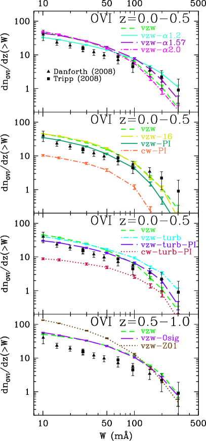
Figure 14: Equivalent width cumulative distribution plots for O vi systems at $\langle z\rangle=0.25$ for different model variations including the shape of the ionisation background (top panel, §6.1), different types of metal-line cooling (2nd, §6.2), turbulent broadening (3rd, §6.3), and the metal inhomogeneity (4th, §6.4). Models are described in the text.

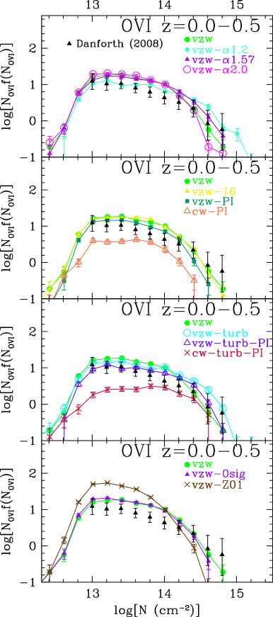
Figure 15: Column density distribution plots for O vi systems at $\langle z\rangle=0.25$ analogous to Figure 14.

6.1 Ionisation Background

Our conclusion that photo-ionisation is responsible for the majority of the absorption by high-ionisation species is sensitive to the shape and intensity of the ionisation background at far-UV and soft X-ray energies. No direct observational constraints exist between the observed slope of extreme UV (EUV) spectra of quasars (Telfer et al., 2002; , 2004) and the X-ray background (Worsley et al., 2005). The ionisation potential required to photo-ionise O vi at 8.4 Rydbergs lies in this unconstrained gap (J. M. Shull, private communication).

Table 3: Cosmic Densities of O vi between $z=0-0.5$

Model	$\Omega_{\rm abs}^{a}$	$\Omega_{\rm SPH}^{b}$	$f_{\rm rec}^{c}$
vzw	36.7	57.6	64
vzw-$\alpha 2.0$	36.2	53.4	68
vzw-$\alpha 1.57$	42.5	75.3	56
vzw-$\alpha 1.2$	41.5	110.5	38
vzw-16	37.3	56.6	66
vzw-PI	26.2	39.6	66
cw-16	23.9	35.6	67
cw-PI	7.7	11.5	67
vzw-turb	45.9	57.6	80
vzw-PI-turb	32.5	39.6	82
cw-PI-turb	11.5	11.5	100
vzw-0sig	34.4	57.6	60
vzw-Z01	51.5	71.4	72

^a Summing ion cosmic density by SPH particle, in units of $10^{-8}$.

^b Summing ion cosmic density by simulated absorbers, in units of $10^{-8}$.

^c Recovery percentage. Ratio of $\Omega_{\rm abs}/\Omega_{\rm SPH}\times 100$.

We use the CUBA package (, 2001) to generate three alternative ionisation backgrounds varying the slope of the EUV portion of the quasar spectrum. Figure 1 displays these three other backgrounds, which are referred to as HM2005 backgrounds (after Haardt & Madau 2005) with $\alpha=1.2$, 1.57, and 2.0, where the spectrum above 1 Ryd has an intensity $F_{\nu}\propto\nu^{-\alpha}$. The HM2005 background is included as an input into the latest package of CLOUDY and uses the $\alpha=1.57$ power law based on Telfer et al. (2002), but the range of slopes explored here is reasonable given the observed range and uncertainty in quasar spectral shapes (F. Haardt, private communication). The fiducial HM2001 spectrum uses $\alpha=1.8$ and is most similar to the HM2005 $\alpha=2.0$ spectrum.

The hardest background, $\alpha=1.2$, has 16 times more intensity at the O vi ionisation potential relative to the softest background, $\alpha=2.0$, while leaving the background at the Lyman limit and, therefore, the ${\rm Ly}\alpha$ forest nearly unchanged. Figure 16 shows the phase space distribution of O vi absorbers under these two extreme assumptions, and demonstrates that the peak density for $\Omega_{\hbox{O\,{\sc vi}}}$ shifts from $10^{-5.1}$ to $10^{-4.3}\;{\rm cm}^{-2}$ when moving from the softest to the hardest backgrounds (cf. grey $x$-axis histograms). However, typical O vi absorbers ($N_{\hbox{O\,{\sc vi}}}=10^{13.5-14.5}\;{\rm cm}^{-2}$) do not reflect such a dramatic shift. Recovery fractions of $\Omega_{\hbox{O\,{\sc vi}}}$ also decline from 56% to 32% (Table 3), mainly because O vi absorbers from haloes have underestimated column densities due to saturation.

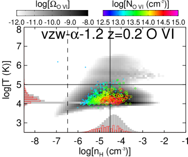
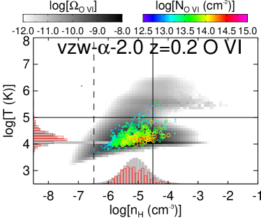
Figure 16: $\Omega$ phase space diagrams as described in Figure 11 for $z=0.2$ O vi for the two extremes in our assumed ionisation background. The top panel shows the hardest background ($\alpha=1.2$ for the EUV power law of quasars) and the softest background ($\alpha=2.0$).

The top panel of Figure 15 displays the O vi CDD for the four backgrounds. As the EUV intensity is turned up, photo-ionised O vi moves to higher overdensities creating more strong absorbers and fewer weak absorbers; a power law fit to the CDD would give a shallower slope. The $\alpha=1.2$ background model appears consistent with the EWD in the top panel of Figure 14 without the need for turbulent broadening, but the linewidths are still underestimated for strong absorbers compared to the observed $b$-parameters (not shown). When $\alpha=1.2$, strong photo-ionised O vi absorbers populate haloes while the $\alpha=2.0$ background predicts barely any photo-ionised halo absorbers. If photo-ionised O vi is clearly identified within haloes, it suggests that a hard meta-galactic ionisation background is penetrating halo gas.

Collisionally ionised O vi is a poor tracer of WHIM gas in all cases, because even the weakest ionising background efficiently photo-ionises oxygen in its collisionally ionised temperature range, peaking at $T=10^{5.45}$ K, to higher ionisation states. This is why O vi fails to trace the copious amounts of metals pushed by cw winds into the low-density $10^{5-6}$ K WHIM; this oxygen ionises to O vii and beyond. In summary, reasonable variations in the hardness of the EUV background are unlikely to alter our fundamental conclusion that most O vi absorbers detectable with COS arise in photo-ionised gas.

6.2 Metal-Line Cooling

Even if the ionisation background photo-ionises most O vi at $T>10^{5}$ K to higher states outside haloes, there still exists a potential for some O vi to trace WHIM temperatures. Cen & Chisari (2011), (2011), and Tepper-Garcia et al. (2011) all predict a significant component of collisionally ionised O vi at overdensities as low as $\sim 10$. One possible explanation is the efficiency of metal-line cooling in the $\sim 10^{5}$ K temperature regime. To explore this, we now compare two implementations of metal-line cooling– (i) the assumption of collisionally ionised equilibrium (CIE), and (ii) cooling in the presence of the (2001) photo-ionising background (PI).

Our main simulations employ the first implementation, namely that (1993) CIE metal cooling rates are added to hydrogen and helium rates calculated in the presence of the (2001) background. However, in the presence of a photo-ionising background, the number of bound electrons is reduced, leading to less efficient cooling. Tepper-Garcia et al. (2011) in their §5.3 demonstrate that photo-ionised cooling times using (2009b) rates in OWLS (OverWhelmingly Large Simulations), rates that include the effects of the UV background on the metal cooling, are significantly longer for $0.1\;{\rm Z}_{\odot}$ and $\;{\rm Z}_{\odot}$ gas at $n_{\rm H}=10^{-5}\;{\rm cm}^{-2}$. This leads to a higher equilibrium temperature where cooling balances photo-heating.

Photo-ionised rates are clearly the more physically correct cooling rates, therefore we compare the results of using our normal metal cooling implementation (adding CIE rates) to those using photo-ionised metal cooling rates based on the (2009b) solar abundance cooling tables. To do so, we evolve four $16h^{-1}{\rm Mpc}$ simulation volumes at the same resolution as our $48h^{-1}{\rm Mpc}$ simulation volumes: vzw and cw winds with CIE cooling (vzw-16, cw-16) and PI (vzw-PI, cw-PI) cooling.

We present the EWDs and CDDs for all but the cw-16 model along with the 48 $h^{-1}{\rm Mpc}$ vzw simulation in the second panels of Figures 14 and 15, respectively. The vzw-16 simulation is statistically identical to the larger vzw simulation for all O vi observations. This comes as no surprise because OD09 demonstrated that O vi is mostly associated with low-mass, $<0.3M^{*}$, galaxies, which are well sampled in both volumes. This justifies using the smaller volume to explore these physical variations.

Comparing the vzw-16 and vzw-PI simulation, there exists 70% as much O vi absorption in the latter, specifically $\Omega_{\hbox{O\,{\sc vi}}}$, $3.26\times 10^{-7}$ versus $2.35\times 10^{-7}$, with the reduction evenly distributed in column density (Figure 15, middle panel). Examination of the O vi phase space for vzw-PI in Figure 17 (upper left panel) reveals that most of the O vi absorption still arises from the diffuse O vi phase. However, there are subtle differences compared to the standard vzw model (bottom right panel). The locus of cool metals at $\delta\ga 10$ (i.e. $n_{\rm H}\ga 10^{-5.5}{\rm cm}^{-3}$) is no longer flat at $\sim 10^{4}$ K, below which CIE metal-line cooling no longer contributes, but declines from $\sim 10^{4.5}$ K to below $10^{4}$ K for increasing overdensity as seen also in OWLS (cf. Wiersma et al., 2010, their Figure 1). O vi absorbers, therefore, trace somewhat hotter temperatures, but are still within the diffuse phase. Somewhat more O vi exists in the WHIM phase owing to this less efficient cooling, but still only a handful of identified absorbers actually trace this phase.

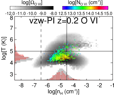
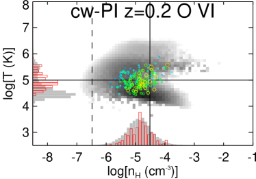
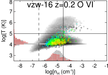
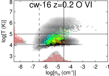
Figure 17: $\Omega$ phase space diagrams as described in Figure 11 for O vi at $z=0.2$ for simulations with photo-ionisational-dependent metal-line cooling (top panels) and the assumption of collisional ionisation for metal-line cooling (bottom panels). The left panels show the vzw models and the right panels show the cw models. We show the $16h^{-1}{\rm Mpc}$ volumes in all four cases, but the O vi observables are statistically identical to the $48h^{-1}{\rm Mpc}$ volumes for collisional ionisation cooling.

Examining the two different cooling models in the cw simulations reveals much larger differences (Figure 17, right panels); $\Omega_{\hbox{O\,{\sc vi}}}$ declines by a factor of almost three using PI cooling, from $2.08\times 10^{-7}$ to $7.1\times 10^{-8}$. The main difference is that cw winds push metals to lower overdensities where photo-ionisation plays a larger role in retarding cooling. Less oxygen cools below $10^{4.5}$ K where photo-ionised O vi ionisation fractions are the largest.

As an aside, we note that galaxy growth remains relatively unaffected by this change. The amount of stars formed at $z=0$ is reduced by only 8% using PI cooling relative to CIE cooling. This mostly arises because the reduced metal-line cooling at lower densities hinders the recycling of wind material back into galaxies (, 2010). A small reduction in overall star formation was also noted by (2011) when making the same comparison in their grid-based simulation (cf. the red and black curves in their Figure 1).

In summary, including photo-ionised cooling rates does not alter our fundamental conclusions about the phases O vi and other absorbers trace in our favoured vzw model – O vi still traces mostly diffuse, photo-ionised gas. We also demonstrate that using a different wind model (cw), similar to that used by Tepper-Garcia et al. (2011), produces a much larger change in O vi absorber properties when using photo-ionised metal cooling rates, because this model pushes many more metals into very diffuse gas where the photo-ionised cooling rates have a larger impact. We note that the vzw model does a much better job than the cw model in fitting the observed $z=0$ galactic stellar mass function below $5\times 10^{10}\;{\rm M}_{\odot}$ (, 2010), from which most O vi absorption arises (OD09). Hence, we favour the vzw model, although our tests do illustrate that the interpretation of observed O vi still could depend on the details of the input physics.

6.3 Turbulent Broadening

In OD09 we introduced a heuristic prescription to add sub-grid turbulent broadening to the $b$-parameters of O vi, after the conclusion of the simulation, using specexbin. This added turbulent broadening is a function of the physical density of the gas. The prescription adds an additional turbulent $b$-parameter in quadrature where

$$b_{\rm turb}=\sqrt{1405{\rm log}[n_{\rm H}]^{2}+15674{\rm log}[n_{\rm H}]+43610}~{}\;{\rm km}\,{\rm s}^{-1},$$ (4)

over the range $n_{\rm H}=10^{-5.31}$ to $10^{-4.5}\;{\rm cm}^{-3}$ and

$$b_{\rm turb}=13.93\log(n_{\rm H})+101.8~{}\;{\rm km}\,{\rm s}^{-1}$$ (5)

over the range $n_{\rm H}=10^{-4.5}$ to $10^{-3.0}\;{\rm cm}^{-3}$. Furthermore, $b_{\rm turb}$ retains its maximum value of $60\;{\rm km}\,{\rm s}^{-1}$ at higher densities. See OD09 §4.4 for an in-depth discussion of the physical motivation for this model and its relation to the turbulence observed on kpc scales in C iv paired absorbers along lensed quasar sight lines at $z\sim 2-3$ (, 2001). OD09 argue that the turbulence is related to outflows and decays on timescales of the order of a Hubble time.

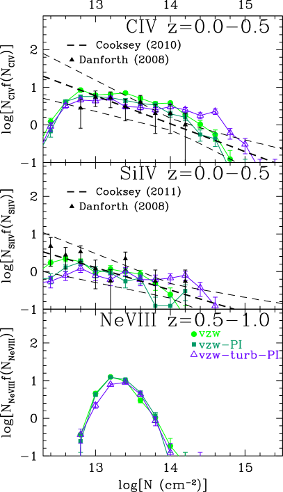
Figure 18: Column density distribution plots for C iv, Si iv, and Ne viii for vzw winds with photo-ionisation-dependent cooling rates and turbulent broadening. Error bars correspond to Poisson errors.

We already showed results for the vzw-turb model in Figures 6 through 10. Here we combine it with the vzw and cw models with photo-ionised cooling rate (vzw-turb-PI, cw-turb-PI) shown in the third panels of Figures 14 and 15. Photo-ionised metal-line cooling rates reduce vzw O vi line frequencies and $\Omega_{\hbox{O\,{\sc vi}}}$ by the same factor, one-third, either including turbulence or without it. The vzw-turb-PI model agrees well with the observed O vi CDD and EWD, and better than the vzw-turb model, which over-produces weak O vi absorbers. The vzw-turb-PI model is our favoured model for O vi as it has the most physically motivated combination of outflows, ionisation background, physical metal-line cooling, and turbulent broadening to explain both O vi and ${\rm Ly}\alpha$ forest observations (D10), as well as other observations of low-$z$ galaxies (, 2010; Davé et al., 2011a, b).

We show the C iv, Si iv, and Ne viii CDDs for this model along with the vzw-PI model in Figure 18. As before, our favoured model continues to overproduce the incidence of the lower-ionisation species. We do not believe this discrepancy can be mitigated by cosmic variance, because even our $16h^{-1}{\rm Mpc}$ box is sufficient to sample the gas and galaxies responsible for the absorption of these ions (cf. vzw and vzw-16 show nearly identical results). However, the idea of adding turbulent broadening for lower ionisation species that trace higher densities may not be as valid as in the case of O vi. For instance, using lensed quasars probing the $z\sim 2.3$ IGM, (2007) observed sub-kpc sub-structure in lower ionisation species including C iv and Si iv that did not exist in O vi. At low redshifts, all of the Si iv and most of the C iv in our models have densities where our turbulence model predicts $b_{\rm turb}>40\;{\rm km}\,{\rm s}^{-1}$, but the observations of C iv suggest much narrower linewidths (e.g. , 2010). Hence O vi may be tracing more diffusely distributed gas that is more affected by large-scale turbulence injected by outflows, while C iv and Si iv could be tracing individual high-density cloudlets. Regardless, models both with and without turbulence overpredict the C iv and Si iv absorption.

Figure 19 shows the phase-space diagram for metals and absorbers in the vzw-turb-PI model. Si iv and stronger C iv absorbers trace much higher densities than O vi. This results in many more strong C iv and Si iv components than in the vzw-PI model, because AutoVP finds stronger $N$s for otherwise non-broadened saturated profiles and weaker absorbers are subsumed into the stronger ones. The histograms in Figure 19 show that these absorbers mostly arise in cool halo gas. A difficulty with our simulations is that we may not resolve cooling instabilities in the halo gas (e.g. , 2004) that could result in much of the carbon being in dense cold cloudlets, which would favour lower ionisation states than C iv. This is in principle easily possible as only 3-5% of the carbon outside of galaxies resides in C iv between $z=0-0.5$ (vs. 13-15% at $z=2-4$), and hence a small change in the ionisation rate at $\sim 3-4$ Ryd could dramatically change the C iv statistics. It will be interesting to compare our predictions of C ii and C iii to observations when a sufficient sample becomes available, to see if we significantly underpredict the amount of carbon in these states corresponding to our overprediction of C iv.

Another possibility is that the (2004) Type II carbon yields we use are too high. For example, the (1995) carbon yields are $\sim 0.2$ dex lower, which could explain some of the differences with respect to the observations. The AGB stellar yields we use cannot explain the over-estimate, because carbon production from AGB stars is sub-dominant to Type II SNe in our simulations (, 2008). Yet another potential explanation is that a substantial fraction of carbon and silicon are depleted onto dust, while the more volatile oxygen is not. Zu et al. (2011) find that the vzw model can explain the observational evidence for intergalactic dust (Ménard et al., 2010) if the IGM dust-to-gas ratio is about half that in the Milky Way ISM, which about 25% of intergalactic metals (by mass) in dust.

Ne viii traces similar overdensities as O vi and hence should be affected by the same turbulence, and hence the vzw-turb-PI model should be the most appropriate. But as Figure 18 shows, the predicted column density distributions do not vary significantly with PI cooling or turbulence. In detail, between $z=0.5-1.0$, $\Omega_{{\hbox{Ne\,{\sc viii}}}}$ slightly increases with PI cooling, but declines by a factor of 20% with the addition of turbulence to $4.0\times 10^{-8}$, because already weak lines are broadened enough so that AutoVP fails to identify them. Most of the Ne viii absorption still traces photo-ionised gas, but the reduced cooling raises the bulk of Ne viii absorbers from $T=10^{4.0-4.4}$ K to $10^{4.4-4.9}$ K and leads to 22% compared to 7% of the Ne viii absorption arising from $T>10^{5}$ K gas (Figure 19). This percentage could grow even larger if our simulations adequately resolved interfaces between cool and hot gas within haloes, which they do not as we discussed in §5.1.

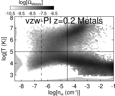
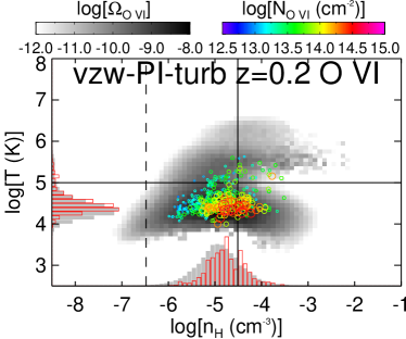
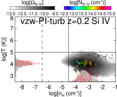
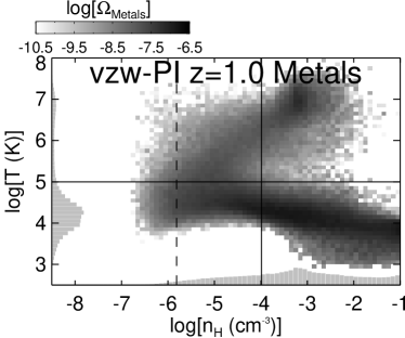
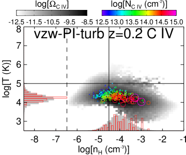
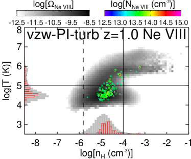
Figure 19: $\Omega$ phase space diagrams of the vzw-turb-PI model for metals, Si iv, C iv, and O vi at $z=0.2$; plus metals and Ne viii at $z=1$.

We show the cw-turb-PI model to demonstrate that turbulent broadening affects other wind models in much the same way as the vzw model, by making more wide O vi absorbers and slightly fewer weak absorbers (cf. cw-PI model). This more appropriate cooling rates applied to the cw model, combined with turbulent broadening to match observed line widths indicates this model far under-produces O vi, especially weaker systems, when compared to observed EWDs and CDDs.

6.4 Metal Inhomogeneity

The degree of metal inhomogeneity in the IGM remains highly uncertain, but dynamically very important. The distribution of metals affects gas cooling, which is critical for galaxy formation because the temperature of the gas determines the efficiency of gas accretion onto galaxies (, 2003, 2005, 2006, 2009). More metal mixing leads to more star formation as more efficient metal-line cooling affects more baryons (, 2009a). In our simulations, we do not mix metals, and each wind particle retains its own metals as it propagates out of galaxies.

The homogeneity of metals impacts the statistics of absorbers, which we explore here. We consider two ad hoc models for distributing metals throughout the IGM, by replacing particle metallicities in our simulation with prescriptive metallicities in our vzw model. In the first (vzw-Z01), we assume a uniform metallicity of $0.096\;{\rm Z}_{\odot}$ in the IGM (vzw-Z01), which is the global $z=0$ IGM metallicity in our vzw model. Note that this is similar to $0.1\;{\rm Z}_{\odot}$ painted onto earlier simulations to reproduce older observed O vi absorber frequencies (, 2001, 2001, 2003). The second model (vzw-0sig) takes the average [O/H] of the vzw model in each $0.1\times 0.1$ dex pixel of phase space (upper left panel of Figure 20 at $z=0.25$) and paints this metallicity onto all SPH particles within that phase space cell, with zero dispersion. Both prescriptions preserve the total metal mass, but neither model is dynamically self-consistent, because metal cooling would alter the physical state of the gas and feedback would have to enrich the baryons in the first place. However, our purpose here is to explore extreme cases of metal homogeneity to see if absorption line statistics can distinguish the level of metal inhomogeneity.

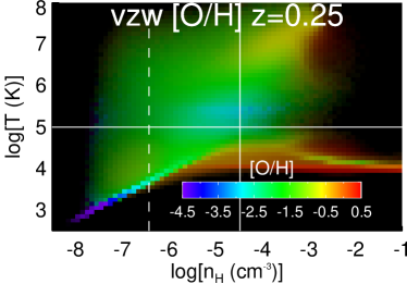
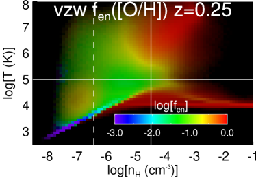
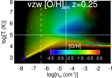
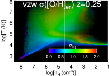
Figure 20: Phase space diagrams displaying oxygen metallicity characteristics for the r48n348vzw simulation at $z=0.25$. The colour scales correspond to mean metallicity (upper left), the fraction of baryons enriched to at least $10^{-6}\;{\rm Z}_{\odot}$ (upper right), the median metallicity of the enriched fraction (bottom left), and the log-normal metallicity dispersion of the enriched fraction (bottom right).

Figures 14 and 15, bottom panels, show the EWDs and the CDDs of these models, compared to our original vzw model. The vzw-Z01 model, as found in OD09, produces too many weak absorbers, too few strong absorbers (in terms of column density), and a large alignment fraction with H i (Figure 21). Collisionally ionised O vi ($T>10^{5}$ K) accounts for a quarter of $\Omega_{\hbox{O\,{\sc vi}}}$ and two-thirds of lines above $N_{\hbox{O\,{\sc vi}}}>10^{14}\;{\rm cm}^{-2}$. Simply painting metals onto a simulation uniformly overestimates O vi and other species in CIE, because the most commonly observed UV resonance lines (C iv, O vi, and soon Ne viii) are also some of the most important coolants.

Painting the average metallicity by phase space pixels explores how the dispersion in metallicity among SPH particles affects the line statistics. This model shows negligible differences versus the original vzw case, showing that the fact that metals are not mixed in our simulations has no impact on O vi absorber statistics. We reiterate that this test does not dynamically account for differences in the cooling rates that would result from such metal mixing, and hence it is not self-consistent; this test isolates the impact of spatial inhomogeneities in the metals.

Figure 20 provides a broader view of metal inhomogeneity in our original vzw simulation. The upper left shows the oxygen metallicity in phase space, this is similar to Figure 2 except here we only consider oxygen and the general trends are as before. The upper right panel shows the fraction of baryons enriched with oxygen, $f_{\rm en}$, using a threshold of [O/H]=$10^{-6}\;{\rm Z}_{\odot}$. $f_{\rm en}$ is not very sensitive to this threshold and is used to discard SPH particles enriched to very low levels by delayed feedback. Practically all the ICM gas and most gas, both hot and cold, inside of haloes is enriched. Interestingly, the $f_{\rm en}$ distribution for the nw simulation (not shown) looks nearly identical to the vzw model above $10^{5}$ K, indicating that enrichment mechanisms other than outflows (e.g. dynamical stripping, delayed feedback) are getting hot baryons, i.e. hot halo and WHIM gas, above this threshold metallicity. In the IGM outside of haloes, most particles remain pristine, as the typical fractions of enriched particles are $\la 0.1$. In photo-ionised gas within voids, the fraction of enriched particles can drop below $10^{-3}$.

The lower left panel shows the average metallicity of only the enriched particles, [O/H]_en. This demonstrates that much of the enriched portion of the diffuse IGM has [O/H]=$0.1-0.3\;{\rm Z}_{\odot}$. Since the outflows carry out metals that are representative of the ejecting galaxy, this indicates that the dominant galaxies enriching the IGM tend to have sub-solar metallicities; these galaxies are generally well below $L^{*}$ (as found in , 2008). However, there is a selection effect that highly enriched IGM particles undergo stronger metal-line cooling, dropping them out of the warmer phases onto the photo-ionised locus. Hence enriched particles in the underdense regions actually have higher metallicities than the WHIM gas in moderately overdense regions, since these are the only particles that can cool at such low densities. Nevertheless, the $f_{\rm en}$ shows that such particles are quite rare.

The lower right panel shows the log-normal dispersion, $\sigma$([O/H]_en) of the metals around the median log[[O/H]_en] for the enriched particles only. Both (2003) and (2004) found that C iv and O vi enrichment at $z\sim 2-4$ could be described by a log-normal distribution, but applied to all baryons. In general, regions with dispersions below 0.5$\sigma$ are enriched via outflows consisting of ISM gas having similar metallicities. The higher dispersions correspond to regions enriched via other mechanisms such as dynamical stripping and delayed feedback from intracluster stars.

6.5 Alignment Statistics

The association of H i with O vi offers a potentially powerful way to explore metal inhomogeneity. We show alignment statistics of O vi components with nearby H i components in Figure 21. We plot the fraction of O vi absorbers with an associated H i absorber at or below the velocity difference indicated on the $x$-axis, with the criteria that both absorbers have $W\geq 30$ mÅ and $z<0.5$. Overlaid are STIS data from (2008) using the same selection criterion.

The data are unable to discriminate between vzw and vzw-0sig, but disfavour the vzw-Z01 model, which tends to produce more alignment. OD09 showed that O vi absorbers trace similar diffuse densities and temperatures as H i, but that the O vi-traced enriched gas is inhomogeneous and clumpier than the diffuse baryons traced by the ${\rm Ly}\alpha$ forest. The difference in metal inhomogeneity between the vzw and vzw-0sig models does not show up in the EWD and CDD distributions in Figures 14 and 15, but the expected observational sample of the two most common species probed by COS is expected to provide the ability to statistically distinguish these two models. The cw model shows lower alignment owing to faster winds pushing metals further from the ${\rm Ly}\alpha$ in both physical and velocity space. Both turbulence and photo-ionisation-dependent cooling (not shown) do not alter the statistics from the vzw model.

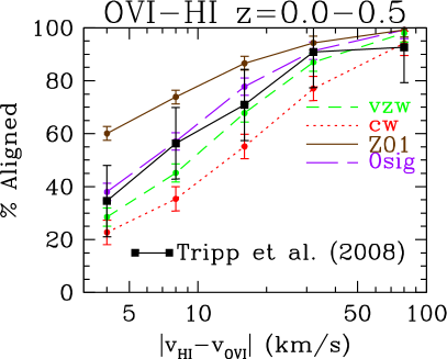
Figure 21: Alignment fractions for O vi with H i components between $z=0-0.5$ as a function of inter-species component velocity difference. Both O vi 1032Å and H i 1216Å are required to have $W>30$ mÅ.

Alignment statistics versus H i fundamentally probe the level of photo-ionisation in metal absorption, because H i arises almost exclusively in photo-ionised gas. Models that produce more collisionally ionised O vi will therefore have significantly less alignment with H i. Current observations of O vi-H i alignment from (2008) shown in Figure 21 suggest that the vzw model produces roughly the correct level of photo-ionised gas in relation to H i, and therefore strongly favours our conjecture that much of the O vi seen with COS is photo-ionised.

7 Discussion

Our favoured model includes momentum-conserved winds and uses photo-ionisation-dependent cooling rates. The vzw-turb-PI model matches the O vi statistics including the $z<0.5$ EWD, CDD, $\Omega_{\hbox{O\,{\sc vi}}}$, and $b$-parameters when turbulent broadening is added as argued and theoretically motivated in OD09. We further advocate vzw winds for their ability to provide an adequate fit to the $z=0$ galactic stellar mass function below $5\times 10^{10}\;{\rm M}_{\odot}$ (, 2010), from which most O vi absorption arises (OD09), as well as other properties of the low-redshift galaxy population (Davé et al., 2011a, b); these galaxy properties are not expected to be greatly impacted by adding IGM turbulence or PI cooling. The HM2001 ionisation background multiplied by 1.5 appears capable of both reproducing the observed ${\rm Ly}\alpha$ forest (D10) and O vi that is principally photo-ionised. The vzw wind model also has successes fitting higher redshift data, including the $z=2$ mass-metallicity relationship (, 2008), the $z\geq 6$ galaxy luminosity function (, 2006, 2010), and observations of IGM metal enrichment at redshifts $\geq 1.5$ (, 2006, 2009). The most obvious failing of the vzw model is its inability to quench star formation in $\ga M^{*}$ galaxies and create the observed red sequence, although this likely has to do with our simulations lacking a mass-dependent quenching mechanism such as AGN feedback (, 2010, 2011). However, massive galaxies are not responsible for the vast majority of O vi enrichment (OD09), because they enrich a comparatively small volume of the Universe, and so this quenching of massive galaxies is not expected to significantly impact our IGM enrichment levels.

Nevertheless, this model also has significant problems that are shared by the other wind models we consider here. C iv and Si iv observations pose a problem in that our favoured model produces too many absorbers compared to (2010, 2011). It might be possible to alter the ionisation background at 3-4 Rydbergs to mitigate this discrepancy while still satisfying the other observational constraints. Updated ionisation backgrounds generated with the new version of CUBA (Haardt & Madau, 2011) are worth exploring in the future. Alternatively, our assumed yields could be too high, or carbon and silicon could be preferentially depleted onto dust (Zu et al., 2011). However, the discrepancy may result from limitations present in our simulations, namely that we fail to resolve cooling instabilities in halo gas where such lower-ionisation absorbers are expected to arise. Quantifying C ii and C iii absorption may help distinguish between these possibilities. Our favoured model also under-predicts the frequency of Ne viii lines with column densities similar to those observed so far (Narayanan et al., 2009), which again may be a result of insufficient resolution within the halo gas, in the sense that we fail to resolve metal-bearing interfaces between cold clumps embedded in hot, tenuous halo gas. Relatedly, OD09 (§5.4) found a lower frequency of complex, collisionally ionised O vi absorbers, which may also arise in shock interfaces within hot halo gas, as implied by some observations.

In contrast, absorbers arising in more diffuse gas should be more robustly modelled in our simulations. Hence, we are confident that, when probed to sufficiently low column densities, most high ionisation lines of O vi and Ne viii will mostly trace diffuse photo-ionised gas. Since there have been a number of recent publications exploring O vi and other metal-line statistics in cosmological simulations to $z=0$, we now compare and contrast our results with these works.

7.1 Feedback Methods in Other Simulations

Our discussion of alternative feedback methods begins with Cen & Chisari (2011), who generate statistics for O vi and C iv from $z=6\rightarrow 0$ in a 50 $h^{-1}{\rm Mpc}$ $2048^{3}$-cell uniform mesh simulation. Their winds are implemented by distributing gas and energy onto the 27 nearest cells (, 2005), which instantaneously distributes metals over a 73 comoving $h^{-1}{\rm kpc}$ cube. Clearly this model does not self-consistently track the dynamics of enriching this cube, but it nevertheless provides a heuristic way to distribute metals into the IGM. Their favoured wind efficiency is $\epsilon_{\rm GSW}=7\times 10^{-6}$, where $\epsilon_{\rm GSW}$ represents the fractional rest mass energy of all stars formed put into thermal feedback. Their total wind energy is then $E_{\rm wind}=1.2\times 10^{49}$ erg/$\;{\rm M}_{\odot}$, which Cen & Chisari (2011) argue is roughly comparable to the total SNe energy in a Chabrier initial mass function (IMF).

(2011) similarly use fixed-mesh Eulerian simulations and parametrise star formation and feedback the same way. They can reproduce much of the observed $z<0.4$ O vi CDD with a wind energy efficiency of $\epsilon_{\rm GSW}=10^{-5}$. We calculate their total $E_{\rm wind}=1.8\times 10^{49}$ erg/$\;{\rm M}_{\odot}$, which is nearly twice the SNe energy available in a Chabrier IMF if all stars $\geq 10\;{\rm M}_{\odot}$ explode as $10^{51}$ erg SNe, but about equivalent if all stars $\geq 6\;{\rm M}_{\odot}$ explode as SNe. (2011) advocate the need of distributing feedback over 27 cells (as in Cen & Chisari 2011) to fit the observed star formation rate density history, whereas limiting the feedback to one cell makes it much less efficient at curtailing star formation. This means that in their case, metals are instantaneously distributed over a 99 to 294 $h^{-1}{\rm kpc}$ cube depending on their simulations.

Our simulations, in contrast, attempt to directly mimic observations of galaxies that indicate wind speeds of hundreds of km/s emanating from galaxies (e.g. Steidel et al., 2010), and scaling with the circular velocity (e.g. , 2005a). We are inevitably limited by resolution and numerics in that we cannot fully resolve how winds escape from galaxies, so we are forced to employ parametrisations for these winds. The adopted parametrisations (including hydrodynamic decoupling) are intended to represent observed winds at the scales at which they are observed. It is interesting that our winds typically travel $\sim 100$ physical kpc (, 2008), which is similar to the scales over which Cen & Chisari (2011) and (2011) assume outflows distribute gas. The difference is that some of our winds can travel much farther or not as far, depending on the self-consistently tracked interaction between the gas and the ambient medium; we do not directly parametrise how far winds and metals travel. Moreover, in these fixed mesh simulations the distance metals travel is explicitly governed by the spatial resolution, while in our case the wind speeds are based on the galaxy mass, which is a well-converged quantity. For instance, the lower-resolution mesh simulations of (2006) produce a significant O vi signal without any mechanism for distributing gas to nearby cells, in contrast to our no-wind case that produces essentially no IGM metal absorbers. The direct sensitivity of fixed mesh simulations to ad hoc numerical parameters makes it difficult to interpret their conclusions about the physics driving IGM enrichment. Adaptive mesh refinement (AMR) simulations could potentially provide a less resolution-sensitive implementation of winds.

Finally, we point out that our feedback model has quite modest energy requirements relative to the above mesh simulations. Both (2011) and Cen & Chisari (2011) strain the limits of available supernova energy. Our cw model and the feedback prescription in Tepper-Garcia et al. (2011) (${v_{\rm wind}}=600\;{\rm km}\,{\rm s}^{-1}$, $\eta=2$) require substantial fractions of SN energy to be converted directly to kinetic winds– $E_{\rm wind}/E_{\rm SN}=0.75-0.97$ assuming the (conservative) $10\;{\rm M}_{\odot}$ lower mass limit for SNe. Comparatively, the vzw model has $E_{\rm wind}/E_{\rm SN}=0.56$ at $z=1$ and $0.45$ at $z=0$, which is meant as an illustrative comparison since this wind prescription simulates energy generated during the lifetimes of O and B stars. Because vzw feedback energy scales with $\sigma$, the lower mass galaxies that are primarily responsible for the enrichment of the diffuse IGM have even less of an energy requirement. For instance, a $M_{*}=10^{10}\;{\rm M}_{\odot}$ galaxy has $E_{\rm wind}/E_{\rm SN}=0.30$ at $z=1$ and 0.21 at $z=0$. Note that (2009) in their §5.4 misinterpret the vzw model as requiring more energy than in the SN energy budget; this is true only for central galaxies in haloes more massive than $10^{13.5}\;{\rm M}_{\odot}$ at $z=1$, or for between 2-4% of all wind particles launched at any redshift. These galaxies are not responsible for enriching the IGM, and in any case should not have significant ongoing star formation today (, 2010).

7.2 Metal Mixing

Absent in our simulations is any attempt to simulate the mixing of metals. For the purposes of cooling and generating mock spectra, we use particle metallicities, which is in contrast to Tepper-Garcia et al. (2011), who smooth metallicities over SPH particle smoothing lengths when calculating metal-line cooling. Their metal smoothing was introduced in (2009a), who calculate that smoothed metallicities are $\sim 2/9$th the individual particle metallicities when all surrounding particles in their kernel are pristine. Given that our metal-enriched IGM wind particles are often surrounded by pristine gas, the cooling times of our metals could be as much as $\sim 4.5$ times shorter using our individual particle metallicities if metal-line cooling dominates total cooling. We suggest this could be the source of the greatest differences with the results of Tepper-Garcia et al. (2011), who find the majority of O vi above $10^{5}$ K. Our cw-PI model is most similar to their “REFERENCE” model with notable other differences including a slightly higher wind speed (${v_{\rm wind}}=680$ vs. $600\;{\rm km}\,{\rm s}^{-1}$) and that we decouple our winds; both of these should make it easier for winds to escape galaxies in our simulations. Nonetheless, both simulations have similar $\Omega_{\hbox{O\,{\sc vi}}}$ and similar overdensities bearing O vi gas, but most of our O vi gas resides around $10^{4.5}$ K, whereas theirs is at $10^{4.8-5.5}$ K with significantly more O vi at temperatures $>10^{5.1}$ K.

Fixed mesh simulations with distributed feedback also can lead to much smoother metallicities, resulting in longer cooling times and hotter metal-bearing gas. We argue that the lack of metal smoothing is a fundamental difference causing a significant photo-ionised component of O vi in our simulations versus others (Cen & Chisari, 2011; , 2011; Tepper-Garcia et al., 2011). Both Tepper-Garcia et al. (2011) and (2011) make a strong case that using CIE metal-line cooling rates over-estimates cooling resulting in too much photo-ionised O vi in OD09. This is no doubt true, especially given the fact that in our cw simulations, photo-ionised metal-line cooling rates reduce $\Omega_{\hbox{O\,{\sc vi}}}$ by a factor of three. But as we demonstrated in §6.2, for our favoured vzw case the difference is much less. Still, metal mixing can be an important determinant for the IGM phase of O vi absorbers.

Treatments of metal diffusion have been implemented into other simulations (, 2009, 2010), but it remains unclear to what extent metals mix in the IGM. Interpreting observations of metal absorbers at higher redshift suggest that metals could remain in concentrated, small cloudlets with metallicities similar to galactic ISM gas (, 2006, 2007). This scenario would favour our lack of mixing and the fact that winds carry ISM gas directly into haloes and the IGM. In summary, the necessity and specific implementation of metal mixing remains uncertain when considering the low-$z$ IGM. It appears that metal mixing is as determinative as implementations of metal-line cooling or feedback for interpreting IGM metal-line observations.

8 Conclusions

We examine the absorption and physical conditions of metals residing in the $\sim$90% of baryons outside of galaxies between $z=0$ and $2$. We employ $48h^{-1}{\rm Mpc}$, $2\times 384^{3}$-particle cosmological simulations, the same simulations used by (2010) to explore the $z=0$ galactic stellar mass function and by Davé et al. (2010) to explore the ${\rm Ly}\alpha$ forest. Our work builds on the previous results of (2009), finding fundamentally the same conclusions for O vi, and also makes predictions for Si iv, C iv, Ne viii, Mg x, and Si xii specifically tailored to the expected instrumental characteristics of the Cosmic Origins Spectrograph (COS). We subdivide the gas phases between the true IGM ($\delta<120$ at $z=0$) and gas within dark matter haloes ($120<\delta<10^{5.7}$ at $z=0$), and between hot ($T\geq 10^{5}$ K, WHIM and hot halo) and cool ($T<10^{5}$ K, diffuse and condensed) phases.

Metal-line absorption is fundamentally different than its primordial big brother, the ${\rm Ly}\alpha$ forest, owing to its much greater sensitivity to the processes of galaxy formation and evolution. While galactic outflows suppress star formation and therefore metal production, they concurrently distribute metals into haloes and the IGM. Our simulation without winds (nw) produces 2.1 times more metals by $z=0$ than the momentum-conserved wind (vzw) model, but the vzw simulation has 3.5 times more gaseous metals outside of galaxies, and 380 times more metals in the diffuse IGM phase from which most IGM metal absorbers arise. The resulting enrichment patterns are quite sensitive to the details of the enriching outflows. The combination of wind velocities and environment determines to how low a density the winds reach, e.g., whether or not metals leave their dark matter haloes. Low velocities from dwarf galaxies easily reach the IGM, while $>1000\;{\rm km}\,{\rm s}^{-1}$ winds from $>M_{*}$ galaxies often fail to escape their haloes because of the greater ambient density of the surrounding gas (, 2010). The wind velocity also determines the temperature to which the gas shock heats as the wind decelerates. Fast winds that shock gas to $\ga 10^{6}$ K are more likely to join the WHIM or hot halo gas. The density and temperature where the metals are deposited in turn impacts their cooling rate, which can return enriched gas to photo-ionisation temperatures. Tracking all these processes dynamically within growing large-scale structure presents a complex and challenging problem that impacts our understanding of a wide range of phenomena related to the cosmic evolution of baryons.

Our main results are as follows:

$\bullet$ Metals progressively are found in more overdense regions from $z=2\rightarrow 0$. By $z=0$ in our favoured momentum-conserved wind (vzw) model, only 4% of metals are outside of haloes (i.e. at densities below the threshold defined by Equation 1), compared with $20\%$ at $z=2$. The constant wind (cw) model has many more metals outside of haloes, but they mostly reside in the difficult-to-detect WHIM phase. The majority of metals today reside within galaxies, in contrast to the bulk of baryons that reside outside of haloes (§3).

$\bullet$ For all the wind models, the mean metallicity of most of the baryonic phases is very slowly rising since $z\sim 2$. The exception is the condensed phase, which shows a more rapid rise as winds progressively enrich halo gas closer to galaxies at later epochs. By $z=0$, the IGM metallicities in both the cool (diffuse) and the hot (WHIM) phases are $\sim 1/50\;{\rm Z}_{\odot}$ in the vzw model, and $\bar{Z}=0.096\;{\rm Z}_{\odot}$ in the 90% of baryons outside galaxies (§3).

$\bullet$ The IGM is enriched in an “outside-in” fashion where lower overdensities are enriched at higher redshift. Higher ionisation metal species generally trace older metals at lower overdensities owing to these species being primarily photo-ionised. The ${v_{\rm wind}}\propto\sigma$ relation for vzw outflows results in a continuously rising metallicity-overdensity gradient and a gradual age-overdensity anti-correlation, which contrasts with the constant wind simulations (§3.3).

$\bullet$ Constant (cw), momentum-conserved (vzw), and slow (sw) wind models all predict $z<0.5$ O vi observational statistics (equivalent width distributions, column density distribution, cosmic ion densities) that agree within a factor of two with observations by STIS and FUSE. By contrast, the no-wind model produces an O vi incidence 100 times lower than the other feedback models and observations, which strongly emphasises the need for galactic superwinds to enrich the IGM to the observed levels. All wind models over-produce the C iv and Si iv incidence relative to available observations (§4).

$\bullet$ O vi, C iv, and Si iv absorbers predominantly (by number) arise in photo-ionised, cool gas. Photo-ionisation results in higher ionisation lines tracing lower gas densities: Si iv and C iv arise primarily from halo gas at $z<0.5$, while O vi arises mainly in the diffuse IGM (§4,5.1). We predict a population of Ne viii absorbers with $N_{{\hbox{Ne\,{\sc viii}}}}\la 10^{13.6}\;{\rm cm}^{-2}$ tracing photo-ionised diffuse $T<10^{5}$ K gas at overdensities of $\sim 10$. Stronger Ne viii absorbers (like stronger O vi systems) are more likely to be associated with $T=10^{5.5-6.0}$ K gas and may share more in common with the absorbers already detected (§4,5.1). These results do not change when using metal-line cooling rates including the presence of a photo-ionising background (§6.2,6.3).

$\bullet$ Mg x and Si xii absorbers are very rare, with frequencies of $dn/dz<<1$ for COS S/N=30 spectra in all of our models. These absorbers likely trace halo gas at $T>10^{6}$ K (§4,5.1). These species and Ne viii all have a significant photo-ionised component, which is consistent with the shape of the (2001) ionisation background; however Mg x and Si xii are too weak in this state to be detected using COS (§5.1.1). No UV tracer we examine consistently and predominantly traces WHIM gas, i.e. shock-heated gas outside of galaxy haloes.

$\bullet$ Using metal-line cooling rates accounting for photo-ionisation by the ionisation background (, 2009b) reduces the incidence of O vi absorbers at all column densities by one-third in the vzw model, which still provides an acceptable match with the observations. The difference is more dramatic for cw winds since it pushes metals to lower overdensities; O vi statistics are reduced by two-thirds and arise from gas closer to $T=10^{5}$ K. Tepper-Garcia et al. (2011) and (2011) correctly argue that assuming collisional ionisation equilibrium for metal cooling rates (with no photo-ionisation) leads to over-efficient metal-line cooling; however we find that the moderate vzw winds leave metals at higher overdensities where metal-line cooling is still efficient even in the presence of photo-ionisation and results in most of the O vi absorbers tracing $T<10^{5}$ K gas (§6.2).

$\bullet$ We reiterate the result of OD09 that heuristic turbulent broadening is required to reproduce the observed O vi linewidths, but we suggest that this prescription may not be applicable to C iv and Si iv primarily arising from haloes. O vi arises from longer columns with potentially many cloudlets with random/turbulent velocities at sub-particle scales, while lower ionisation species are more likely to trace individual higher density cloudlets (§6.3).

$\bullet$ Absorber alignment statistics of H i with O vi provide an independent constraint on the level of metal inhomogeneity in the IGM, which we quantify in §6.4. We disfavour a uniform metallicity of $Z=0.1\;{\rm Z}_{\odot}$ from comparisons with existing data, and future COS observations can potentially quantify the fraction of enriched gas and the dispersion of metals in the IGM (§6.5).

$\bullet$ The metal-line statistics to be probed by COS rarely vary by a factor of more than two between the different feedback models, despite enrichment patterns varying by much greater factors (e.g., 6.4 times more metals in the $z=0$ WHIM of cw vs. vzw). The relatively restricted density-temperature phase space traced by O vi, C iv, Si iv, and Ne viii are enriched similarly in all wind models relative to the total distribution of metals outside galaxies (§3.2,5.1.2).

$\bullet$ The observed cosmic ion density $\Omega$ summed from absorbers typically underestimates the total $\Omega$ of an ion. The stochastic effects of high overdensities being probed rarely in a volume-averaged measurement plus a large fraction of an ion’s cosmic density being contained in saturated lines make accurate determinations of $\Omega_{\hbox{C\,{\sc iv}}}$ and $\Omega_{\hbox{Si\,{\sc iv}}}$ more difficult. We estimate recovery fractions of 56-69% for $\Omega_{\hbox{O\,{\sc vi}}}$ and 30-39% for $\Omega_{{\hbox{Ne\,{\sc viii}}}}$ in S/N=30 COS observations. These fractions may be sensitive to the quality of the spectra and the fitting method used to estimate the column densities (§5.2).

$\bullet$ Exploring alternative ionisation backgrounds given the observed range of quasar emission slopes beyond the Lyman limit, we find that the slope of the O vi column density distribution becomes shallower using a harder background. The ionisation background strength varies by a factor of 16 at the O vi photo-ionisation edge (8.4 Rydberg), but even for the weakest field O vi remains primarily photo-ionised. Slopes of $\alpha=1.57$ and harder predict more photo-ionised O vi arising from halo gas (§6.1).

While metal lines observed by COS are more sensitive to the processes regulating galaxy evolution, they are also more uncertain in their modelling and interpretation compared to the ${\rm Ly}\alpha$ forest. Our parameter exploration finds good fits to existing O vi statistics, but appears to over-produce C iv and possibly under-produce Ne viii arising in hot haloes. Like OD09, we favour a momentum-conserved wind model with turbulent broadening, although we note that metal-line cooling in the presence of the photo-ionising background reduces O vi by a third and makes the average absorber hotter (30,000 vs. 15,000 K); however our O vi results are still consistent with the current data. We further advocate this model for its ability to reproduce the galactic stellar mass function below $M=5\times 10^{10}\;{\rm M}_{\odot}$ (, 2010), which are the same galaxies that are primarily responsible for IGM enrichment (OD09).

We double down on our prediction of a primarily photo-ionised origin for most UV absorbers (OD09), but realise the risky nature of our gamble. Our model variations show just how sensitive metal-line statistics are to the shape of the ionisation background at poorly constrained energies, the stiff behaviour of metal-line cooling, and a turbulence model that is surely over-simplified. How metals mix in haloes and the IGM is perhaps the most under-appreciated uncertainty for simulating such observations. Our scheme of launching ISM gas with no mixing may be the largest difference with other works with smoother metallicities leading to hotter temperatures (Cen & Chisari, 2011; , 2011; Tepper-Garcia et al., 2011); however, there is observational evidence and theoretical motivation that small, highly-enriched cloudlets remain un-mixed in the IGM (, 2006, 2007). The other numerical uncertainty is the accuracy of the basic Gadget-2 method of implementing galactic winds by one-at-a-time particle ejection, also used in many other SPH codes. We have considered several variations of the scaling of outflow rate and ejection speed with galaxy mass, but we have not altered this basic scheme.

The work presented here represents a broad brush approach to simulating metal line absorbers along random sight lines sampling the volume-weighted Universe. With COS, new statistics can be generated including correlation functions and line of sight variance statistics, probing the stochasticity of various ion species and perhaps the phase of gas that they trace. Relating the distribution of metal absorbers to the surrounding large-scale structure, particularly the low-mass galaxies responsible for enriching the IGM, will provide independent constraints on the nature of outflows. Studying the galaxy-absorber connection uniquely links the physics regulating the growth of galaxies to the dominant reservoir of primordial and enriched baryons in the IGM, which we will explore in the next paper in this series.

We expect confronting the galaxy-absorber connection in particular with these and future simulations will provide unique tests that can both better distinguish wind models from each other, and push the limits of our scheme. Our claim that photo-ionisation can explain the majority of the high ion species explored here will face a significant test as we focus on the circumgalactic environment within several hundred kpc of galaxies. Given that interface physics and chemistry is not resolved in our simulation while it appears fundamental for absorption in Galactic high-velocity clouds, suggests we are underestimating this phase of metal-absorbing gas. Conversely, this phase may represent a small minority of the universal quantity of diffuse metal-enriched absorbing gas, which is the view we advocate here.

References

- (1) Aguirre, A., Hernquist, L., Schaye, J., Weinberg, D. H., Katz, N., & Gardner, J. 2001a, ApJ, 560, 599
- (2) Asplund M., Grevesse N., & Sauval A. J., 2005, in Barnes T. G. III, Bash F. N., eds, ASP Conf. Ser. Vol. 336. Cosmic Abundances as Records of Stellar Evolution and Nucleosynthesis. Astron. Soc. Pac., San Francisco , p. 25
- (3) Bouché, N., Lehnert, M. D., Aguirre, A., Péroux, C., & Bergeron, J. 2007, MNRAS, 378, 525
- (4) Burles, S. & Tytler, D. 1996, ApJ, 460, 584
- (5) Cen, R. & Ostriker, J. P., 1999, ApJ, 514, 1
- (6) Cen, R., Tripp, T. M., Ostriker, J. P., & Jenkins, E. B. 2001, ApJL, 559, L5
- (7) Cen, R., Nagamine, K., & Ostriker, J. P. 2005, ApJ, 635, 86
- (8) Cen, R. & Ostriker, J. P. 2006, ApJ, 650, 560
- (9) Cen, R. & Fang, T. 2006, ApJ, 650, 573
- Cen & Chisari (2011) Cen, R., & Chisari, N. E. 2011, ApJ, 731, 11
- (11) Chen, X., Weinberg, D. H., Katz, N., Davé, R. 2003, ApJ, 594, 42
- (12) Chieffi, A. & Limongi, M. 2004, ApJ, 608, 405
- (13) Choi, J.-H., & Nagamine, K. 2011, MNRAS, 410, 2579
- (14) Cooksey, K. L., Prochaska, J. X., Chen, H.-W., Mulchaey, J. S., & Weiner, B. J. 2008, ApJ, 676, 262
- (15) Cooksey, K. L., Thom, C., Prochaska, J. X., & Chen, H.-W. 2010, ApJ, 708, 868
- (16) Cooksey, K. L, Prochaska, J. X., Thom, C., & Chen, H.-W. 2011, ApJ, 729, 87
- (17) Cowie L. L., Songaila A., Kim T.-S., & Hu E. M. 1995, AJ, 109, 1522
- (18) Danforth, C. W., Shull, M. J. 2005, ApJ, 624, 555
- (19) Danforth, C. W., Shull, M. J., Rosenberg, J. L., & Stocke, J. T 2006, ApJ 640, 716
- (20) Danforth, C. W. & Shull, M. J. 2008, ApJ, 679, 194
- (21) Davé, R., Hernquist, L., Weinberg, D. H., Katz, N. 1997, ApJ, 477, 21
- (22) Davé, R., Hellsten, U., Hernquist, L., Katz, N., & Weinberg, D. H. 1998, ApJ, 509, 661
- (23) Davé, R., Hernquist, L., Katz, N., & Weinberg, D. H. 1999, ApJ, 511, 521
- (24) Davé, R. et al. 2001, ApJ, 552, 473
- (25) Davé, R., Finlator, K., & Oppenheimer, B. D. 2006, MNRAS, 370, 273
- (26) Davé, R. & Oppenheimer, B. D. 2006, MNRAS, 374, 427
- (27) Davé, R., Oppenheimer, B. D., & Sivanandam, S. 2008, MNRAS, 391, 110
- Davé et al. (2010) Davé, R., Oppenheimer, B. D., Katz, N., Kollmeier, J. A., & Weinberg, D. H. 2010, MNRAS, 408, 2051
- Davé et al. (2011a) Davé, R., Oppenheimer, B. D., & Finlator, K. 2011, MNRAS, accepted
- Davé et al. (2011b) Davé, R., Finlator, K., & Oppenheimer, B. D. 2011, MNRAS, accepted
- (31) Dekel, A. & Birnboim, Y. 2006, MNRAS, 368, 2
- (32) D’Odorico, V., Calura, F., Cristiani, S., & Viel, M. 2010, MNRAS, 401, 2715
- (33) Fang, T. & Bryan, G. L. 2001, ApJ, 561, L31
- Fang et al. (2010) Fang, T., Buote, D. A., Humphrey, P. J., Canizares, C. R., Zappacosta, L., Maiolino, R., Tagliaferri, G., & Gastaldello, F. 2010, ApJ, 714, 1715
- Ferland et al. (1998) Ferland, G. J., Korista, K. T., Verner, D. A., Ferguson, J. W., Kingdon, J. B., & Verner, E. M. 1998, PASP, 110, 761
- (36) Finlator, K. & Davé, R. 2008, MNRAS, 385, 2181
- (37) Finlator, K., Oppenheimer, B. D., & Davé, R. 2010, MNRAS, accepted
- Fukazawa et al. (1998) Fukazawa, Y., Makishima, K., Tamura, T., Ezawa, H., Xu, H., Ikebe, Y., Kikuchi, K., & Ohashi, T. 1998, PASJ, 50, 187
- (39) Fukigita, M. & Peebles, P. J. E. 2004, ApJ, 616, 643
- (40) Gabor, J. M., Davé, R., Finlator, K., & Oppenheimer, B. D. 2010, MNRAS, 407, 749
- (41) Gabor, J. M., Davé, R., Oppenheimer, B. D. & Finlator, K. 2011, MNRAS, submitted
- (42) Gnat, O. & Sternberg, A. 2007, ApJS, 168, 213
- (43) Greif, T. H., Glover, S. C. O., Bromm, V., & Klessen, R. S. 2009, MNRAS, 392, 1381
- (44) Haardt, F. & Madau, P. 2001, in “Clusters of galaxies and the high redshift universe observed in X-rays, Recent results of XMM-Newton and Chandra”, XXXVIth Rencontres de Moriond , eds. D.M. Neumann & J.T.T. Van.
- Haardt & Madau (2011) Haardt, F., & Madau, P. 2011, arXiv:1105.2039
- (46) Heckman, T. M., Norman, C. A., Strickland, D. K., & Sembach, K. R. 2002, ApJ, 577, 691
- Hellsten et al. (1998) Hellsten, U., Hernquist, L., Katz, N., & Weinberg, D. H. 1998, ApJ, 499, 172
- (48) Hopkins, A. M. & Beacom, J. F. 2006, ApJ, 651, 142
- Howk et al. (2009) Howk, J. C., Ribaudo, J. S., Lehner, N., Prochaska, J. X., & Chen, H.-W. 2009, MNRAS, 396, 1875
- (50) Hui, L. & Gnedin, N. Y. 1997, MNRAS, 292, 27
- Jarosik et al. (2011) Jarosik, N. et al. 2010, ApJS, submitted, ApJS, 192, 14
- (52) Katz, N., Weinberg, D. H., & Hernquist, L. 1996, ApJS, 105, 19
- (53) Katz, N., Kereš, D., Davé, R., & Weinberg, D. H. 2003, The IGM/Galaxy Connection. The Distribution of Baryons at z=0, 281, 185
- (54) Kereš, D., Katz, N., Weinberg, D. H., & Davé, R. 2005, MNRAS, 363, 2
- (55) Kereš, D., Katz, N., Fardal, M., Davé, R., & Weinberg, D. H. 2009, MNRAS, 395, 160
- (56) Kitayama, T. & Suto, Y. 1996, ApJ, 469, 480
- (57) Kobayashi, C., Springel, V., & White, S. D. M. 2007, MNRAS, 376, 1465
- (58) Kollmeier, J. A., Weinberg, D. H., Davé, R., & Katz, N. 2003, ApJ, 594, 75
- (59) Lopez, S., Ellison, S., D’Odorico, S., & Kim, T.-S. 2007, A&A, 469, 61
- (60) Madau P., Ferrara A., & Rees M. J. 2001, ApJ, 555, 92
- (61) Maller, A. H., & Bullock, J. S. 2004, MNRAS, 355, 694
- (62) Marigo, P. 2001, A&A, 370, 194
- (63) Martin, C. L. 2005, ApJ, 621, 227
- Ménard et al. (2010) Ménard, B., Scranton, R., Fukugita, M., & Richards, G. 2010, MNRAS, 405, 1025
- Mulchaey & Chen (2009) Mulchaey, J. S., & Chen, H.-W. 2009, ApJL, 698, L46
- (66) Murray, N., Quatert, E., & Thompson, T. A. 2005, ApJ, 618, 569
- Narayanan et al. (2009) Narayanan, A., Wakker, B. P., & Savage, B. D. 2009, ApJ, 703, 74
- Narayanan et al. (2011) Narayanan, A., et al. 2010, ApJ, 730, 15
- Nath & Trentham (1997) Nath, B. B. & Trentham, N. 1997, MNRAS, 291, 505
- Nicastro et al. (2005) Nicastro, F., et al. 2005, Nature, 433, 495
- (71) Oppenheimer, B. D. & Davé, R. A. 2006, MNRAS, 373, 1265
- (72) Oppenheimer, B. D., Davé, R., & Finlator, K. 2007 EAS, 24, 157
- (73) Oppenheimer, B. D. & Davé, R. A. 2008, MNRAS, 387, 587
- (74) Oppenheimer, B. D. & Davé, R. A. 2009, MNRAS, 395, 1875 (OD09)
- (75) Oppenheimer, B. D., Davé, R., & Finlator, K. 2009, MNRAS, 396, 729
- (76) Oppenheimer, B. D., Davé, R., Kereš, D., Fardal, M., Katz, N., Kollmeier, J., Weinberg, D. H. 2010, MNRAS, 406, 2325
- Peterson et al. (2003) Peterson, J. R., Kahn, S. M., Paerels, F. B. S., Kaastra, J. S., Tamura, T., Bleeker, J. A. M., Ferrigno, C., & Jernigan, J. G. 2003, ApJ, 590, 207
- (78) Pettini, M., Madau, P., Bolte, M., Prochaska, J.X., Ellison, S.L., & Fan, X. 2003, ApJ, 594, 695
- (79) Prochaska, J. X., Chen, H.-W., Howk, J. C., Weiner, B. J., & Mulchaey, J. 2004, ApJ, 617, 718
- (80) Rauch, M., Sargent, W. L. W., & Barlow, T. A. 2001, ApJ, 554, 823
- (81) Rauch, M. 1998, ARA&A, 36, 267
- (82) Ryan-Weber, E. V., Pettini, M., Madau, P., & Zych, B. J. 2009, MNRAS, 395, 1476
- (83) Savage, B. D., Lehner, N., Wakker, B. P., Semback, K. R., & Tripp, T. M. 2005, ApJ, 626, 776
- (84) Scannapieco, E., Ferrara, A., & Madau, P. 2002, ApJ, 574, 590
- (85) Schaye, J., Theuns, T., Rauch, M., Efstathiou, G., & Sargent, W. L. W. 2000, MNRAS, 318, 817
- (86) Schaye, J., Aguirre, A., Kim, T.-S., Theuns, T., Rauch, M., & Sargent, W.L.W. 2003, ApJ, 596, 768
- (87) Schaye, J., Carswell, R. F., & Kim, T.-S. 2007, MNRAS, 379, 1169
- (88) Schaye, J., et al. 2010, MNRAS, 402, 1536
- (89) Scott, J. E., Kriss, G. A., Brotherton, M., Green, R. F., Hutchings, J., Shull, J. M., & Zheng, W. 2004, ApJ, 615, 135
- (90) Shen, S., Wadsley, J., & Stinson, G. 2010, MNRAS, 407, 1581
- (91) Simcoe, R. A., Sargent, W. L. W., & Rauch, M. 2004, ApJ, 606, 92
- (92) Simcoe, R.A., Sargent, W.L.W., Rauch, M., & Becker, G. 2006, ApJ, 637, 648
- (93) Smith, B. D., Hallman, E. J., Shull, J. M., & O’Shea, B. W. 2011, ApJ, 731, 6
- (94) Sommer-Larsen, J. & Fynbo, J. P. U. 2008, MNRAS, 385, 3
- (95) Songaila, A., Cowie, L.L. 1996, AJ, 112, 335
- (96) Songaila, A. 2001, ApJ, 561, L153
- (97) Springel, V. & Hernquist, L. 2003a, MNRAS, 339, 289
- (98) Springel, V. & Hernquist, L. 2003b, MNRAS, 339, 312
- (99) Springel, V. 2005, MNRAS, 364, 1105
- Steidel et al. (2010) Steidel, C. C., Erb, D. K., Shapley, A. E., Pettini, M., Reddy, N., Bogosavljević, M., Rudie, G. C., & Rakic, O. 2010, ApJ, 717, 289
- (101) Strickland, D. K., & Heckman, T. M. 2009, ApJ, 697, 2030
- (102) Sutherland, R. S. & Dopita, M. A. 1993, ApJS, 88, 253
- Tegmark, Silk, & Evrard (1993) Tegmark, M., Silk, J., Evrard, A. 1993, ApJ, 417, 54
- Telfer et al. (2002) Telfer, R. C., Kriss, G. A., Zheng, W., Davidsen, A. F., & Tytler, D. 2002, ApJ, 579, 500
- Tepper-Garcia et al. (2011) Tepper-Garcia, T., Richter, P., Schaye, J., Booth, C. M., Dalla Vecchia, C., Theuns, T., & Wiersma, R. P. C. 2011, MNRAS, accepted
- Tescari et al. (2011) Tescari, E., Viel, M., D’Odorico, V., Cristiani, S., Calura, F., Borgani, S., & Tornatore, L. 2011, MNRAS, 411, 826
- (107) Thom, C. & Chen, H.-W. 2008, ApJS, 179, 37
- Tornatore et al. (2010) Tornatore, L., Borgani, S., Viel, M., & Springel, V. 2010, MNRAS, 402, 1911
- (109) Tripp, T. M., Savage, B. D., & Jenkins, E. B. 2000, ApJ, 534, L1
- (110) Tripp, T. M., Semback, K. R., Bowen, D. V., Savage, B. D., Jenkins, E. B., Lehner, N., & Richter, P. 2008, ApJS, 177, 39
- (111) Tytler, D. 1987, ApJ, 321, 49
- Verner & Yakovlev (1995) Verner, D. A., & Yakovlev, D. G. 1995, A&AS, 109, 125
- Verner et al. (1996) Verner, D. A., Ferland, G. J., Korista, K. T., & Yakovlev, D. G. 1996, ApJ, 465, 487
- (114) Wiersma, R. P. C., Schaye, J., Theuns, T., Dalla Vecchia, C., & Tornatore, L. 2009, 399, 574
- (115) Wiersma, R. P. C., Schaye, J., & Smith, B. D. 2009, MNRAS, 393, 99
- Wiersma et al. (2010) Wiersma, R. P. C., Schaye, J., Dalla Vecchia, C., Booth, C. M., Theuns, T., & Aguirre, A. 2010, MNRAS, 409, 132
- (117) Woosley, S. E. & Weaver, T. A. 1995, ApJS, 101, 181
- Worsley et al. (2005) Worsley, M. A., et al. 2005, MNRAS, 357, 1281
- Zu et al. (2011) Zu, Y., Weinberg, D. H., Davé, R., Fardal, M., Katz, N., Kereš, D., & Oppenheimer, B. D. 2011, MNRAS, 412, 1059