The number of intervals in the $m$-Tamari lattices

Abstract.

An $m$-ballot path of size $n$ is a path on the square grid consisting of north and east steps, starting at $(0,0)$, ending at $(mn,n)$, and never going below the line $\{x=my\}$. The set of these paths can be equipped with a lattice structure, called the $m$-Tamari lattice and denoted by $\mathcal{T}_{n}^{(m)}$, which generalizes the usual Tamari lattice $\mathcal{T}_{n}$ obtained when $m=1$. We prove that the number of intervals in this lattice is

$$\frac{m+1}{n(mn+1)}{(m+1)^{2}n+m\choose n-1}.$$

This formula was recently conjectured by Bergeron in connection with the study of diagonal coinvariant spaces. The case $m=1$ was proved a few years ago by Chapoton. Our proof is based on a recursive description of intervals, which translates into a functional equation satisfied by the associated generating function. The solution of this equation is an algebraic series, obtained by a guess-and-check approach. Finding a bijective proof remains an open problem.

1. Introduction

A ballot path of size $n$ is a path on the square lattice, consisting of north and east steps, starting at $(0,0)$, ending at $(n,n)$, and never going below the diagonal $\{x=y\}$. There are three standard ways, often named after Stanley, Kreweras and Tamari, to endow the set of ballot paths of size $n$ with a lattice structure (see [15, 20, 22], and [4] or [21] for a survey). We focus here on the Tamari lattice $\mathcal{T}_{n}$, which, as detailed in the following proposition, is conveniently described by the associated covering relation. See Figure 1 for an illustration.

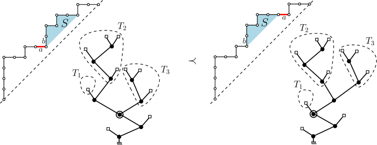
Figure 1. A covering relation in the Tamari lattice, shown on ballot paths and binary trees. The path encodes the postorder of the tree (apart from the first leaf).

Proposition 1.

[4, Prop. 2.1] Let $P$ and $Q$ be two ballot paths of size $n$. Then $Q$ covers $P$ in the Tamari lattice $\mathcal{T}_{n}$ if and only if there exists in $P$ an east step $a$, followed by a north step $b$, such that $Q$ is obtained from $P$ by swapping $a$ and $S$, where $S$ is the shortest factor of $P$ that begins with $b$ and is a (translated) ballot path.

Alternatively, the Tamari lattice $\mathcal{T}_{n}$ is often described in terms of rooted binary trees. The covering relation amounts to a re-organization of three subtrees, often called rotation (Figure 1). The equivalence between the two descriptions is obtained by reading the tree in postorder, and encoding each leaf (resp. inner node) by a north (resp. east) step (apart from the first leaf, which is not encoded). We refer to [4, Sec. 2] for details. The Hasse diagram of the lattice $\mathcal{T}_{n}$ is the 1-skeleton of the associahedron, or Stasheff polytope [11].

A few years ago, Chapoton [12] proved that the number of intervals in $\mathcal{T}_{n}$ (i.e., pairs $P,Q\in\mathcal{T}_{n}$ such that $P\leq Q$) is

$$\frac{2}{n(n+1)}{4n+1\choose n-1}.$$

He observed that this number is known to count 3-connected planar triangulations on $n+3$ vertices [30]. Motivated by this result, Bernardi and Bonichon found a beautiful bijection between Tamari intervals and triangulations [4]. This bijection is in fact a restriction of a more general bijection between intervals in the Stanley lattice and Schnyder woods. A further restriction leads to the enumeration of intervals of the Kreweras lattice.

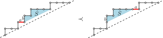
Figure 2. The relation $\prec$ between $m$-ballot paths ($m=2$).

In this paper, we study a generalization of the Tamari lattices to $m$-ballot paths due to Bergeron, and count the intervals of these lattices. Again, a remarkably simple formula holds (see (1)). As we explain below, this formula was first conjectured by F. Bergeron, in connection with the study of coinvariant spaces.

An $m$-ballot path of size $n$ is a path on the square grid consisting of north and east steps, starting at $(0,0)$, ending at $(mn,n)$, and never going below the line $\{x=my\}$. It is a classical exercice to show that there are $\frac{1}{mn+1}{(m+1)n\choose n}$ such paths [14]. Consider the following relation $\prec$ on $m$-ballot paths, illustrated in Figure 2.

Definition 2.

Let $P$ and $Q$ be two $m$-ballot paths of size $n$. Then $P\prec Q$ if there exists in $P$ an east step $a$, followed by a north step $b$, such that $Q$ is obtained from $P$ by swapping $a$ and $S$, where $S$ is the shortest factor of $P$ that begins with $b$ and is a (translated) $m$-ballot path.

As we shall see, the transitive closure of $\prec$ defines a lattice on $m$-ballot paths of size $n$. We call it the $m$-Tamari lattice of size $n$, and denote it by $\mathcal{T}_{n}^{(m)}$. Of course, $\mathcal{T}_{n}^{(1)}$ coincides with $\mathcal{T}_{n}$. See Figure 3 for examples. The main result of this paper is a closed form expression for the number $f_{n}^{(m)}$ of intervals in $\mathcal{T}_{n}^{(m)}$:

$$f_{n}^{(m)}=\frac{m+1}{n(mn+1)}{(m+1)^{2}n+m\choose n-1}.$$ (1)

Figure 3. The $m$-Tamari lattice $\mathcal{T}_{n}^{(m)}$ for $m=1$ and $n=4$ (left) and for $m=2$ and $n=3$ (right). The three walks surrounded by a line in $\mathcal{T}_{4}^{(1)}$ form a lattice that is isomorphic to $\mathcal{T}_{2}^{(2)}$. This will be generalized in Section 2.

The first step of our proof establishes that $\mathcal{T}_{n}^{(m)}$ is in fact isomorphic to a sublattice (and more precisely, an upper ideal) of $\mathcal{T}_{mn}$. We then proceed with a recursive description of the intervals of $\mathcal{T}_{n}^{(m)}$, which translates into a functional equation for the associated generating function (Section 2, Proposition 8). This generating function keeps track of the size of the paths, but also of a catalytic parameter that is needed to write the equation. This parameter is the number of contacts of the lower path with the line $\{x=my\}$. A general theorem asserts that the solution of the equation is algebraic [7], and gives a systematic procedure to solve it for small values of $m$. However, for a generic value of $m$, we have to resort to a guess-and-check approach to solve the equation (Section 3, Theorem 10). We enrich our enumeration by taking into account the initial rise of the upper path, that is, the length of its initial run of north steps. We obtain an unexpected symmetry result: the joint distribution of the number of contacts of the lower path (minus one) and the initial rise of the upper path is symmetric. Section 4 presents comments and questions.

To conclude this introduction, we describe the algebraic problem that led Bergeron to conjecture (1).

Let $X=(x_{i,j})_{{}^{1\leq i\leq\ell}_{1\leq j\leq n}}$ be a matrix of variables, for some positive integers $\ell,n\geq 1$. We call each line of $X$ a set of variables. Let $\mathbb{C}[X]$ be the ring of polynomials in the variables of $X$. The symmetric group ${\mathfrak{S}}_{n}$ acts as a representation on $\mathbb{C}[X]$ by permuting the columns of $X$. That is, if $\sigma\in{\mathfrak{S}}_{n}$ and $f(X)\in\mathbb{C}[X]$, then

$$\sigma(f(X))=f(\sigma(X))=f((x_{i,\sigma(j)})_{{}^{1\leq i\leq\ell}_{1\leq j\leq n}}).$$

We consider the ideal $I$ of ${\mathbb{C}}[X]$ generated by ${\mathfrak{S}}_{n}$-invariant polynomials having no constant term. The quotient ring ${\mathbb{C}}[X]/I$ is (multi-)graded because $I$ is (multi-)homogeneous, and is a representation of ${\mathfrak{S}}_{n}$ because $I$ is invariant under the action of ${\mathfrak{S}}_{n}$. We focus on the dimension of this quotient ring, and to the dimension of the sign subrepresentation. We denote by $W^{\varepsilon}$ the sign subrepresentation of a representation $W$.

Let us begin with the classical case of a single set of variables. When $X=[x_{1},\ldots,x_{n}]$, we consider the coinvariant space $R_{n}$, defined by

$$R_{n}=\mathbb{C}[X]\Big{/}\big{\langle}\big{\{}\sum_{i=1}^{n}x_{i}^{r}\big{|}r\geq 1\big{\}}\big{\rangle},$$

where $\big{\langle}S\big{\rangle}$ denotes the ideal generated by the set $S$. It is known [1] that $R_{n}$ is isomorphic to the regular representation of ${\mathfrak{S}}_{n}$. In particular, $\dim(R_{n})=n!$ and $\dim(R_{n}^{\varepsilon})=1$. There exist explicit bases of $R_{n}$ indexed by permutations.

Let us now move to two sets of variables. In the early nineties, Garsia and Haiman introduced an analogue of $R_{n}$ for $X=\begin{bmatrix}x_{1}&\ldots&x_{n}\\ y_{1}&\ldots&y_{n}\end{bmatrix}$, and called it the diagonal coinvariant space [19]:

$$\operatorname{DR}_{2,n}=\mathbb{C}[X]\Big{/}\big{\langle}\big{\{}\sum_{i=1}^{n}x_{i}^{r}y_{i}^{t}\big{|}r+t\geq 1\big{\}}\big{\rangle}.$$

About ten years later, using advanced algebraic geometry [18], Haiman settled several conjectures of [19] concerning this space, proving in particular that

$$\dim({\operatorname{DR}_{2,n}})=(n+1)^{n-1}\quad\hbox{ and }\quad\dim(\operatorname{DR}_{2,n}^{\ \varepsilon})=\frac{1}{n+1}\binom{2n}{n}.$$ (2)

He also studied an extension of $\operatorname{DR}_{2,n}$ involving an integer parameter $m$ and the ideal $\mathcal{A}$ generated by alternants [16, 17]:

$$\mathcal{A}=\big{\langle}\big{\{}f(x)\big{|}\sigma(f(X))=(-1)^{\operatorname{inv}(\sigma)}f(X),\forall\sigma\in{\mathfrak{S}}_{n}\big{\}}\big{\rangle}.$$

There is a natural action of ${\mathfrak{S}}_{n}$ on the quotient space $\mathcal{A}^{m-1}\big{/}\mathcal{J}\mathcal{A}^{m-1}$. Let us twist this action by the $(m-1)^{\rm st}$ power of the sign representation $\varepsilon$: this gives rise to spaces

$$\mathcal{DR}_{2,n}^{m}:={\varepsilon}^{m-1}\otimes\mathcal{A}^{m-1}\big{/}\mathcal{J}\mathcal{A}^{m-1},$$

so that $\mathcal{DR}_{2,n}^{1}=\mathcal{DR}_{2,n}$. Haiman [18, 17] generalized (2) by proving

$$\dim({\operatorname{DR}_{2,n}^{m}})=(mn+1)^{n-1}\quad\hbox{and }\quad\dim(\operatorname{DR}_{2,n}^{m\ \varepsilon})=\frac{1}{mn+1}\binom{(m+1)n}{n}.$$

Both dimensions have simple combinatorial interpretations: we recognize in the latter the number of $m$-ballot paths of size $n$, and the former is the number of $m$-parking functions of size $n$ (these functions can be described as $m$-ballot paths of size $n$ in which the north steps are labelled from $1$ to $n$ in such a way the labels increase along each run of north steps; see e.g. [31]). However, it is still an open problem to find bases of ${\operatorname{DR}_{2,n}^{m}}$ or $\operatorname{DR}_{2,n}^{m\ \varepsilon}$ indexed by these simple combinatorial objects.

For $\ell\geq 3$, the spaces $\operatorname{DR}_{\ell,n}$ and their generalization ${\operatorname{DR}_{\ell,n}^{m}}$ can be defined similarly. Haiman explored the dimension of $\operatorname{DR}_{\ell,n}$ and $\operatorname{DR}_{\ell,n}^{\ \varepsilon}$. For $\ell=3$, he observed in [19] that, for small values of $n$,

$$\dim({\operatorname{DR}_{3,n}})=2^{n}(n+1)^{n-2}\quad\hbox{and }\quad\dim(\operatorname{DR}_{3,n}^{\ \varepsilon})=\frac{2}{n(n+1)}{4n+1\choose n-1}.$$

Following discussions with Haiman, Bergeron came up with conjectures that directly imply the following generalization (since $\operatorname{DR}_{3,n}^{1}$ coincides with $\operatorname{DR}_{3,n}$):

$$\dim({\operatorname{DR}_{3,n}^{m}})=(m+1)^{n}(mn+1)^{n-2}\quad\hbox{and }\quad\dim(\operatorname{DR}_{3,n}^{m\ \varepsilon})=\frac{m+1}{n(mn+1)}\binom{(m+1)^{2}n+m}{n-1}.$$

Both conjectures are still wide open.

A much simpler problem consists in asking whether these dimensions again have a simple combinatorial interpretation. Bergeron, starting from the sequence $\frac{2}{n(n+1)}{4n+1\choose n-1}$, found in Sloane’s Encyclopedia that this number counts, among others, certain ballot related objects, namely intervals in the Tamari lattice [12]. From this observation, and the role played by $m$-ballot paths for two sets of variables, he was led to introduce the $m$-Tamari lattice $\mathcal{T}_{n}^{(m)}$, and conjectured that $\frac{m+1}{n(mn+1)}\binom{(m+1)^{2}n+m}{n-1}$ is the number of intervals in this lattice. This is the conjecture we prove in this paper. Another of his conjectures is that $(m+1)^{n}(mn+1)^{n-2}$ is the number of Tamari intervals where the larger path is “decorated” by an $m$-parking function [3]. This is proved in [6, 5].

2. A functional equation for the generating function of intervals

The aim of this section is to describe a recursive decomposition of $m$-Tamari intervals, and to translate it into a functional equation satisfied by the associated generating function (Proposition 8). There are two main tools:

• we prove that $\mathcal{T}_{n}^{(m)}$ can be seen as an upper ideal of the usual Tamari lattice $\mathcal{T}_{mn}$,

• we give a simple criterion to decide when two paths of the Tamari lattice are comparable.

2.1. An alternative description of the $m$-Tamari lattices

Our first transformation is totally harmless: we apply a 45 degree rotation to 1-ballot paths to transform them into Dyck paths. A Dyck path of size $n$ consists of steps $(1,1)$ (up steps) and steps $(1,-1)$ (down steps), starts at $(0,0)$, ends at $(0,2n)$ and never goes below the $x$-axis.

We now introduce some terminology, and use it to rephrase the description of the (usual) Tamari lattice $\mathcal{T}_{n}$. Given a Dyck path $P$, and an up step $u$ of $P$, the shortest portion of $P$ that starts with $u$ and forms a (translated) Dyck path is called the excursion of $u$ in $P$. We say that $u$ and the final step of its excursion match each other. Finally, we say that $u$ has rank $i$ if it is the $i^{\hbox{\small th}}$ up step of $P$.

Given two Dyck paths $P$ and $Q$ of size $n$, $Q$ covers $P$ in the Tamari lattice $\mathcal{T}_{n}$ if and only if there exists in $P$ a down step $d$, followed by an up step $u$, such that $Q$ is obtained from $P$ by swapping $d$ and $S$, where $S$ is the excursion of $u$ in $P$. This description implies the following property [4, Cor. 2.2].

Property 3.

If $P\leq Q$ in $\mathcal{T}_{n}$ then $P$ is below $Q$. That is, for $i\in[0..2n]$, the ordinate of the vertex of $P$ lying at abscissa $i$ is at most the ordinate of the vertex of $Q$ lying at abscissa $i$.

Consider now an $m$-ballot path of size $n$, and replace each north step by a sequence of $m$ north steps. This gives a 1-ballot path of size $mn$, and thus, after a rotation, a Dyck path. In this path, for each $i\in[0..n-1]$, the up steps of ranks $mi+1,\ldots,m(i+1)$ are consecutive. We call the Dyck paths satisfying this property $m$-Dyck paths. Clearly, $m$-Dyck paths of size $mn$ are in one-to-one correspondence with $m$-ballot paths of size $n$. Consider now the relation $\prec$ of Definition 2: once reformulated in terms of Dyck paths, it becomes a covering relation in the (usual) Tamari lattice (Figure 4). Conversely, it is easy to check that, if $P$ is an $m$-Dyck path and $Q$ covers $P$ in the usual Tamari lattice, then $Q$ is also an $m$-Dyck path, and the $m$-ballot paths corresponding to $P$ and $Q$ are related by $\prec$. We have thus proved the following result.

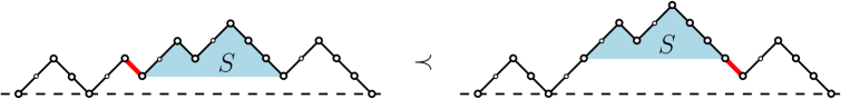
Figure 4. The relation $\prec$ of Figure 2 reformulated in terms of $m$-Dyck paths ($m=2$).

Proposition 4.

The transitive closure of the relation $\prec$ defined in Definition 2 is a lattice on $m$-ballot paths of size $n$. This lattice is isomorphic to the sublattice of the Tamari lattice $\mathcal{T}_{mn}$ consisting of the elements that are larger than or equal to the Dyck path $u^{m}d^{m}\ldots u^{m}d^{m}$. The relation $\prec$ is the covering relation of this lattice.

Notation. From now on, we only consider Dyck paths. We denote by $\mathcal{T}$ the set of Dyck paths, and by $\mathcal{T}_{n}$ the Tamari lattice of Dyck paths of length $n$. By $\mathcal{T}^{(m)}$ we mean the set of $m$-Dyck paths, and by $\mathcal{T}_{n}^{(m)}$ the Tamari lattice of $m$-Dyck paths of size $mn$. This lattice is a sublattice of $\mathcal{T}_{mn}$. Note that $\mathcal{T}^{(1)}=\mathcal{T}$ and $\mathcal{T}_{n}^{(1)}=\mathcal{T}_{n}$.

2.2. Distance functions

Let $P$ be a Dyck path of size $n$. For an up step $u$ of $P$, we denote by $\ell_{P}(u)$ the size of the excursion of $u$ in $P$. The function $D_{P}:[1..n]\to[1..n]$ defined by $D_{P}(i)=\ell(u_{i})$, where $u_{i}$ is the $i^{\hbox{\small{th}}}$ up step of $P$, is called the distance function of $P$. It will sometimes be convenient to see $D_{P}$ as a vector $(\ell(u_{1}),\ldots,\ell(u_{n}))$ with $n$ components. In particular, we will compare distance functions component-wise. The main result of this subsection is a description of the Tamari order in terms of distance functions. This simple characterization seems to be new.

Proposition 5.

Let $P$ and $Q$ be two paths in the Tamari lattice $\mathcal{T}_{n}$. Then $P\leq Q$ if and only if $D_{P}\leq D_{Q}$.

In order to prove this, we first describe the relation between the distance functions of two paths related by a covering relation.

Lemma 6.

Let $P$ be a Dyck path, and $d$ a down step of $P$ followed by an up step $u$. Let $S$ be the excursion of $u$ in $P$, and let $Q$ be the path obtained from $P$ by swapping $d$ and $S$. Let $u^{\prime}$ be the up step matched with $d$ in $P$, and $i_{0}$ the rank of $u^{\prime}$ in $P$. Then $D_{Q}(i)=D_{P}(i)$ for each $i\neq i_{0}$ and $D_{Q}(i_{0})=D_{P}(i_{0})+\ell_{P}(u)$.

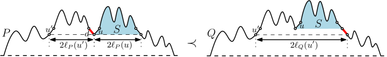
Figure 5. How the distance function changes in a covering relation.

This lemma is easily proved using Figure 5. It already implies that $D_{P}\leq D_{Q}$ if $P\leq Q$. The next lemma establishes the reverse implication, thus concluding the proof of Proposition 5.

Lemma 7.

Let $P$ and $Q$ be two Dyck paths of size $n$ such that $D_{P}\leq D_{Q}$. Then $P\leq Q$ in the Tamari lattice $\mathcal{T}_{n}$.

Proof.

Let us first prove, by induction on the size, that $P$ is below $Q$ (in the sense of Property 3). This is clearly true if $n=0$, so we assume $n>0$.

Let $u$ be the first up step (in $P$ and $Q$). Note that $\ell_{P}(u)=D_{P}(1)\leq D_{Q}(1)=\ell_{Q}(u)$. Let $P^{\prime}$ (resp. $Q^{\prime}$) be the path obtained from $P$ (resp. $Q$) by contracting $u$ and the down step matched with $u$. Observe that $D_{P^{\prime}}$ is obtained by deleting the first component of $D_{P}$, and similarly for $D_{Q^{\prime}}$ and $D_{Q}$. Consequently $D_{P^{\prime}}\leq D_{Q^{\prime}}$, and hence by the induction hypothesis, $P^{\prime}$ is below $Q^{\prime}$. Let us consider momentarily Dyck paths as functions, and write $P(i)=j$ if the vertex of $P$ lying at abscissa $i$ has ordinate $j$. Note that $P(i)=P^{\prime}(i-1)+1$ for $1\leq i<2\ell_{P}(u)$, and $P(i)=P^{\prime}(i-2)$ for $2\ell_{P}(u)\leq i\leq 2n$. Similarly $Q(i)=Q^{\prime}(i-1)+1$ for $1\leq i<2\ell_{Q}(u)$, and $Q(i)=Q^{\prime}(i-2)$ for $2\ell_{Q}(u)\leq i\leq 2n$. Since $\ell_{P}(u)\leq\ell_{Q}(u)$ and $P^{\prime}(i)\leq Q^{\prime}(i)$ for $0\leq i\leq 2n-2$, one easily checks that $P(i)\leq Q(i)$ for $0\leq i\leq 2n$, so that $P$ is below $Q$.

In order to prove that $P\leq Q$, we proceed by induction on $||D_{P}-D_{Q}||$, where $||(x_{1},\ldots,x_{n})||=|x_{1}|+\cdots+|x_{n}|$. If $D_{P}=D_{Q}$ then $P=Q$, because $P$ is below $Q$ and $Q$ is below $P$. So let us assume that $D_{P}\not=D_{Q}$. Let $i$ be minimal such that $D_{P}(i)<D_{Q}(i)$. We claim that $P$ and $Q$ coincide at least until their up step of rank $i$. Indeed, since $P$ lies below $Q$, the paths $P$ and $Q$ coincide up to some abscissa, and then we find a down step $\delta$ in $P$ but an up step in $Q$. Let $j$ be the rank of the up step that matches $\delta$ in $P$. This up step belongs also to $Q$, and, since $\delta\not\in Q$, we have $D_{P}(j)<D_{Q}(j)$. Hence $j\geq i$ by minimality of $i$, and $P$ and $Q$ coincide at least until their up step of rank $i$, which we denote by $u$. Let $d$ be the down step matched with $u$ in $P$ (Figure 6). Since $D_{P}(i)<D_{Q}(i)$, the step $d$ is not a step of $Q$. The step of $Q$ located at the same abscissa as $d$ ends strictly higher than $d$, and in particular, at a positive ordinate. Hence $d$ is not the final step of $P$. Let $s$ be the step following $d$ in $P$.

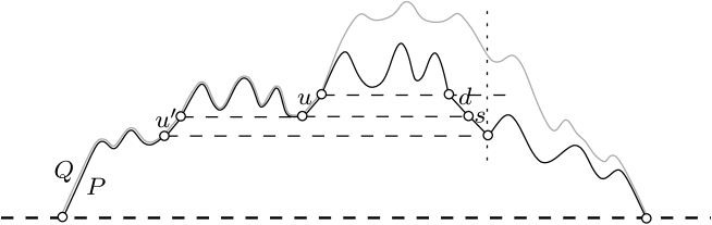
Figure 6. Why $s$ cannot be descending.

Let us prove ad absurdum that $s$ is an up step. Assume $s$ is down. Then $s$ is matched in $P$ with an up step $u^{\prime}$ of rank $j<i$ (Figure 6). Hence $u^{\prime}$ belongs to $Q$ and has rank $j$ in $Q$. Since $s$ cannot belong to $Q$, this implies that $D_{P}(j)<D_{Q}(j)$, which contradicts the minimality of $i$.

Hence $s$ is an up step of $P$ (Figure 7). Let $S$ be the excursion of $s$ in $P$. Since $\ell_{Q}(u)>\ell_{P}(u)$ and since $Q$ is above $P$, we have $\ell_{Q}(u)\geq\ell_{P}(u)+\ell_{P}(s)$, i.e., $D_{Q}(i)\geq D_{P}(i)+\ell_{P}(s)$. Let $P^{\prime}$ be the path obtained from $P$ by swapping $d$ and $S$. Then $P^{\prime}$ covers $P$ in the Tamari lattice. By Lemma 6, $D_{P}=D_{P^{\prime}}$ except at index $i$ (the rank of $u$), where $D_{P^{\prime}}(i)=D_{P}(i)+\ell_{P}(s)$. Since $D_{P}(i)+\ell_{P}(s)\leq D_{Q}(i)$, we have $D_{P^{\prime}}\leq D_{Q}$. But $||D_{P^{\prime}}-D_{Q}||=||D_{P}-D_{Q}||-\ell_{P}(s)$ and by the induction hypothesis, $P^{\prime}\leq Q$ in the Tamari lattice. Hence $P<P^{\prime}\leq Q$, and the lemma is proved.  

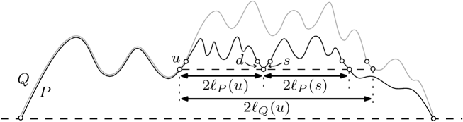
Figure 7. General form of $P$ and $Q$.

2.3. Recursive decomposition of intervals and functional equation

A contact of a Dyck path $P$ is a vertex of $P$ lying on the $x$-axis. It is initial if it is $(0,0)$. A contact of a Tamari interval $[P,Q]$ is a contact of the lower path $P$. The recursive decomposition of intervals that we use makes the number of contacts crucial, and we say that this parameter is catalytic. We also consider another, non-catalytic parameter, which we find to be equidistributed with non-initial contacts (even more, the joint distribution of these two parameters is symmetric). Given an $m$-Dyck path $Q$, the length of the initial run of up steps is of the form $mk$; the integer $k$ is called the initial rise of $Q$. The initial rise of an interval $[P,Q]$ is the initial rise of the upper path $Q$. The aim of this subsection is to establish the following functional equation.

Proposition 8.

For $m\geq 1$, let $F(x)\equiv F^{(m)}(t;x)$ be the generating function of $m$-Tamari intervals, where $t$ counts the size (divided by $m$) and $x$ the number of contacts. Then

$$F(x)=x+xt\left(F(x)\cdot\Delta\right)^{(m)}(F(x)),$$

where $\Delta$ is the following divided difference operator

$$\Delta S(x)=\frac{S(x)-S(1)}{x-1},$$

and the power $m$ means that the operator $G(x)\mapsto F(x)\cdot\Delta G(x)$ is applied $m$ times to $F(x)$.

More generally, if $F(x,y)\equiv F^{(m)}(t;x,y)$ keeps track in addition of the initial rise (via the variable $y$), we have the following functional equation:

$$F(x,y)=x+xyt\left(F(x,1)\cdot\Delta\right)^{(m)}(F(x,y)).$$ (3)

Note that each of the above two equations defines a unique formal power series in $t$ (think of extracting inductively the coefficient of $t^{n}$ in $F^{(m)}(t;x)$ or $F^{(m)}(t;x,y)$).
Examples
1. When $m=1$, the above equation reads

$$F(x,y) = x+xytF(x,1)\cdot\Delta(F(x,y))$$

$$= x+xytF(x,1)\ \frac{F(x,y)-F(1,y)}{x-1}.$$

When $y=1$, we obtain, in the terminology of [7], a quadratic equation with one catalytic variable:

$$F(x)=x+xtF(x)\ \frac{F(x)-F(1)}{x-1}.$$

2. When $m=2$,

$$F(x,y) = x+xyt\ F(x,1)\cdot\Delta(F(x,1)\cdot\Delta(F(x,y)))$$

$$= x+xyt\ F(x,1)\cdot\Delta\left(F(x,1)\ \frac{F(x,y)-F(1,y)}{x-1}\right)$$

$$= x+\frac{xyt}{x-1}\ F(x,1)\ \left(F(x,1)\ \frac{F(x,y)-F(1,y)}{x-1}-F(1,1)F^{\prime}(1,y)\right),$$

where the derivative is taken with respect to the variable $x$. When $y=1$, we obtain a cubic equation with one catalytic variable:

$$F(x)=x+\frac{xt}{x-1}F(x)\ \left(F(x)\ \frac{F(x)-F(1)}{x-1}-F(1)F^{\prime}(1)\right).$$

The solution of (3) will be the topic of the next section. For the moment we focus on the proof of this equation.

We say that a vertex $q$ lies to the right of a vertex $p$ if the abscissa of $q$ is greater than or equal to the abscissa of $p$. A $k$-pointed Dyck path is a tuple $(P;p_{1},\ldots,p_{k})$ where $P$ is a Dyck path and $p_{1},\ldots,p_{k}$ are contacts of $P$ such that $p_{i+1}$ lies to the right of $p_{i}$, for $1\leq i<k$ (note that some $p_{i}$’s may coincide). Given an $m$-Dyck path $P$ of positive size, let $u_{1},\ldots,u_{m}$ be the initial (consecutive) up steps of $P$, and let $d_{1},\ldots,d_{m}$ be the down steps matched with $u_{1},\ldots,u_{m}$, respectively. The $m$-reduction of $P$ is the $m$-pointed Dyck path $(P^{\prime};p_{1},\ldots,p_{m})$ where $P^{\prime}$ is obtained from $P$ by contracting all the steps $u_{1},\ldots,u_{m},d_{1},\ldots,d_{m}$, and $p_{1},\ldots,p_{m}$ are the vertices of $P^{\prime}$ resulting from the contraction of $d_{1},\ldots,d_{m}$. It is easy to check that they are indeed contacts of $P^{\prime}$ (Figure 8).

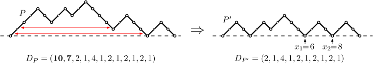
Figure 8. The $m$-reduction of an $m$-Dyck path ($m=2$).

The map $P\mapsto(P^{\prime};p_{1},\ldots,p_{m})$ is clearly invertible, hence $m$-Dyck paths of size $mn$ are in bijection with $m$-pointed $m$-Dyck paths of size $m(n-1)$. Note that the non-initial contacts of $P$ correspond to the contacts of $P^{\prime}$ that lie to the right of $p_{m}$. Note also that the distance function $D_{P^{\prime}}$ (seen as a vector with $m(n-1)$ components) is obtained by deleting the first $m$ components of $D_{P}$. Conversely, denoting by $2x_{i}$ the abscissa of $p_{i}$, $D_{P}$ is obtained by prepending to $D_{P^{\prime}}$ the sequence $(x_{m}+m,x_{m-1}+m-1,\ldots,x_{1}+1)$. In view of Proposition 5, this gives the following recursive characterization of intervals.

Lemma 9.

Let $P$ and $Q$ be two $m$-Dyck paths of size $mn>0$. Let $(P^{\prime};p_{1},\ldots,p_{m})$ and $(Q^{\prime};q_{1},\ldots,q_{m})$ be the $m$-reductions of $P$ and $Q$ respectively. Then $P\leq Q$ in $\mathcal{T}_{n}^{(m)}$ if and only if $P^{\prime}\leq Q^{\prime}$ in $\mathcal{T}_{n-1}^{(m)}$ and for $i\in[1..m]$, the point $q_{i}$ lies to the right of $p_{i}$.

The non-initial contacts of $P$ correspond to the contacts of $P^{\prime}$ located to the right of $p_{m}$.

Let us call $k$-pointed interval in $\mathcal{T}^{(m)}$ a pair consisting of two $k$-pointed $m$-Dyck paths $(P;p_{1},\ldots,p_{k})$ and $(Q;q_{1},\ldots,q_{k})$ such that $P\leq Q$ and for $i\in[1..k]$, the point $q_{i}$ lies to the right of $p_{i}$. An active contact of such a pair is a contact of $P$ lying to the right of $p_{k}$ (if $k=0$, all contacts are declared active). For $0\leq k\leq m$, let us denote by $G^{(m,k)}(t;x,y)\equiv G^{(k)}(x,y)$ the generating function of $k$-pointed $m$-Tamari intervals, where $t$ counts the size (divided by $m$), $x$ the number of active contacts, and $y$ the initial rise (we drop the superscript $m$ since it will not vary). In particular, the series we are interested in is

$$F(x,y)=G^{(0)}(x,y).$$ (4)

Moreover, Lemma 9 implies

$$F(x,y)=x+xyt\ \!G^{(m)}(x,y).$$ (5)

We will prove that, for $k\geq 0$,

$$G^{(k+1)}(x,y)=F(x,1)\cdot\Delta G^{(k)}(x,y).$$ (6)

The functional equation (3) then follows using (4) and (5).

For $k\geq 0$, let $I=[P^{\bullet},Q^{\bullet}]$ be a $(k+1)$-pointed interval in $\mathcal{T}^{(m)}$, with $P^{\bullet}=(P;p_{1},\ldots,p_{k+1})$ and $Q^{\bullet}=(Q;q_{1},\ldots,q_{k+1})$ (see an illustration in Figure 9 when $k=0$). Since $P$ is below $Q$, the contact $q_{k+1}$ of $Q$ is also a contact of $P$. By definition of pointed intervals, $q_{k+1}$ is to the right of $p_{1},\ldots,p_{k+1}$. Decompose $P$ as $P_{\ell}P_{r}$ where $P_{\ell}$ is the part of $P$ to the left of $q_{k+1}$ and $P_{r}$ is the part of $P$ to the right of $q_{k+1}$. Decompose similarly $Q$ as $Q_{\ell}Q_{r}$, where the two factors meet at $q_{k+1}$. The distance function $D_{P}$ (seen as a vector) is $D_{P_{\ell}}$ concatenated with $D_{P_{r}}$, and similarly for $D_{Q}$. In particular, $D_{P_{\ell}}\leq D_{Q_{\ell}}$ and $D_{P_{r}}\leq D_{Q_{r}}$. By Proposition 5, $I_{r}:=[P_{r},Q_{r}]$ is an interval, while $I_{\ell}:=[P^{\circ},Q^{\circ}]$, with $P^{\circ}=(P_{\ell};p_{1},\ldots,p_{k})$ and $Q^{\circ}=(Q_{\ell};q_{1},\ldots,q_{k})$, is a $k$-pointed interval. Its initial rise equals the initial rise of $I$. We denote by $\Phi$ the map that sends $I$ to the pair of intervals $(I_{r},I_{\ell})$.

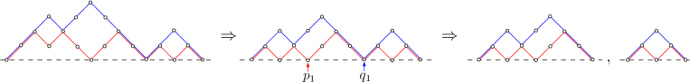
Figure 9. The recursive decomposition of intervals. Starting from an $m$-Tamari interval of size $n$ (here, $m=1$ and $n=7$), one first obtains by reduction an $m$-pointed interval of size $n-1$ (Lemma 9). This interval is further decomposed into two intervals, the first one being $(m-1)$-pointed.

Conversely, take an interval $I_{r}=[P_{r},Q_{r}]$ and a $k$-pointed interval $I_{\ell}=[P^{\circ},Q^{\circ}]$, where $P^{\circ}=(P_{\ell};p_{1},\ldots,p_{k})$ and $Q^{\circ}=(Q_{\ell};q_{1},\ldots,q_{k})$. Let $P=P_{\ell}P_{r}$, $Q=Q_{\ell}Q_{r}$, and denote by $q_{k+1}$ the point where $Q_{\ell}$ and $Q_{r}$ (and $P_{r}$ and $P_{\ell}$) meet. This is a contact of $P$ and $Q$. Then the preimages of $(I_{r},I_{\ell})$ by $\Phi$ are all the intervals $I=[P^{\bullet},Q^{\bullet}]$ such that $P^{\bullet}=(P;p_{1},\ldots,p_{k+1})$ and $Q^{\bullet}=(Q;q_{1},\ldots,q_{k+1})$, where $p_{k+1}$ is any active contact of $P_{\ell}$. If $P_{\ell}$ has $i$ active contacts and $P_{r}$ has $j$ contacts, then $(I_{r},I_{\ell})$ has $i$ preimages, having respectively $j,1+j,\ldots,i+j-1$ active contacts ($j$ active contacts when $p_{k+1}=q_{k+1}$, and $i+j-1$ active contacts when $p_{k+1}=p_{k}$). Let us write $G^{(k)}(x,y)=\sum_{i\geq 0}G^{(k)}_{i}(y)x^{i}$, so that $G^{(k)}_{i}(y)$ counts (by the size and the initial rise) $k$-pointed intervals with $i$ active contacts. The above discussion gives

$$G^{(k+1)}(x,y) = F(x,1)\sum_{i\geq 1}G^{(k)}_{i}(y)(1+x+\cdots+x^{i-1})$$

$$= F(x,1)\sum_{i\geq 1}G^{(k)}_{i}(y)\frac{x^{i}-1}{x-1}$$

$$= F(x,1)\cdot\Delta G^{(k)}(x,y),$$

as claimed in (6). The factor $F(x,1)$ accounts for the choice of $I_{r}$, and the term $\Delta G^{(k)}(x,y)$ for the choice of $I_{\ell}$ and $p_{k+1}$. This completes the proof of Proposition 8.  

3. Solution of the functional equation

In this section, we solve the functional equation of Proposition 8, and thus establish the main result of this paper. We obtain in particular an unexpected symmetry property: the series $yF^{(m)}(t;x,y)$ is symmetric in $x$ and $y$. In other words, the joint distribution of the number of non-initial contacts (of the lower path) and the initial rise (of the upper path) is symmetric.

For any ring $\mathbb{A}$, we denote by $\mathbb{A}[x]$ the ring of polynomials in $x$ with coefficients in $\mathbb{A}$, and by $\mathbb{A}[[x]]$ the ring of formal power series in $x$ with coefficients in $\mathbb{A}$. This notation is extended to the case of polynomials and series in several indeterminates $x_{1},x_{2},\ldots$

Theorem 10.

For $m\geq 1$, let $F^{(m)}(t;x,y)$ be the generating function  of $m$-Tamari intervals, where $t$ counts the size (divided by $m$), $x$ the number of contacts of the bottom path, and $y$ the initial rise of the upper path. Let $z$, $u$ and $v$ be three indeterminates, and set

$$t=z(1-z)^{m^{2}+2m},\quad x=\frac{1+u}{(1+zu)^{m+1}},\quad\hbox{and}\quad y=\frac{1+v}{(1+zv)^{m+1}}.$$ (7)

Then $F^{(m)}(t;x,y)$ becomes a formal power series in $z$ with coefficients in ${\mathbb{Q}}[u,v]$, and this series is rational. More precisely,

$$yF^{(m)}(t;x,y)=\frac{(1+u)(1+zu)(1+v)(1+zv)}{(u-v)(1-zuv)(1-z)^{m+2}}\left(\frac{1+u}{(1+zu)^{m+1}}-\frac{1+v}{(1+zv)^{m+1}}\right).$$ (8)

In particular, $yF^{(m)}(t;x,y)$ is a symmetric series in $x$ and $y$.

Remark. This result was first guessed for small values of $m$. More precisely, we first guessed the values of $\frac{\partial^{i}F}{\partial x}(1,1)$ for $0\leq i\leq m-1$, and then combined these conjectured values with the functional equation to obtain conjectures for $F(x,1)$ and $F(x,y)$. Let us illustrate our guessing procedure on the case $m=1$. We first consider the case $y=1$, where the equation reads

$$F(x,1)=x+xtF(x,1)\frac{F(x,1)-F(1,1)}{x-1}.$$ (9)

Our first objective is to guess the value of $F(1,1)$. Using the above equation, we easily compute, say, the 20 first coefficients of $F(1,1)$. Using the Maple package gfun [27], we conjecture from this list of coefficients that $f\equiv F(1,1)$ satisfies

$$1-16\,t-\left(1-20\,t\right)f-\left(3\,t+8\,{t}^{2}\right){f}^{2}-3\,{t}^{2}{f}^{3}-{t}^{3}{f}^{4}=0.$$

Using the package algcurves, we find that the above equation admits a rational parametrization, for instance

$$t=z(1-z)^{3},\quad f=F(1,1)=\frac{1-2z}{(1-z)^{3}}.$$

This is the end of the “guessing” part. Assume the above identity holds, and replace $t$ and $F(1,1)$ in (9) by their expressions in terms of $z$. This gives an algebraic equation in $F(x,1)$, $x$ and $z$. Again, the package algcurves reveals that this equation, seen as an equation in $F(x,1)$ and $x$, has a rational parametrization, for instance

$$x=\frac{1+u}{(1+zu)^{2}},\quad F(x,1)={\frac{\left(1+u\right)\left(1-2\,z-{z}^{2}u\right)}{\left(1+zu\right)\left(1-z\right)^{3}}}.$$

Let us finally return to the functional equation defining $F(x,y)$:

$$F(x,y)=x+xytF(x,1)\frac{F(x,y)-F(1,y)}{x-1}.$$

In this equation, replace $t$, $x$ and $F(x,1)$ by their conjectured expressions in terms of $z$ and $u$. This gives

$$\left(1+zu-zy\frac{(1+u)^{2}}{u}\right)F(x,y)={\frac{1+u}{1+zu}}-zy\frac{(1+u)^{2}}{u}F(1,y).$$ (10)

We conclude by applying to this equation the kernel method (see, e.g. [2, 8, 26]): let $U\equiv U(z;y)$ be the unique formal power series in $z$ (with coefficients in ${\mathbb{Q}}[y]$) satisfying

$$U=zy{(1+U)^{2}}-zU^{2}.$$

Equivalently,

$$U=z\frac{1+v}{1-2z-z^{2}v},\quad\hbox{with}\quad y=\frac{1+v}{(1+zv)^{2}}.$$

Setting $u=U$ in (10) cancels the left-hand side, and thus the right-hand side, giving

$$yF(1,y)={\frac{\left(1+v\right)\left(1-2\,z-{z}^{2}v\right)}{\left(1+zv\right)\left(1-z\right)^{3}}}.$$

A conjecture for the trivariate series $F(t;x,y)$ follows, using (10). This conjecture coincides with (8). $\hfill{\Box}$

Before we prove Theorem 10, let us give a closed form expression for the number of intervals in $\mathcal{T}_{n}^{(m)}$.

Corollary 11.

Let $m\geq 1$ and $n\geq 1$. The number of intervals in the Tamari lattice $\mathcal{T}_{n}^{(m)}$ is

$$f_{n}^{(m)}=\frac{\bar{m}}{n(mn+1)}{n\bar{m}^{2}+m\choose n-1},$$

where we denote $\bar{m}=m+1$. For $2\leq i\leq n+1$, the number of intervals in which the bottom path has $i$ contacts with the $x$-axis is

$$f_{n,i}^{(m)}=\frac{(n\bar{m}^{2}-i\bar{m}+m)!(i\bar{m}-m)!}{(n\bar{m}^{2}-n-im+2m)!(n-i+1)!(mi)!(i-2)!}P_{m}(n,i),$$ (11)

where $P_{m}(n,i)$ is a polynomial in $n$ and $i$. In particular,

$$P_{1}(n,i)=2,\quad P_{2}(n,i)=6(33\,in-9\,{i}^{2}+15\,i-2\,n-2).$$

More generally,

$$i(i-1)P_{m}(n,i)=-\bar{m}!(m-1)!(n-i+1){{i\bar{m}}\choose m}{{nm(m+2)-im+2m}\choose m-1}\\ +\sum_{k=1}^{m-2}kk!^{2}(m-k-2)!(m-k-1)!((i+1)m\bar{m}+2\bar{m}+k)(n-i)(n-i+1)\times\\ {{i\bar{m}-k-1}\choose m-k-1}{im\choose k}{{n\bar{m}^{2}-i\bar{m}+m+k}\choose k}{{nm(m+2)-im+2m}\choose{m-k-2}}\\ +m!^{2}{im\choose m-1}\left(i{n\bar{m}^{2}-i\bar{m}+2m\choose m}-\frac{(m-1)(i\bar{m}+2)(n-i+1)}{m}{n\bar{m}^{2}-i\bar{m}+2m-1\choose m-1}\right).$$ (12)

Remarks
1. The case $m=1$ of (11) reads

$$f_{n,i}^{(1)}=\frac{(i-1)(4n-2i+1)!}{(3n-i+2)!(n-i+1)!}{2i\choose i}.$$

This result can also obtained using Bernardi and Bonichon’s bijection between intervals of size $n$ in the (usual) Tamari lattice and planar 3-connected triangulations having $n+3$ vertices [4]. Indeed, through this bijection, the number of contacts in the lower path of the interval becomes the degree of the root-vertex of the triangulation, minus one [4, Def. 3.2]. The above result is thus equivalent to a result of Brown counting triangulations by the number of vertices and the degree of the root-vertex [10, Eq. (4.7)].

2. Our expression of $P_{m}$ is not illuminating, but we have given it to prove that $P_{m}$ is indeed a polynomial. If we fix $i$ rather than $m$, then, experimentally, $P_{m}(n,i)$ seems to be a sum of two hypergeometric terms in $m$ and $n$. More precisely, it appears that

$$P_{m}(n,i)=\frac{m\bar{m}!(im)!}{(i\bar{m}-m)!{n\choose{i-1}}}\times\\ \left(\bar{m}R_{i}(m,n){n\bar{m}^{2}-(i-2)\bar{m}-1\choose\bar{m}}+Q_{i}(m,n){nm(m+2)-(i-2)m\choose m}\right),$$

where $R_{i}$ and $Q_{i}$ are two polynomials in $m$ and $n$. This holds at least for small values of $i$.

3. The coefficients of the trivariate series $F(t;x,y)$ do not seem to have small prime factors, even when $m=1$.

Proof of Theorem 10. The functional equation of Proposition 8 defines a unique formal power series in $t$ (think of extracting inductively the coefficient of $t^{n}$ in $F(t;x,y)$). The coefficients of this series are polynomials in $x$ and $y$. The parametrized expression of $F(t;x,y)$ given in Theorem 10 also defines $F(t;x,y)$ uniquely as a power series in $t$, because (7) defines $z$, $u$ and $v$ uniquely as formal power series in $t$ (with coefficients in ${\mathbb{Q}}$, ${\mathbb{Q}}[x]$ and ${\mathbb{Q}}[y]$ respectively). Thus it suffices to prove that the series $F(t;x,y)$ of Theorem 10 satisfies the equation of Proposition 8.

If $G(t;x,y)\equiv G(x,y)$ is any series in ${\mathbb{Q}}[x,y][[t]]$, then performing the change of variables (7) gives $G(t;x,y)=H(z;u,v)$, where

$$H(z;u,v)\equiv H(u,v)=G\left(z(1-z)^{m^{2}+2m};\frac{1+u}{(1+zu)^{m+1}},\frac{1+v}{(1+zv)^{m+1}}\right).$$

Moreover, if $F(x,y)$ is given by (8), then

$$F(x,1)=\frac{(1+u)(1+zu)}{u(1-z)^{m+2}}\left(\frac{1+u}{(1+zu)^{m+1}}-1\right),$$

and

$$F(x,1)\Delta G(x,y)=\frac{(1+u)(1+zu)}{(1-z)^{m+2}}\frac{H(u,v)-H(0,v)}{u}.$$

Let us define an operator $\Lambda$ as follows: for any series $H(z;u,v)\in{\mathbb{Q}}[u,v][[z]]$,

$$\Lambda H(z;u,v):=(1+u)(1+zu)\frac{H(z;u,v)-H(z;0,v)}{u}.$$ (13)

Then the series $F(t;x,y)$ of Theorem 10 satisfies the equation of Proposition 8 if and only if the series $H(u,v)$ obtained by performing the change of variables (7) in $y(1-z)^{m+2}F(x,y)$, that is,

$$H(u,v)=\frac{(1+u)(1+zu)(1+v)(1+zv)}{(u-v)(1-zuv)}\left(\frac{1+u}{(1+zu)^{m+1}}-\frac{1+v}{(1+zv)^{m+1}}\right).$$ (14)

satisfies

$$z\Lambda^{(m)}H(u,v)=\frac{(1+zu)^{m+1}(1+zv)^{m+1}}{(1+u)(1+v)}H(u,v)-(1-z)^{m+2}.$$ (15)

Hence we simply have to prove an identity on rational functions. Observe that both $H(u,v)$ and the conjectured expression of $\Lambda^{(m)}H(u,v)$ are symmetric in $u$ and $v$. More generally, computing (with the help of Maple) the rational functions $\Lambda^{(k)}H(u,v)$ for a few values of $m$ and $k$ suggests that these fractions are always symmetric in $u$ and $v$. This observation raises the following question: Given a symmetric function $H(u,v)$, when is $\Lambda H(u,v)$ also symmetric? This leads to the following lemma, which will reduce the proof of (15) to the case $v=0$.

Lemma 12.

Let $H(z;u,v)\equiv H(u,v)$ be a series of ${\mathbb{Q}}[u,v][[z]]$, symmetric in $u$ and $v$. Let $\Lambda$ be the operator defined by (13), and denote $H_{1}(u,v):=\Lambda H(u,v)$. Then $H_{1}(u,v)$ is symmetric in $u$ and $v$ if and only if $H$ satisfies

$$H(u,v)=\frac{u(1+v)(1+zv)H(u,0)-v(1+u)(1+zu)H(v,0)}{(u-v)(1-zuv)}.$$ (16)

If this holds, then $H_{1}(u,v)$ also satisfies (16) (with $H$ replaced by $H_{1}$). By induction, the same holds for $H_{k}(u,v):=\Lambda^{(k)}H(u,v)$.

The proof is a straightforward calculation. 

Note that a series $H$ satisfying (16) is characterized by the value of $H(u,0)$. The series $H(u,v)$ given by (14) satisfies (16), with

$$H(u,0)=\frac{(1+u)(1+zu)}{u}\left({\frac{1+u}{(1+zu)^{m+1}}-1}\right)=\Lambda\left(\frac{1+u}{(1+zu)^{m+1}}\right).$$

Moreover, one easily checks that the right-hand side of (15) also satisfies (16), as expected from Lemma 12. Thus it suffices to prove the case $v=0$ of (15), namely

$$z\Lambda^{(m+1)}\left(\frac{1+u}{(1+zu)^{m+1}}\right)=\frac{(1+u)(1+zu)}{u}\left(1-\frac{(1+zu)^{m+1}}{1+u}\right)-(1-z)^{m+2}.$$ (17)

This will be a simple consequence of the following lemma.

Lemma 13.

Let $\Lambda$ be the operator defined by (13). For $m\geq 1$,

$$\Lambda^{(m)}\left(\frac{1}{(1+zu)^{m}}\right)=(1-z)^{m}-(1+zu)^{m}.$$

Proof.

We will actually prove a more general identity. Let $1\leq k\leq m$, and denote $w=1+zu$. Then

$$\Lambda^{(k)}\left(\frac{1}{(1+zu)^{m}}\right)=\frac{(1-z)^{k}}{w^{m-k}}-\sum_{i=k}^{m-1}\sum_{j=1}^{k}\frac{(-1)^{k+j}z^{k-j+1}}{w^{m-i-1}}{k\choose j-1}{i-j+1\choose k-j}\\ +\sum_{i=1}^{k-1}\sum_{j=1}^{i}(-1)^{j-1}z^{j}w^{k-i}{i-1\choose j-1}{m-k+j-1\choose j}-w^{k}.$$ (18)

The case $k=m$ is the identity of Lemma 13. In order to prove (18), we need an expression of $\Lambda(w^{p})$, for all $p\in{\mathbb{Z}}$. Using the definition (13) of $\Lambda$, one obtains, for $p\geq 1$,

$$\left\{\begin{array}[]{lll}\displaystyle\Lambda\left(\frac{1}{w^{p}}\right)&=&\displaystyle\frac{1-z}{w^{p-1}}-z\sum_{a=0}^{p-2}\frac{1}{w^{a}}-w,\\ \displaystyle\Lambda(1)&=&0,\\ \displaystyle\Lambda\left({w^{p}}\right)&=&\displaystyle(z-1)w+z\sum_{a=2}^{p}w^{a}+w^{p+1}.\end{array}\right.$$ (19)

We now prove (18), by induction on $k\geq 1$. For $k=1$, (18) coincides with the expression of $\Lambda(1/w^{p})$ given above (with $p$ replaced by $m$). Now let $1\leq k<m$. Apply $\Lambda$ to (18), use (19) to express the terms $\Lambda(w^{p})$ that appear, and then check that the coefficient of $w^{a}z^{b}$ is what it is expected to be, for all values of $a$ and $b$. The details are a bit tedious, but elementary. One needs to apply a few times the following identity:

$$\sum_{r=r_{1}}^{r_{2}}{r-a\choose b}={\frac{\left(r_{2}+1-a-b\right)}{b+1}}{r_{2}+1-a\choose b}-{\frac{\left(r_{1}-a-b\right)}{b+1}}{r_{1}-a\choose b}.$$

We give in the appendix a constructive proof of Lemma 13, which does not require to guess the more general identity (18). It is also possible to derive (18) combinatorially from (19) using one-dimensional lattice paths (in this setting, (19) describes what steps are allowed if one starts at position $p$, for any $p\in{\mathbb{Z}}$).  

Let us now return to the proof of (17). We write

$$z\frac{1+u}{(1+uz)^{m+1}}=\frac{1}{(1+uz)^{m}}+\frac{z-1}{(1+uz)^{m+1}}.$$

Thus

$$z\Lambda^{(m+1)}\left(\frac{1+u}{(1+uz)^{m+1}}\right) = \Lambda\left(\Lambda^{(m)}\left(\frac{1}{(1+uz)^{m}}\right)\right)+(z-1)\Lambda^{(m+1)}\left(\frac{1}{(1+uz)^{m+1}}\right)$$

$$= \Lambda\left((1-z)^{m}-(1+uz)^{m}\right)+(z-1)\left((1-z)^{m+1}-(1+uz)^{m+1}\right)$$

by Lemma 13. Eq. (17) follows, and Theorem 10 is proved.  

Proof of Corollary 11. Let us first determine the coefficients of $F(t;1,1)$. By letting $u$ and $v$ tend to $0$ in the expression of $yF(t;x,y)$, we obtain

$$F(t;1,1)=\frac{1-(m+1)z}{(1-z)^{m+2}},$$

where $t=z(1-z)^{m^{2}+2m}$. The Lagrange inversion formula gives

$$[t^{n}]F(t;1,1)=\frac{1}{n}[t^{n-1}]\frac{1-(m+1)^{2}t}{(1-t)^{nm(m+2)+m+3}},$$

and the expression of $f_{n}^{(m)}$ follows after an elementary coefficient extraction.

We now wish to express the coefficient of $t^{n}x^{i}$ in

$$F(t;x,1)=\frac{(1+u)(1+zu)}{u(1-z)^{m+2}}\left(\frac{1+u}{(1+zu)^{m+1}}-1\right).$$

We will expand this series, first in $x$, then in $t$, applying the Lagrange inversion formula first to $u$, then to $z$. We first expand $(1-z)^{m+2}F(t;x,1)$ in partial fractions of $u$:

$$(1-z)^{m+2}F(t;x,1)=-z\mathbbm{1}_{m>1}-(1+zu)-\sum_{k=1}^{m-2}\frac{z}{(1+uz)^{k}}+\frac{1-z^{2}}{z(1+uz)^{m-1}}-\frac{(1-z)^{2}}{z(1+uz)^{m}}.$$

By the Lagrange inversion formula, applied to $u$, we have, for $i\geq 1$ and $p\geq-m$,

$$[x^{i}](1+zu)^{p}=\frac{p}{i}{{i\bar{m}+p-1}\choose{i-1}}z^{i}(1-z)^{im+p},$$

with $\bar{m}=m+1$. Hence, for $i\geq 1$,

$$i[x^{i}]F(t;x,1)=-{i\bar{m}\choose i-1}z^{i}(1-z)^{(i-1)m-1}+\sum_{k=1}^{m-2}k{{i\bar{m}-k-1}\choose{i-1}}z^{i+1}(1-z)^{(i-1)m-k-2}\\ -(m-1){{i\bar{m}-m}\choose i-1}z^{i-1}(1+z)(1-z)^{(i-2)m}+m{{(i-1)\bar{m}}\choose{i-1}}z^{i-1}(1-z)^{(i-2)m}.$$

We rewrite the above line as

$${{i\bar{m}-m}\choose{i-1}}\left(\frac{i}{i\bar{m}-m}z^{i-1}(1-z)^{(i-2)m}-(m-1)z^{i}(1-z)^{(i-2)m}\right).$$

Recall that $z=\frac{t}{(1-z)^{m^{2}+2m}}$. Hence, for $i\geq 1$,

$$i[x^{i}t^{n}]F(t;x,1)=-{i\bar{m}\choose i-1}[t^{n-i}]\frac{1}{(1-z)^{\bar{m}(im+1)}}\\ +\sum_{k=1}^{m-2}k{{i\bar{m}-k-1}\choose{i-1}}[t^{n-i-1}]\frac{1}{(1-z)^{(i+1)m\bar{m}+2\bar{m}+k}}\\ +{{i\bar{m}-m}\choose i-1}\left(\frac{i}{i\bar{m}-m}[t^{n-i+1}]\frac{1}{(1-z)^{m(i\bar{m}-m)}}-(m-1)[t^{n-i}]\frac{1}{(1-z)^{m(i\bar{m}+2)}}\right).$$

By the Lagrange inversion formula, applied to $z$, we have, for $p\geq 1$ and $n\geq 1$,

$$[t^{n}]\frac{1}{(1-z)^{p}}=\frac{p}{n}{n\bar{m}^{2}+p-1\choose{n-1}}.$$

This formula actually holds for $n=0$ if we write it as

$$[t^{n}]\frac{1}{(1-z)^{p}}=\frac{p\,(n\bar{m}^{2}+p-1)!}{n!\,(n\bar{m}^{2}-n+p)!},$$

and actually for $n<0$ as well with the convention ${a\choose{n-1}}=0$ if $n<0$. With this convention, we have, for $1\leq i\leq n+1$,

$$i[x^{i}t^{n}]F(t;x,1)=-\frac{\bar{m}(im+1)}{n-i}{i\bar{m}\choose i-1}{{n\bar{m}^{2}-i\bar{m}+m}\choose{n-i-1}}\\ +\sum_{k=1}^{m-2}k\frac{(i+1)m\bar{m}+2\bar{m}+k}{n-i-1}{{i\bar{m}-k-1}\choose{i-1}}{{n\bar{m}^{2}-i\bar{m}+m+k}\choose{n-i-2}}\\ +m{{i\bar{m}-m}\choose{i-1}}\left(\frac{i}{n-i+1}{{n\bar{m}^{2}-i\bar{m}+2m}\choose{n-i}}-(m-1)\frac{i\bar{m}+2}{n-i}{{n\bar{m}^{2}-i\bar{m}+2m-1}\choose n-i-1}\right).$$

This gives the expression (11) of $f_{n,i}^{(m)}$, with $P_{m}(n,i)$ given by (12). Clearly, $i(i-1)P_{m}(n,i)$ is a polynomial in $n$ and $i$, but we still have to prove that it is divisible by $i(i-1)$.

For $m\geq 1$ and $1\leq k\leq m-2$, the polynomials ${i\bar{m}\choose m}$ and ${im\choose k}$ are divisible by $i$. The next-to-last term of (12) contains an explicit factor $i$. The last term vanishes if $m=1$, and otherwise contains a factor ${im\choose m-1}$, which is a multiple of $i$. Hence each term of (12) is divisible by $i$.

Finally, the right-hand side of (12) is easily evaluated to be 0 when $i=1$, using the sum function of Maple.  

4. Final comments

Bijective proofs? Given the simplicity of the numbers (1), it is natural to ask about a bijective enumeration of $m$-Tamari intervals. A related question would be to extend the bijection of [4] (which transforms 1-Tamari intervals into triangulations) into a bijection between $m$-Tamari intervals and certain maps (or related structures, like balanced trees or mobiles [28, 9]). Counting these structures in a bijective way (as is done in [25] for triangulations) would then provide a bijective proof of (1).

Symmetry. The fact that the joint distribution of the number of non-initial contacts of the lower path and the initial rise of the upper path is symmetric remains a combinatorial mystery to us, even when $m=1$. What is easy to see is that the joint distribution of the number of non-initial contacts of the lower path and the final descent of the upper path is symmetric. Indeed, there exists a simple involution on Dyck paths that reverses the Tamari order and exchanges these two parameters: If we consider Dyck paths as postorder encodings of binary trees, this involution amounts to a simple reflection of trees. Via the bijection of [4], these two parameters correspond to the degrees of two vertices of the root-face of the triangulation [4, Def. 3.2], so that the symmetry is also clear in this setting.

A $q$-analogue of the functional equation. As described in the introduction, the numbers $f_{n}^{(m)}$ are conjectured to give the dimension of certain polynomial rings $\operatorname{DR}_{3,n}^{m\ \varepsilon}$. These rings are tri-graded (with respect to the sets of variables $\{x_{i}\}$, $\{y_{i}\}$ and $\{z_{i}\}$), and it is conjectured [3] that the dimension of the homogeneous component in the $x_{i}$’s of degree $k$ is the number of intervals $[P,Q]$ in $\mathcal{T}_{n}^{(m)}$ such that the longest chain from $P$ to $Q$, in the Tamari order, has length $k$. One can recycle the recursive description of intervals described in Section 2.3 to generalize the functional equation of Proposition 8, taking into account (with a new variable $q$) this distance. Eq. (3) remains valid, upon defining the operator $\Delta$ by

$$\Delta S(x)=\frac{S(qx)-S(1)}{qx-1}.$$

The coefficient of $t^{n}$ in the series $F(t,q;x,y)$ does not seem to factor, even when $x=y=1$. The coefficients of the bivariate series $F(t,q;1,1)$ have large prime factors.

More on $m$-Tamari lattices? We do not know of any simple description of the $m$-Tamari lattice in terms of rotations in $m+1$-ary trees (which are equinumerous with $m$-Dyck paths). A rotation for ternary trees is defined in [23], but does not give a lattice. However, as noted by the referee, if we interpret $m$-ballot paths as the prefix (rather than postfix) code of an $m+1$-ary tree, the covering relation can be described quite simply. One first chooses a leaf $\ell$ that is followed (in prefix order) by an internal node $v$. Then, denoting by $T_{0},\ldots,T_{m}$ the $m+1$ subtrees attached to $v$, from left to right, we insert $v$ and its first $m$ subtrees in place of the leaf $\ell$, which becomes the rightmost child of $v$. The rightmost subtree of $v$, $T_{m}$, finally takes the former place of $v$ (Figure 10).

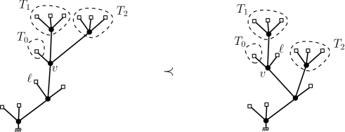
Figure 10. The covering relation of Figure 2 translated in terms of ternary trees.

More generally, it may be worth exploring analogues for the $m$-Tamari lattices of the numerous questions that have been studied for the usual Tamari lattice. To mention only one, what is the diameter of the $m$-Tamari lattice, that is, the maximal distance between two $m$-Dyck paths in the Hasse diagram? When $m=1$, it is known to be $2n-6$ for $n$ large enough, but the proof is as complicated as the formula is simple [13, 29].

$$\triangleleft\;\lhd\;\diamond\;\rhd\;\triangleright$$

Acknowledgements. We are grateful to François Bergeron for advertising in his lectures the conjectural interpretation of the numbers (1) in terms of Tamari intervals. We also thank Gwendal Collet and Gilles Schaeffer for interesting discussions on this topic.

$$\triangleleft\;\lhd\;\diamond\;\rhd\;\triangleright$$

Appendix. A constructive approach to Lemma 13. In order to prove Lemma 13, we had to prove the more general identity (18). This identity was first guessed by expanding $\Lambda^{(k)}(1/w^{m})$ in $w$ and $z$, for several values of $k$ and $m$. Fortunately, the coefficients in this expansion turned out to be simple products of binomial coefficients.

What if these coefficients had not been so simple? A constructive approach goes as follows. Introduce the following two formal power series in $t$ and $s$, with coefficients in ${\mathbb{Q}}[w,1/w,z]$:

$$P(t;s)=\sum_{m\geq 1,k\geq 0}t^{k}s^{m-1}\Lambda^{(k)}(w^{m})\quad\hbox{and}\quad N(t;s)=\sum_{m\geq 0,k\geq 0}t^{k}s^{m}\Lambda^{(k)}\left(\frac{1}{w^{m}}\right),$$

where we still denote $w=1+zu$. Observe that

$$P(t;0)=\sum_{k\geq 0}t^{k}\Lambda^{(k)}(w).$$

We want to compute the coefficient of $t^{m}s^{m}$ of $N(t;s)$, since this coefficient is $\Lambda^{(m)}(1/w^{m})$.

Eq. (19) yield functional equations for the series $P$ and $N$. For $P(t;s)$ first,

$$P(t;s) = \sum_{m\geq 1}s^{m-1}w^{m}+t\sum_{m\geq 1,k\geq 1}t^{k-1}s^{m-1}\Lambda^{(k-1)}\left((z-1)w+z\sum_{a=2}^{m}w^{a}+w^{m+1}\right)$$

$$= \frac{w}{1-sw}+\frac{t(z-1)}{1-s}P(t;0)+\frac{tz}{1-s}\left(P(t;s)-P(t;0)\right)+t\,\frac{P(t;s)-P(t;0)}{s}.$$

Equivalently,

$$\left(1-\frac{tz}{1-s}-\frac{t}{s}\right)P(t;s)=\frac{w}{1-sw}-\frac{tP(t;0)}{s(1-s)}.$$ (20)

Now for $N(t;s)$, we have

$$N(t;s) = \sum_{m\geq 0}\frac{s^{m}}{w^{m}}+t\sum_{m\geq 1,k\geq 1}t^{k-1}s^{m}\Lambda^{(k-1)}\left(\frac{1-z}{w^{m-1}}-z\sum_{a=0}^{m-2}\frac{1}{w^{a}}-w\right)$$

$$= \frac{1}{1-s/w}+ts(1-z)N(t;s)-\frac{tzs^{2}}{1-s}N(t;s)-\frac{ts}{1-s}P(t;0).$$

Equivalently,

$$\left(1-ts+\frac{tzs}{1-s}\right)N(t;s)=\frac{1}{1-s/w}-\frac{ts}{1-s}P(t;0).$$ (21)

Equation (20) can be solved using the kernel method (see e.g. [2, 8, 26]): let $S\equiv S(t,z)$ be the unique formal power series in $t$, with coefficients in ${\mathbb{Q}}[z]$, having constant term 0 and satisfying

$$1-\frac{tz}{1-S}-\frac{t}{S}=0.$$

That is,

$$S=\frac{1+t-tz-\sqrt{1-2t(1+z)+t^{2}(1-z)^{2}}}{2}.$$ (22)

Then setting $s=S$ cancels the left-hand side of (20), giving

$$P(t;0)=\frac{wS(1-S)}{t(1-wS)}.$$

Combined with (21), this yields an explicit expression of $N(t;s)$:

$$N(t;s)=\frac{1}{1-ts+\frac{tzs}{1-s}}\left(\frac{1}{1-s/w}-\frac{wsS(1-S)}{(1-s)(1-wS)}\right).$$

We want to extract from this series the coefficient of $t^{m}s^{m}$, and obtain the simple expression $(1-z)^{m}-w^{m}$ predicted by Lemma 13. Clearly, the first part of the above expression of $N(t;s)$ (with non-positive powers of $w$) contributes $(1-z)^{m}$, as expected. For $i\geq 1$, the coefficient of $w^{i}$ in the second part of $N(t;s)$ is

$$R_{i}:=-\frac{sS^{i}(1-S)}{(1-s)\left(1-ts+\frac{tzs}{1-s}\right)}.$$

Recall that $S$, given by (22), depends on $t$ and $z$, but not on $s$. Since $S=t+O(t^{2})$, the coefficient of $t^{m}s^{m}$ in $R_{i}$ is zero for $i>m$. When $i=m$, it is easily seen to be $-1$, as expected. In order to prove that the coefficient of $t^{m}s^{m}$ in $R_{i}$ is zero when $0<i<m$, we first perform a partial fraction expansion of $R_{i}$ in $s$, using

$$(1-s)\left(1-ts+\frac{tzs}{1-s}\right)=(1-sS)(1-st/S),$$

where $S$ is defined by (22). This gives

$$R_{i}=-\frac{S^{i+1}(1-S)}{t-S^{2}}\left(\frac{1}{1-ts/S}-\frac{1}{1-sS}\right),$$

so that

$$[s^{m}]R_{i}=-\frac{S^{i+1-m}(1-S)}{t-S^{2}}\left(t^{m}-S^{2m}\right)=\sum_{j=0}^{m-1}t^{m-1-j}S^{2j+i-m+1}(S-1)$$

and

$$[s^{m}t^{m}]R_{i}=\sum_{j=0}^{m-1}[t^{j+1}]S^{2j+i-m+1}(S-1)=\sum_{j=0}^{m-i}[t^{j+1}]S^{2j+i-m+1}(S-1).$$ (23)

The Lagrange inversion gives, for $n\geq 1$ and $k\in{\mathbb{Z}}$,

$$[t^{n}]S^{k}(S-1)=\left\{\begin{array}[]{lll}0&&\hbox{if }n<k;\\ -1&&\hbox{if }n=k;\\ 1-kz&&\hbox{if }n=k+1;\\ \displaystyle\frac{1}{n}\sum_{p=1}^{n-k}z^{p}{n\choose p}{{n-k-1}\choose{p-1}}\frac{n-p-kp}{n-k-1}&&\hbox{otherwise.}\end{array}\right.$$

Returning to (23), this gives

$$[s^{m}t^{m}]R_{i}=-(m-i-1)z+\sum_{j=0}^{m-i-2}\ \sum_{p=1}^{m-i-j}\frac{z^{p}}{j+1}{{j+1}\choose p}{{m-i-j-1}\choose{p-1}}\frac{j+1-p(2j+i-m+2)}{m-i-j-1}.$$

Proving that this is zero boils down to proving, that, for $1\leq p\leq m-i$,

$$\sum_{j=0}^{m-i-2}\frac{1}{j+1}{{j+1}\choose p}{{m-i-j-1}\choose{p-1}}\frac{j+1-p(2j+i-m+2)}{m-i-j-1}=(m-i-1)\mathbbm{1}_{p=1}.$$

This is easily proved using Zeilberger’s algorithm [24, Chap. 6], via the Maple package Ekhad (command zeil), or directly using the Maple command sum.

References

- [1] E. Artin. Galois Theory. Notre Dame Mathematical Lectures, no. 2. University of Notre Dame, Notre Dame, Ind., 1942.
- [2] C. Banderier, M. Bousquet-Mélou, A. Denise, P. Flajolet, D. Gardy, and D. Gouyou-Beauchamps. Generating functions for generating trees. Discrete Math., 246(1-3):29–55, 2002.
- [3] B. Bergeron and L.-F. Préville-Ratelle. Higher trivariate diagonal harmonics via generalized Tamari posets. J. Combinatorics, to appear. Arxiv:1105.3738.
- [4] O. Bernardi and N. Bonichon. Intervals in Catalan lattices and realizers of triangulations. J. Combin. Theory Ser. A, 116(1):55–75, 2009.
- [5] M. Bousquet-Mélou, G. Chapuy, and L.-F. Préville-Ratelle. The representation of the symmetric group on -Tamari intervals. In preparation.
- [6] M. Bousquet-Mélou, G. Chapuy, and L.-F. Préville-Ratelle. Tamari lattices and parking functions: proof of a conjecture of F. Bergeron. Arxiv:1109.2398, 2011.
- [7] M. Bousquet-Mélou and A. Jehanne. Polynomial equations with one catalytic variable, algebraic series and map enumeration. J. Combin. Theory Ser. B, 96:623–672, 2006.
- [8] M. Bousquet-Mélou and M. Petkovšek. Linear recurrences with constant coefficients: the multivariate case. Discrete Math., 225(1-3):51–75, 2000.
- [9] J. Bouttier, P. Di Francesco, and E. Guitter. Planar maps as labeled mobiles. Electron. J. Combin., 11(1):Research Paper 69, 27 pp. (electronic), 2004.
- [10] W. G. Brown. Enumeration of triangulations of the disk. Proc. London Math. Soc. (3), 14:746–768, 1964.
- [11] B. Casselman. Strange associations. Feature Column: Monthly essays on mathematical topics, AMS, http://www.ams.org/samplings/feature-column/fcarc-associahedra.
- [12] F. Chapoton. Sur le nombre d’intervalles dans les treillis de Tamari. Sém. Lothar. Combin., pages Art. B55f, 18 pp. (electronic), 2006.
- [13] P. Dehornoy. On the rotation distance between binary trees. Adv. Math., 223(4):1316–1355, 2010.
- [14] A. Dvoretzky and Th. Motzkin. A problem of arrangements. Duke Math. J., 14:305–313, 1947.
- [15] H. Friedman and D. Tamari. Problèmes d’associativité: Une structure de treillis finis induite par une loi demi-associative. J. Combinatorial Theory, 2:215–242, 1967.
- [16] A. M. Garsia and M. Haiman. A remarkable -Catalan sequence and -Lagrange inversion. J. Algebraic Combin., 5(3):191–244, 1996.
- [17] J. Haglund, M. Haiman, N. Loehr, J. B. Remmel, and A. Ulyanov. A combinatorial formula for the character of the diagonal coinvariants. Duke Math. J., 126(2):195–232, 2005.
- [18] M. Haiman. Vanishing theorems and character formulas for the Hilbert scheme of points in the plane. Invent. Math., 149(2):371–407, 2002.
- [19] M. D. Haiman. Conjectures on the quotient ring by diagonal invariants. J. Algebraic Combin., 3(1):17–76, 1994.
- [20] S. Huang and D. Tamari. Problems of associativity: A simple proof for the lattice property of systems ordered by a semi-associative law. J. Combin. Theory Ser. A, 13(1):7–13, 1972.
- [21] D. E. Knuth. The art of computer programming. Vol. 4, Fasc. 4. Addison-Wesley, Upper Saddle River, NJ, 2006. Generating all trees—history of combinatorial generation.
- [22] G. Kreweras. Sur les partitions non croisées d’un cycle. Discrete Math., 1(4):333–350, 1972.
- [23] J. M. Pallo. The rotation -lattice of ternary trees. Computing, 66(3):297–308, 2001.
- [24] M. Petkovšek, H. S. Wilf, and D. Zeilberger. . A K Peters Ltd., Wellesley, MA, 1996.
- [25] D. Poulalhon and G. Schaeffer. Optimal coding and sampling of triangulations. Algorithmica, 46(3-4):505–527, 2006.
- [26] H. Prodinger. The kernel method: a collection of examples. Sém. Lothar. Combin., 50:Art. B50f, 19 pp. (electronic), 2003/04.
- [27] B. Salvy and P. Zimmermann. Gfun: a Maple package for the manipulation of generating and holonomic functions in one variable. ACM Transactions on Mathematical Software, 20(2):163–177, 1994. Reprint doi:10.1145/178365.178368.
- [28] G. Schaeffer. Bijective census and random generation of Eulerian planar maps with prescribed vertex degrees. Electron. J. Combin., 4(1):Research Paper 20, 14 pp. (electronic), 1997.
- [29] D. D. Sleator, R. E. Tarjan, and W. P. Thurston. Rotation distance, triangulations, and hyperbolic geometry. J. Amer. Math. Soc., 1(3):647–681, 1988.
- [30] W. T. Tutte. A census of planar triangulations. Canad. J. Math., 14:21–38, 1962.
- [31] C. H. Yan. Generalized parking functions, tree inversions, and multicolored graphs. Adv. in Appl. Math., 27(2-3):641–670, 2001.
- [32] D. Zeilberger. The umbral transfer-matrix method: I. Foundations. J. Comb. Theory, Ser. A, 91:451–463, 2000.