Enhanced NMR relaxation of Tomonaga-Luttinger liquids and the magnitude of the carbon hyperfine coupling in single-wall carbon nanotubes

Abstract

Recent transport measurements [Churchill et al. Nat. Phys. 5, 321 (2009)] found a surprisingly large, 2-3 orders of magnitude larger than usual ¹³C hyperfine coupling (HFC) in ¹³C enriched single-wall carbon nanotubes (SWCNTs). We formulate the theory of the nuclear relaxation time in the framework of the Tomonaga-Luttinger liquid theory to enable the determination of the HFC from recent data by Ihara et al. [Ihara et al. EPL 90, 17004 (2010)]. Though we find that $1/T_{1}$ is orders of magnitude enhanced with respect to a Fermi-liquid behavior, the HFC has its usual, small value. Then, we reexamine the theoretical description used to extract the HFC from transport experiments and show that similar features could be obtained with HFC-independent system parameters.

Albeit small, the electron-nuclear hyperfine coupling (HFC) is the dominant mechanism in physical phenomena which are key to e.g. nuclear quantum computing Kane (1998), magnetic resonance pectroscopy Slichter (1989), and it plays a fundamental role in spintronics Žutić et al. (2004). The HFC is due to the magnetic interaction between the nucleus and electrons, with a number of different mechanisms such as the Fermi contact, spin-dipole, core-polarization, orbital, and transferred HFC Abragam (1961).

It is generally accepted that the HFC does not change more than an order of magnitude for different environments of an atom Perera et al. (1994). Typical values for the ¹³C HFC are $1-5\cdot 10^{-7}\,\text{eV}$ Ingram (1958); Pennington and Stenger (1996); Yazyev (2008) with a largest known value of $1.8\cdot 10^{-6}\,\text{eV}$ in an organic free radical Mcmanus et al. (1988).

It therefore came as a surprise that transport experiments Churchill et al. (2009) on a double quantum dot formed of ¹³C enriched single-wall carbon nanotubes (SWCNTs) found a HFC, $A=1-2\cdot 10^{-4}\,\text{eV}$, which is 2-3 orders of magnitude larger than measured for C₆₀ Pennington and Stenger (1996) or calculated for graphene Yazyev (2008), which are similar carbonaceous nanostructures. In Ref. Churchill et al. (2009), a theory developed for GaAs quantum dots Jouravlev and Nazarov (2006) was used to analyze the data, which has some shortcomings. First, the HFC in GaAs is 2-3 orders of magnitude stronger than the usual value in carbon. Second, both Ga and As have a nearly isotropic HFC Van de Walle and Blöchl (1993) whereas the anisotropic HFC usually dominates for carbon Pennington and Stenger (1996). Third, SWCNTs possess an extra degree of freedom, the so-called valley degeneracy, which may lead to distinct behavior of the QD transport properties Pályi and Burkard (2009). Fourth, the particular one-dimensionality of SWCNTs may affect the analysis. Clearly, settling the issue calls for an analysis which yields the HFC directly from magnetic resonance spectroscopy.

NMR measurement of the ¹³C spin-lattice relaxation time, $T_{1}$, in SWCNTs can give directly the HFC and such results were reported in Refs. Tang et al. (2000); Goze-Bac et al. (2001); Singer et al. (2005); Ihara et al. (2010). However, the analysis requires care since the Fermi-liquid (FL) theory for $T_{1}$ does not apply in the SWCNTs as the low energy excitations in metallic SWCNTs are described by the Tomonaga-Luttinger liquid (TLL) framework Bockrath et al. (1999); Yao et al. (1999); Ishii et al. (2003); Rauf et al. (2004). The TLL is an exotic correlated state Tomonaga (1950); Luttinger (1963) and yet SWCNTs offer its best realization. So far theory focused on the unusual temperature, $T$, dependence of $T_{1}$ but its magnitude has not been explained Dóra et al. (2007).

Here, we develop the theory of the NMR spin-lattice relaxation rate for a TLL including anisotropic HFC. We show that $T_{1}$ found in the NMR reports is not compatible with a Fermi-liquid description even if earlier reports argued for this state Tang et al. (2000); Goze-Bac et al. (2001). For a TLL, the NMR relaxation rate is orders of magnitude enhanced compared to a FL with the same density of states (DOS) and HFC. The HFC is determined from the $T_{1}$ data and it is found to be as small as $3.6\cdot 10^{-7}\,\text{eV}$ in clear contrast to the transport data in Ref. Churchill et al. (2009). Based on this result, we reexamine the features in the transport data which were used to infer the HFC strength in Ref. Churchill et al. (2009) and show that they might as well be interpreted with a theory which does not depend on the HFC.

We first identify the theoretical model for the NMR $T_{1}$ data analysis. The $T$ dependence for the FL and TLL descriptions is markedly different: $(T_{1}T)^{-1}$ is a constant for a FL (the so-called Korringa law Slichter (1989)) but it shows a power law $T$ dependence for a TLL Dóra et al. (2007). Unfortunately, the behavior of $(T_{1}T)^{-1}$ found experimentally is conflicting: earlier studies found a $T$ independent $(T_{1}T)^{-1}$ for metallic SWCNTs Tang et al. (2000); Goze-Bac et al. (2001), whereas latter ones clearly showed a power-law behavior Singer et al. (2005); Ihara et al. (2010). Given that recent studies agree Ishii et al. (2003); Rauf et al. (2004); Gao et al. (2004) about the validity of the TLL description, the discrepancy between the NMR results is probably due to the inferior quality of the earlier samples. This means that the $T_{1}$ data has to be described within the TLL framework.

We now turn to the quantitative description of the NMR $T_{1}$ data. First, we show that a FL description cannot explain the magnitude of the experimental $T_{1}$. We consider a hyperfine Hamiltonian of the most general anisotropic form:

$$H_{\text{HFC}}={\bf S\bar{A}I},$$ (1)

where $\bf S$ and $\bf I$ are the electron- and nuclear-spin operators, $\bf\bar{A}$ is a 3x3 tensor with diagonal elements of which the traceless ones are due to the spin-dipole interaction as $A_{\text{dip}}(x,y):A_{\text{dip}}(z)=-A_{\text{dip}}:2A_{\text{dip}}$ and the scalar term is $A_{\text{iso}}$. The angular average of the NMR relaxation rate for a FL is Slichter (1989):

$$\langle\left(T_{1}T\right)^{-1}_{\text{FL}}\rangle_{\Omega}=A_{\text{eff}}^{2}\frac{\pi k_{\text{B}}}{\hbar}\rho^{2}\beta^{-1},\\$$ (2)

where $\left<...\right>_{\Omega}$ denotes angular averaging, $A_{\text{eff}}^{2}=A_{\text{iso}}^{2}+2A_{\text{dip}}^{2}$ is an effective HFC, $\rho$ is the DOS in units of $\text{states}/(\text{eV}\cdot\text{atom}\cdot\text{spin})$ at the Fermi energy, $E_{\text{F}}$ End (a).

The factor $\beta^{-1}$ is one for a Fermi gas and it accounts for correlation effects but it remains below 20 even for systems such as e.g. YBa₂Cu₃O₇ which displays strong antiferromagnetic fluctuations.

At $T=300\,\text{K}$, values of $T_{1}=9$ Tang et al. (2000) and 5 sec Ihara et al. (2010) were reported. It was argued in Ref. Tang et al. (2000) that this $T_{1}$ can be explained using $\rho=0.022\,\text{states}/(\text{eV}\cdot\text{atom}\cdot\,\text{spin})$ and $A_{\text{dip}}=8.2\cdot 10^{-7}\,\text{eV}$. However, both of these numbers are overestimates, i.e. this DOS is about 3 times larger than the results of first principles calculations and the HFC is also about a factor 2 too large End (b). We summarize the literature values of $A_{\text{eff}}$, the DOS, and $T_{1}$ in Table LABEL:ParameterTable. DOS for representative SWCNTs with diameters around 1.4 nm are also given therein, which are calculated with first principles using the density functional theory (DFT) (details are provided in Sup ).

Table 1: Hyperfine coupling constants (in $10^{-7}$ eV units) and density of states (in units of $10^{-3}\,\text{states}/(\text{eV}\cdot\text{atom}\cdot\text{spin})$), and experimental and calculated $T_{1}$ (in seconds) at $T=300\,\text{K}$.

Quantity		$A_{\text{eff}}$	$\rho$	$T_{1}$
HFC	C60 Pennington and Stenger (1996)	5.32
	graphene Yazyev (2008)	3.53
DOS for SWCNT	tight-binding Mintmire and White (1998)		7
	DFT		7
$T_{1}$ Exp. on SWCNT	Ref. Tang et al. (2000)			9
	Ref. Ihara et al. (2010)			5
$T_{1}$ Calc. for a Fermi liquid	Refs. Pennington and Stenger (1996) & Mintmire and White (1998)			330

Clearly, the experimental and the $T_{1}$ values calculated in the FL picture differ by orders of magnitude, even if we consider the combination which gives the shortest calculated $T_{1}$ of 330 sec. Alternatively, one should invoke an unphysically large $\beta^{-1}\approx 30$ to explain the data.

In the following, we discuss the NMR relaxation in the TLL picture. The determination of $T_{1}$ follows from an expansion of the transition rate in the HFC using Fermi’s golden rule, and the resulting general expression is

$$\langle(T_{1}T)^{-1}\rangle_{\Omega}=A_{\text{eff}}^{2}\frac{2k_{B}}{\hbar}\sum_{q}\textmd{Im}\frac{\chi_{+-}(q,\omega_{0})}{\hbar^{2}\omega_{0}},$$ (3)

where $\omega_{0}$ is the nuclear Larmor frequency and $\chi_{+-}(q,\omega_{0})=\int dt\int dx\exp(i(\omega t+qx)\langle[S^{+}(x,t),S^{-}(0,0)]\rangle$ is the transversal dynamic susceptibility. In a TLL, the separated charge and spin excitations are characterized by the TLL parameters, $K_{c}$ and $K_{s}$ Voit (1995). Assuming spin rotational invariance (i.e. $K_{s}=1$), $\chi_{+-}(q,\omega_{0})$ is isotropic and the angular averaging in Eq. (3) only involves the anisotropic HFC. Based on Ref. Dóra et al. (2007), we obtain the NMR relaxation rate with HFC anisotropy for a TLL:

$$\langle\left(T_{1}T\right)^{-1}_{\text{TLL}}\rangle_{\Omega}=A_{\text{eff}}^{2}\frac{1}{\hbar k_{\text{B}}}\left(\frac{2\alpha a\pi k_{\text{B}}}{\hbar v_{\text{F}}}\right)^{K}T^{K-2}C(K),\\$$ (4)

where $a$ is the lattice constant, $v_{\text{F}}$ is the Fermi velocity, $K=K_{c}+1/K_{s}$ and $C(K)=\sin(\pi K)\Gamma(1-K)\Gamma^{2}(K/2)/2$ is a dimensionless constant with values between 5 and 1.5 for $1<K<2$. $K=1.34$ was measured for SWCNTs in Ref. Ihara et al. (2010). This is a TLL parameter derived from the charge, $K_{c}\approx 0.2$, and spin, $K_{s}\approx 1$, Luttinger parameters. We omit the angular averaging symbol in the following.

Here we introduced the dimensionless short distance cut-off, $\alpha$, regularizing the theory in the continuum limit, at the expense of retaining the dimensionful lattice constant, $a$. Later on, $\alpha$ is estimated by comparing the results of the FL with the TLL state at the non-interacting point $K=2$.

We rewrite Eq. (4) for a metallic SWCNT with $(n,m)$ chiral index and a linear energy dispersion of $\epsilon(k)=\hbar v_{\text{F}}k$. For SWCNTs, it is known that the DOS depends on the diameter and thus on the $(n,m)$ indices and it is $\rho(n,m)=\frac{a_{0}}{\pi\hbar v_{\text{F}}}\Xi(n,m)$ in units of $\text{states}/(\text{eV}\cdot\text{atom}\cdot\text{spin})$ Mintmire and White (1998) with $\Xi(n,m)=\frac{\sqrt{3}}{2\sqrt{(n^{2}+m^{2}+nm)}}$. The relaxation rate in the TLL picture reads:

$$\left(T_{1}T\right)^{-1}_{\text{TLL}}=A_{\text{eff}}^{2}\frac{\pi k_{\text{B}}}{\hbar}\left(\frac{2\alpha\pi^{2}}{\Xi(n,m)}\right)^{K}\frac{C(K)}{\pi}\left[\rho k_{\text{B}}T\right]^{K-2}\rho^{2}\\$$ (5)

and expressing it in terms of the FL relaxation rate in Eq. (2):

$$\frac{(T_{1}T)^{-1}_{\text{TLL}}}{(T_{1}T)^{-1}_{\text{FL}}}=\left(\frac{2\alpha\pi^{2}}{\Xi(n,m)}\right)^{K}\frac{C(K)}{\pi}\left[\rho k_{\text{B}}T\right]^{K-2}.\\$$ (6)

The constant $\alpha$ depends on $(n,m)$ and is obtained by setting $K=2$ when the right hand side of Eq. (6) is one. Then $C(2)=\pi/2$ and for a (10,10) SWCNT it gives $\alpha=\sqrt{2}/40\pi^{2}\approx 3.6\cdot 10^{-3}$.

We observe a speeding up of the NMR relaxation rate when going from the FL to the TLL. The low $\rho=6.9\cdot 10^{-3}\,\text{states}/(\text{eV}\cdot\text{atom}\cdot\text{spin})$ gives $\left[\rho k_{\text{B}}T\right]^{K-2}\approx 300$ at room temperature for the SWCNTs with $K=1.34$. This can be qualitatively understood as if the electrons were partially localized in the TLL state as in the Heisenberg model Voit (1995) which contributes to a fluctuating, $T^{-1}$ like $T$ dependence of the NMR relaxation rate. The numerical prefactor, $\left(\frac{2\alpha\pi^{2}}{\Xi(n,m)}\right)^{K}\frac{C(K)}{\pi}$ is $\sim 0.8$ for $K=1.34$ and stays near unity.

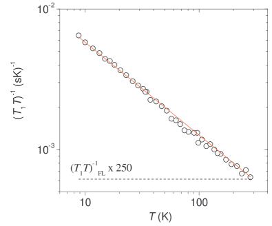
Figure 1: The temperature normalized NMR relaxation rate in SWCNTs at 3 T (symbols) from Ref. Ihara et al. (2010) fitted with the TLL model (solid line). The relaxation rate calculated in a Fermi-liquid picture, $(T_{1}T)^{-1}_{\text{FL}}$ (dashed line), is shown multiplied by a factor of 250.

The present theory of the NMR relaxation rate allows to compare it quantitatively with the experiment. In Fig. 1., we show the experimental NMR relaxation rate in SWCNTs at 3 T from Ref. Ihara et al. (2010). A fit with the above model in Eq. (5) gave $A_{\text{eff}}=3.6\cdot 10^{-7}\,\text{eV}$ when we fixed $K=1.34$ as in Ref. Ihara et al. (2010) and the DOS to the first principles based value of $\rho=0.007\,\text{states}/(\text{eV}\cdot\text{atom}\cdot\text{spin})$. This value of the effective hyperfine coupling is in good agreement with the literature values for other carbonaceous materials shown in Table. LABEL:ParameterTable.

The NMR line position also provides a measure of the HFC. For a TLL with anisotropic HFC, the Knight shift, ${\bf S}_{i}$ ($i=x,y,z$), reads:

$$S_{i}=A_{ii}\frac{\gamma_{e}}{2\gamma_{{}^{\text{C}}}}\rho K_{s},$$ (7)

where the $A_{ii}$’s are the diagonal elements of the HFC tensor. Eq. (7) retains the FL result for SWCNTs since therein $K_{s}=1$. For the powder SWCNT samples, the first moment of the NMR line is $A_{\text{iso}}$. The NMR data in Ref. Simon et al. (2005) gives an upper limit of 20 ppm for the isotropic Knight shift which leads to $A_{\text{iso}}<2.2\cdot 10^{-6}\,\text{eV}$ with the $\rho$ values in Table LABEL:ParameterTable. We note that first principles calculations by Yazyev gave an isotropic shift of 2 ppm for a (10,10) SWCNT, which corresponds to $A_{\text{iso}}=2.2\cdot 10^{-7}\,\text{eV}$.

We now turn to discuss the transport experiments on a double quantum dot (DQD) formed of ¹³C enriched SWCNTs Churchill et al. (2009), which found the HFC as large as $A=1-2\cdot 10^{-4}\,\text{eV}$ in marked contrast to the above value of $A_{\text{eff}}\simeq 10^{-6}\,\text{eV}$ obtained from the NMR data. The possibility to obtain the HFC from transport measurements on DQDs arises from the fact that the weak nuclear fields enable otherwise forbidden tunneling currents between the two dots, an effect called lifting of spin-blockade (LSB) Ono et al. (2002); Koppens et al. (2005a). This effect is now well established in GaAs quantum dots with a theory provided by Jouravlev and Nazarov (JN) Jouravlev and Nazarov (2006). In Ref. Churchill et al. (2009), the LSB was observed for the ¹³C enriched SWCNTs and a quantitative analysis was performed with a direct application of the JN theory. We discuss herein the essentials of the theory and present a potential alternative interpretation of the experimental results.

The JN theory starts by pointing out that the electron feels a ”frozen” nuclear field in each dot since the nuclear relaxation times are much longer than any relevant time scale for electrons. This condition remains valid for SWCNTs. The nuclear field in each dots is treated as a classical variable with values of ${\bf B}_{N}^{L}$ and ${\bf B}_{N}^{R}$ (for the left and right dots) with a Gaussian distribution Merkulov, I. A. and Efros, Al. L. and Rosen, M. (2002): $\langle({\bf B}_{N}^{L(R)})^{2}\rangle_{G}=B_{\rm N}^{2}$. Here, $g\mu_{\text{B}}B_{\rm N}=AI/\sqrt{N}$ with $g\approx 2$ being the electron $g$-factor, $\mu_{\rm B}$ is the Bohr magneton, and $N$ is the number of ¹³C nuclei in each dot Jouravlev and Nazarov (2006); Erlingsson, S. I. and Nazarov, Y. V. (2002).

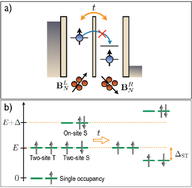
Figure 2: a) Schematics of a DQD; the contact leads (grey areas) and the internal hyperfine fields in the left and right dots are indicated. b) Energy levels for the DQD. Note that the tunneling parameter couples the on-site S and two-site S states and results in the singlet-triplet splitting.

Fig. 2a. shows the geometry and the energy structure of a DQD. The energy spectrum of the DQD consists of a ground state with single occupancy, followed by a doubly occupied two-site state (either singlet or triplet, separated by an energy $E$) and an on-site singlet state (S) (separated by $E+\Delta$), and finally an even higher lying on-site triplet state. Assuming an electron with spin up trapped in the right dot, only an electron with down spin can hop from the left side to this dot forming the on-site singlet state because spin-flip transitions are forbidden and the high energy on-site triplet state is not realized. Thus, for the two-dot system, two-electron spin singlet and triplet states can be identified. For the earlier, the transport is possible, whereas it is blocked for the latter. These states are separated by a singlet-triplet splitting, $\Delta_{\rm ST}$ End (c).

Without external magnetic and nuclear fields, $\Delta_{\rm ST}$ is determined by $\Delta$ and the interdot tunneling matrix element $t$: assuming large detuning $\Delta\gg t$, one finds $\Delta_{\rm ST}\approx t^{2}/\Delta$. Lifting of spin-blockade occurs when the difference of the nuclear fields between the two quantum dots, ${\bf B}_{\rm N}^{L}-{\bf B}_{\rm N}^{R}$, mixes the two-electron singlet and triplet states, which allows for a leakage current through the DQD.

The leakage current $I(B)$ through an SWCNT DQD as function of an external magnetic field $B$ was measured by Churchill et al. Churchill et al. (2009). Their data (Fig. 3f in Churchill et al. (2009)) shows a zero-field peak with width of $\sim 6\ {\rm mT}$. From the peak width the authors infer the HFC strength as $A=1-2\times 10^{-4}\,{\rm eV}$, using the JN theory that predicts that the peak width is proportional to the HFC if large detuning ($\Delta\gg t$), large nuclear fields ($B_{N}\gg\Delta_{\rm ST}$), and the dominance of inelastic (e.g. phonon-mediated) interdot tunneling are assumed.

We wish to draw attention to a potential alternative interpretation of the zero-field peak of $I(B)$ found in Churchill et al. (2009), which does not invoke the assumption of large nuclear fields. By analyzing the JN model in the regime of large detuning $\Delta\gg t$, but small nuclear fields $B_{N}\ll\Delta_{\rm ST}$ and no inelastic interdot tunneling, we find that the functional form of $I(B)$ is approximately a Lorentzian,

$$I(B)\sim\frac{B^{2}_{N}}{t^{2}}\frac{\gamma^{2}}{\gamma^{2}+B^{2}}e\Gamma_{R},$$ (8)

where $e$ is the electron charge, and $\Gamma_{R}$ is the tunneling rate of electrons from the on-site singlet state to the right lead. Most importantly, the width of the Lorentzian in Eq. (8) is obtained as $\gamma=\sqrt{3/8}\,\Delta_{\rm ST}$, i.e. it is independent of the HFC in contrast to the original analysis in Ref. Churchill et al. (2009). Derivation and discussion of Eq. (8) is provided in Sup .

We finally note that theoretical efforts focused on understanding the anomalously large HFC in the transport measurement and found the possibility of an increased HFC in TLL systems but limited to the millikelvin temperature range Braunecker et al. (2009a, b).

In conclusion, we developed the theory of NMR spin-lattice relaxation time in a Tomonaga-Luttinger liquid which enabled to determine the electron-nucleus hyperfine coupling constant in carbon nanotubes. The value is in disagreement with that deduced from transport measurements in quantum dots made of ¹³C enriched SWCNTs. We have reanalyzed the latter experiment in a different regime of the JN theory, which cures this discrepancy.

Work supported by the Hungarian State Grants (OTKA) Nr. K72613 and CNK80991, by the Austrian Science Funds (FWF) project Nr. P21333-N20, by the European Research Council Grant Nr. ERC-259374-Sylo, by the Marie Curie Grants PIRG-GA-2010-276834 and PERG08-GA-2010-276805, and by the New Széchenyi Plan Nr. TÁMOP-4.2.1/B-09/1/KMR-2010-0002. BD acknowledges the Bolyai programme of the Hungarian Academy of Sciences. AK acknowledges the Magyary programme and the EGT Norway Grants.

I Supplementary information

II The hyperfine coupling constant for atomic carbon

The isotropic hyperfine coupling (HFC) is zero for a free carbon atom and the dipolar HFC for the $p_{z}$ orbital is: $A_{\text{dip}}=\mu_{0}/4\pi\cdot\hbar^{2}\gamma_{\text{e}}\gamma_{{}^{13}\text{C}}\cdot 1.7/a_{0}^{3}\approx 5.5\cdot 10^{-7}\,\text{eV}$, where $\mu_{0}$, $\gamma_{\text{e}}$, $\gamma_{{}^{13}\text{C}}$, and $\mu_{0}$ are the permeability of vacuum, the electron and nuclear gyromagnetic ratios, and Bohr radius, respectively.

III The first principles calculation of the density of states in single-wall carbon nanotubes

We performed density functional theory calculations with the Vienna ab initio Simulation Package (VASP) Kresse and Furthmüller” (1996) within the local density approximation to calculate the density of states for metallic nanotubes within a bundled sample of a typical Gaussian diameter distribution centered around 1.4 nm with a variance of 0.1 nm. The projector augmented-wave method was used with a plane-wave cutoff energy of 400 eV. The band structures were calculated with a large k-point sampling, and the density of states was calculated with a simple Green’s function based approach from the band structure with a self-made utility. The density of states at the Fermi level was then averaged for the tubes examined. The considered nanotubes were (9,9), (15,6), (10,10), (18,0) and (11,11), in order of increasing diameter. The averaged density of states at the Fermi level for these metallic tubes was found to be 0.014 states/$\textrm{eV}\cdot\textrm{atom}$, i.e. 0.007 states/$\textrm{eV}\cdot\textrm{atom}\cdot\textrm{spin}$.

Note, that only a small number of nanotubes was considered when taking the average for a bundled sample. This approximation was necessary due to the large computation time for chiral tubes in this diameter range. In order to check whether this approximation results in any significant error, we made a test calculation with the nearest neighbor tight binding model. We found that performing the average on only a few tubes results in negligible error as compared to taking the average on every tube between 1.3 and 1.5 nm. This is due to the weak chirality dependence of the density of states at the Fermi level.

IV Theory of the hyperfine lifted spin blockade in single-wall carbon nanotubes

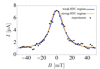
Figure 3: Comparison of experimental and theoretical results of the leakage current through a CNT DQD in the Pauli blockade setup. Points: measured current $I$ as the function of external axial magnetic field $B$ from Ref. Churchill et al. (2009). Solid blue line: fit of our theoretical result Eq. (13) [identical to Eq. (8) of the main text] corresponding to the weak-HFC parameter regime, with a $B$-dependent background current $I_{\rm bg}$ added. The parameters obtained from the fit: $\gamma=g\mu_{B}\times 10.4\ {\rm mT}$, $B_{N}^{2}e\Gamma_{R}/t^{2}\sim 6.4\ {\rm pA}$, and $I_{\rm bg}=0.84\ {\rm pA}$. Dashed orange line: the result Eq. (11) of Jouravlev and Nazarov (2006) with parameters $B_{N}=6.1$ mT, $\Gamma_{\rm in}=9.2$ pA, and a constant background current $I_{\rm bg}=1$ pA.

We describe the Pauli blockade effect using the model developed for GaAs double quantum dots (double QDs, DQDs) in Ref. Jouravlev and Nazarov (2006) End (d). Applying this model for carbon nanotube (CNT) DQDs is reasonable if short-range disorder in the CNT is sufficiently strong to destroy the valley degeneracy of the QD levels. Detailed analysis of the hyperfine coupling and Pauli blockade in valley-degenerate QDs are given in Refs Pályi and Burkard (2009, 2010).

We focus on the regime characterized by large detuning $\Delta\gg t$, weak HFC $B_{N}\ll\Delta_{\rm ST}$, and the absence of inelastic interdot tunneling, $\Gamma_{\rm in}=0$. Here $\Delta$ is the energy detuning between the two-site and on-site two-electron states , $t$ is the interdot tunneling amplitude, $B_{N}$ is the typical energy scale of the hyperfine interaction in one quantum dot, and $\Delta_{\rm ST}$ is the singlet-triplet energy splitting which, in this regime, is well approximated by $\Delta_{\rm ST}\approx t^{2}/\Delta$ (see Fig. 2 of main text). This regime has been treated in Jouravlev and Nazarov (2006), although no analytical formula was derived there for the leakage current averaged over the random Overhauser-field ensemble. Here we provide an analytical formula for the leakage current, based on a transparent physical picture, first-order perturbation theory and order-of-magnitude estimates.

In the regime of large detuning ($\Delta\gg t$), one of the five two-electron energy eigenstates is separated from the other four with an energy gap of $\sim\Delta$ and has a dominant on-site singlet character (see Fig. 2 of main text). As the wave function of this state is localized in the QD close to the drain contact, the state decays rapidly, with rate of $\sim\Gamma_{R}$, by emitting one electron to the drain and builds up slowly, with rate $\sim t^{2}\Gamma_{L}/\Delta^{2}$, as it is difficult to load an electron from the source to achieve this configuration. Therefore, this state plays a negligible role in the transport process.

In the absence of HFC, the remaining four energy eigenstates include one singlet state with dominantly two-site character and three two-site triplet states. The singlet and the triplets are energetically separated by $\Delta_{\rm ST}$. The exit rate of electrons from the singlet state is $\Gamma_{S}=(t/\Delta)^{2}\Gamma_{R}$, whereas triplet states are stationary. A magnetic field induces an energy splitting $B$ between the triplets while leaves the energy of the singlets unchanged. Random Overhauser fields in the two QDs induced by HFC couple triplets to the dominantly two-site singlet, with matrix elements typically on the order of $B_{N}$. The dominantly two-site singlet state has a nonzero decay rate $\Gamma_{S}$, therefore the electrons occupying the triplet states acquire finite exit rates:

$$\Gamma_{+} \sim \left(\frac{B_{N}}{\Delta_{\rm ST}-B}\right)^{2}\Gamma_{S},$$ (9)

$$\Gamma_{0} \sim \left(\frac{B_{N}}{\Delta_{\rm ST}}\right)^{2}\Gamma_{S},$$ (10)

$$\Gamma_{-} \sim \left(\frac{B_{N}}{\Delta_{\rm ST}+B}\right)^{2}\Gamma_{S}.$$ (11)

Here the Zeeman shift $B$ of the $T_{\pm}$ levels were taken into account in the energy denominators. Although the decay rate $\Gamma_{\pm}$ diverges at $B=\pm\Delta_{\rm ST}$ (which is an artifact of perturbation theory), this divergence is harmless regarding our result for the leakage current [see Eq. (13)] as that is insensitive of the rates of the fastest processes.

The leakage current is inversely proportional to the average time an electron spends in the DQD, which is

$$T_{\rm avg}=\frac{1}{4}\left(\Gamma_{S}^{-1}+\Gamma_{+}^{-1}+\Gamma_{0}^{-1}+\Gamma_{-}^{-1}\right)\approx\frac{1}{4}\left(\Gamma_{+}^{-1}+\Gamma_{0}^{-1}+\Gamma_{-}^{-1}\right),$$ (12)

which yields Eq. (8) of the main text:

$$I(B)=\frac{e}{T_{\rm avg}(B)}\sim\frac{B^{2}_{N}}{t^{2}}\frac{\gamma^{2}}{\gamma^{2}+B^{2}}e\Gamma_{R},$$ (13)

where $e$ is the electron charge, and the width of the Lorentzian is $\gamma=\sqrt{3/8}\,\Delta_{\rm ST}$, i.e., it is independent of the HFC.

As mentioned above, our result Eq. (13) is based on the model developed in Jouravlev and Nazarov (2006). To our understanding, the range of validity of Eq. (13) is the same as that of Eq. (6) of Jouravlev and Nazarov (2006). The difference between the two results is that the latter describes the leakage current $I(B)$ at a fixed Overhauser-field configuration, whereas the former estimates the functional form of $I(B)$ without referring explicitly to the Overhauser-field configuration. We have checked that numerical averaging of Eq. (6) of Jouravlev and Nazarov (2006) over random Overhauser-field configurations yields similar results as our Eq. (13).

Fig. 3 shows the experimental data together with the theoretical curve corresponding to the strong-HFC regime treated in Jouravlev and Nazarov (2006) and used originally to describe the CNT DQD experiment (dashed orange line), as well as our result Eq. (13) corresponding to the weak-HFC regime (solid blue line). Both theoretical curves fit the experimental data reasonably well. Note that it is not possible to infer the value of the Overhauser-field strength $B_{N}$ directly from the fit of our result to the data.

A characteristic feature observed in the experiment (see Fig. 3b in Churchill et al. (2009)) is the apparent symmetry of the leakage current upon changing the sign of the detuning $\Delta$, which seems to hold if $\Delta$ is between $\pm 0.6$ meV. Equation (13) is consistent with this feature as it depends only on $\Delta^{2}$. In contrast, in the strong-HFC regime of the theory Jouravlev and Nazarov (2006), the interdot tunneling is assumed to be inelastic, hence the corresponding rate $\Gamma_{\rm in}$ is expected to be very sensitive of the sign of $\Delta$ (slow energetically uphill transitions vs. fast downhill transitions) at low temperature Koppens et al. (2005b).

From the fit shown in Fig. 3, we deduce $\Delta_{\rm ST}\approx 2\ \mu$eV, if an electronic g-factor $g=2$ is assumed. Such a singlet-triplet splitting $\Delta_{\rm ST}$ is created if, e.g., $\Delta=10\ \mu$eV and $t=4.5\ \mu$eV. Taking these values, the value of the NMR-based atomic HFC $A=0.36\ \mu$eV, and assuming $N=3\times 10^{4}$ atoms in a QD (corresponding to $B_{N}\approx 2$ neV), from the fit we obtain $\Gamma_{R}\approx 3\times 10^{8}$ MHz. This corresponds to a level broadening $h\Gamma_{R}\approx 1$ eV. In a device showing QD characteristics it is expected that the level broadening is much smaller than the level spacing ($\sim 1$ meV in Churchill et al. (2009)). Therefore, although the qualitative agreement between the experiment and our theoretical result (13) is remarkable, the above estimate implies that our result is unable to quantitatively describe the experiment.

References

- Kane (1998) B. Kane, Nature 393, 133 (1998).
- Slichter (1989) C. P. Slichter, Principles of Magnetic Resonance (Spinger-Verlag, New York, 1989), 3rd ed.
- Žutić et al. (2004) I. Žutić, J. Fabian, and S. D. Sarma, Rev. Mod. Phys. 76, 323 (2004).
- Abragam (1961) A. Abragam, Principles of Nuclear Magnetism (Oxford University Press, Oxford, England, 1961).
- Perera et al. (1994) S. A. Perera, J. D. Watts, and R. J. Bartlett, J. Chem. Phys. 100, 1425 (1994).
- Ingram (1958) D. J. E. Ingram, Free Radicals as Studied by Electron Spin Resonance (Butterworths Scientific Publications, 1958).
- Pennington and Stenger (1996) C. H. Pennington and V. A. Stenger, Rev. Mod. Phys. 68, 885 (1996).
- Yazyev (2008) O. V. Yazyev, Nano Lett. 8, 1011 (2008).
- Mcmanus et al. (1988) H. J. Mcmanus, R. W. Fessenden, and D. M. Chipman, J. Phys. Chem. 92, 3781 (1988).
- Churchill et al. (2009) H. O. H. Churchill, A. J. Bestwick, J. W. Harlow, F. Kuemmeth, D. Marcos, C. H. Stwertka, S. K. Watson, and C. M. Marcus, Nat. Phys. 5, 321 (2009).
- Jouravlev and Nazarov (2006) O. Jouravlev and Y. Nazarov, Phys. Rev. Lett. 96, 176804 (2006).
- Van de Walle and Blöchl (1993) C. G. Van de Walle and P. E. Blöchl, Phys. Rev. B 47, 4244 (1993).
- Pályi and Burkard (2009) A. Pályi and G. Burkard, Phys. Rev. B 80, 201404(R) (2009).
- Tang et al. (2000) X.-P. Tang, A. Kleinhammes, H. Shimoda, L. Fleming, K. Y. Bennoune, S. Sinha, C. Bower, O. Zhou, and Y. Wu, Science 288, 492 (2000).
- Goze-Bac et al. (2001) C. Goze-Bac, S. Latil, L. Vaccarini, P. Bernier, P. Gaveau, S. Tahir, V. Micholet, and R. Aznar, Phys. Rev. B 63, 100302(R (2001).
- Singer et al. (2005) P. M. Singer, P. Wzietek, H. Alloul, F. Simon, and H. Kuzmany, Phys. Rev. Lett. 95, 236403 (2005).
- Ihara et al. (2010) Y. Ihara, P. Wzietek, H. Alloul, M. H. Rümmeli, T. Pichler, and F. Simon, Eur. Phys. Lett. 90, 17004 (2010).
- Bockrath et al. (1999) M. Bockrath, D. H. Cobden, J. Lu, A. G. Rinzler, R. E. Smalley, L. Balents, and P. L. McEuen, Nature 397, 598 (1999).
- Yao et al. (1999) Z. Yao, H. W. C. Postma, L. Balents, and C. Dekker, Nature 402, 273 (1999).
- Ishii et al. (2003) H. Ishii, H. Kataura, H. Shiozawa, H. Yoshioka, H. Otsubo, Y. Takayama, T. Miyahara, S. Suzuki, Y. Achiba, M. Nakatake, et al., Nature 426, 540 (2003).
- Rauf et al. (2004) H. Rauf, T. Pichler, M. Knupfer, J. Fink, and H. Kataura, Phys. Rev. Lett. 93, 096805 (2004).
- Tomonaga (1950) S. Tomonaga, Prog. Theor. Phys. 5, 349 (1950).
- Luttinger (1963) J. M. Luttinger, J. Math. Phys. 4, 1154 (1963).
- Dóra et al. (2007) B. Dóra, M. Gulácsi, F. Simon, and H. Kuzmany, Phys. Rev. Lett. 99, 166402 (2007).
- Gao et al. (2004) B. Gao, A. Komnik, R. Egger, D. C. Glattli, and C. Bachtold, Phys. Rev. Lett. 92, 216804 (2004).
- End (a) A factor 4 appears in Eq. (2) if the DOS is defined as .
- End (b) We note that Ref. Tang et al. (2000) cites a value from Ref. Mintmire and White (1998) that is a factor 2 larger due to neglect of the spin degeneracy.
- (28) See EPAPS Document No. XXX for supplementary material providing further technical details.
- Mintmire and White (1998) J. Mintmire and C. White, Phys. Rev. Lett. 81, 2506 (1998).
- Voit (1995) J. Voit, Rep. Prog. Phys. 58, 977 (1995).
- Simon et al. (2005) F. Simon, C. Kramberger, R. Pfeiffer, H. Kuzmany, V. Zólyomi, J. Kürti, P. M. Singer, and H. Alloul, Phys. Rev. Lett. 95, 017401 (2005).
- Ono et al. (2002) K. Ono, D. G. Austing, Y. Tokura, and S. Tarucha, Science 297, 1313 (2002).
- Koppens et al. (2005a) F. H. L. Koppens, J. A. Folk, J. M. Elzerman, R. Hanson, L. H. W. van Beveren, I. T. Vink, H. P. Tranitz, W. Wegscheider, L. P. Kouwenhoven, and L. M. K. Vandersypen, SCIENCE 309, 1346 (2005a).
- Merkulov, I. A. and Efros, Al. L. and Rosen, M. (2002) Merkulov, I. A. and Efros, Al. L. and Rosen, M., Phys. Rev. B 65, 205309 (2002).
- Erlingsson, S. I. and Nazarov, Y. V. (2002) Erlingsson, S. I. and Nazarov, Y. V., Phys. Rev. B 66, 155327 (2002).
- End (c) This is not to be mistaken with the singlet-triplet gap for a doubly occupied QD.
- Braunecker et al. (2009a) B. Braunecker, P. Simon, and D. Loss, Phys. Rev. B 80 (2009a).
- Braunecker et al. (2009b) B. Braunecker, P. Simon, and D. Loss, Phys. Rev. Lett. 102 (2009b).
- Kresse and Furthmüller” (1996) G. Kresse and J. Furthmüller”, Phys. Rev. B 54, 11169 (1996).
- End (d) Magnetic field is used in energy units throughout.
- Pályi and Burkard (2010) A. Pályi and G. Burkard, Phys. Rev. B 82, 155424 (2010).
- Koppens et al. (2005b) F. H. L. Koppens, J. A. Folk, J. M. Elzerman, R. Hanson, L. H. W. van Beveren, T. Vink, H. P. Tranitz, W. Wegscheider, L. P. Kouwenhoven, and L. M. K. Vandersypen, Science 309, 1346 (2005b).