Kinematic dynamo simulations of von Kármán flows: application to the VKS experiment

Abstract

The VKS experiment has evidenced dynamo action in a highly turbulent liquid sodium von Kármán flow [R. Monchaux et al., Phys. Rev. Lett. 98, 044502 (2007)]. However, the existence and the onset of a dynamo happen to depend on the exact experimental configuration. By performing kinematic dynamo simulations on real flows, we study their influence on dynamo action, in particular the sense of rotation and the presence of an annulus in the shear layer plane. The 3 components of the mean velocity fields are measured in a water prototype for different VKS configurations through Stereoscopic Particle Imaging Velocimetry. Experimental data are then processed in order to use them in a periodic cylindrical kinematic code. Even if the kinematic predicted mode appears to be different from the experimental saturated one, the results concerning the existence of a dynamo and the thresholds are in qualitative agreement, showing the importance of the flow characteristics.

I Introduction

Dynamo action is an instability by which mechanical energy is transformed into magnetic energy for $R_{m}\geq R_{m}^{c}$ where $R_{m}$ is the magnetic Reynolds number. Since Larmor’s prediction concerning the solar dynamoLarmor , a lot of work has been devoted to this field, including both theories and numerical simulations. In the last decade, the interest for dynamo has been renewed by the positive results obtained by the Riga G01 and Karlsruhe SM01 fluid dynamo experiments. These experiments rely on analytical predictions by Ponomarenko Pono and Robert GORoberts and have been designed accordingly. In particular, the generated turbulent sodium flows are organized so that the instantaneous flow remains always close to the mean flow, allowing the kinematic dynamo predictions of the thresholds and of the neutral modes (respectively oscillatory and stationary) to be very accurate.

A new step was passed very recently in the von Kármán Sodium (VKS) experiment. Different dynamos have been observed inside a flow of liquid sodium at large Reynolds number ($Re\sim 10^{7}$) MBB07 ; BMF07 ; P3 ; P5 . Depending on the the control paramaters, statistically stationary dynamos or dynamical dynamo regimes including field reversals have been reported. Under these conditions, the flow is fully turbulent, with many large and small scale fluctuations, and the instantaneous flow is very different from the mean flow RCD08 ; CDM09 . The dynamo instability taking place in the VKS experiment is thus at variance with the classical instabilities taking place in laminar flows or in turbulent flows remaining very close to their mean. Nevertheless, many kinematic dynamo simulations have been performed to optimize this flow, using the synthetic MND flow MND06 or time-averaged flows measured in water-prototype experiments MBD03 ; RCD05 ; SXG06 .

Different observations have been made that can help elucidate the exact mechanism by which the dynamo instability develops in the VKS experiment: i) in the exactly counter-rotating case, dynamo action is observed above a critical magnetic Reynolds number $R_{m}^{c}\approx 32$ and the dominant saturated mode is an axisymmetric m=0 mode in cylindrical coordinates MBB07 ; ii) so far, dynamo has only been observed with iron propellers P5 ; iii) in a given experimental set up with iron disks, dynamo has been observed when counter-rotating disks in (+) ’non scooping’ direction (with respect to the propellers blades), but no dynamo has been observed when counter-rotating the disks in the (-) ’scooping’ direction P5 .

Observation i) shows that the dynamo mechanism is not the simple linear response to the mean flow alone, since the latter is axisymmetric and produces a transverse $m=1$ mode ($m$ denotes the azimuthal wavenumber) above $R_{m}^{c}\simeq 43$ as indicated by kinematic dynamo simulations RCD05 . It has been suggested in GAFDFauve that the m=0 mode of the VKS experiment is in fact generated by non-axisymmetric fluctuations through an alpha-omega mechanism taking place within the blades of the propellers. This suggestion has been confirmed by recent numerical simulations LNRLGP08 showing that the addition of an (empirical and large) alpha term in the induction equation changes the dominant m=1 mode into a dominant m=0 mode with a dynamo threshold close to the observed experimental critical value $R_{m}^{c}\approx 32$. Another interesting suggestion has been made by GDF08 , namely that the m=0 mode could arise from a secondary bifurcation of the m=1 mode, since the latter breaks the original axisymmetry of the velocity field.

Observation ii) shows that magnetic boundary conditions have a large impact on the dynamo instability. High magnetic permeability conditions are known to decrease the dynamo threshold for the Roberts and Ponomarenko flows APG03 and more recently for von Kármán type flows GIFD08 . For iron disk, it is suggested that the dynamo threshold could be reduced by a factor as large as 2 with respect to stainless disks. Since it has not been yet possible to get beyond $R_{m}=50$ in the VKS experiment, this could explain why dynamo has not been observed with stainless steel disks, while it is observed around $R_{m}=32$ with iron disks. Other kinematic simulations SXG06 have shown that the sodium flow behind the disks can lead to an increase from $12\%$ to $150\%$. Using iron disks can thus also screen magnetic effects of the flow behind the disks. PARLER des DISQUES CAMEMBERTS?

Observation iii) shows that the dynamo is not produced only by the rotation of magnetized iron disks in a conducting fluid but depends on the flow characteristics: it is a real fluid dynamo. However, not much has been done so far to try and exploit this observation. In particular, no kinematic dynamo simulations have been performed so far with experimental flows including an annulus as in the VKS experiment or with propellers counter-rotating in the (-) ’scooping’ direction.

In the present paper, we use Stereoscopic Particle Imaging Velocimetry (SPIV) measurements obtained in von Kármán water (VKE) experiments modeling the VKS experiment to perform kinematic dynamo simulations. We investigate the role of the mean field structure on the dynamo threshold, with special attention to the rotation sense. Because of the axisymmetry, the exhibited kinematic mode is, as expected, different from the experimental saturated one. However, we show that the kinematic dynamo thresholds qualitatively vary like the observed dynamo thresholds and discuss how these results can be useful to understand the actual mechanisms at the origin of VKS dynamo.

Our paper is organized as follows: In Sec. II, after the problem formulation, we describe the experimental measurements and the numerical method. In Sec. III, we focus on the processing procedure of the measured velocities and perform a comparison with previous estimates based on Laser Doppler Velocimetry (LDV) measurements. Results for dynamo action are presented in Sec. IV and compared with the VKS experiments. Finally, we discuss the consequences of these results for the VKS dynamo.

II Methods

II.1 Problem Formulation

In the present paper, we focus on the kinematic dynamo problem: we consider a given velocity field $\mathbf{u}$, e.g. as measured in a water experiment, and check its ability to sustain dynamo action by solving the magnetic induction equation

$$\frac{\partial\mathbf{b}}{\partial t}=\nabla\times\left(\mathbf{u}\times\mathbf{b}\right)+\frac{1}{\mu\sigma}\triangle\mathbf{b},$$ (1)

where $\mathbf{b}$ denotes the magnetic field with $\nabla\cdot\mathbf{b}=0$, $\mu$ and $\sigma$ are respectively the magnetic permeability and the electrical conductivity of the considered medium, and $\Delta$ is the Laplacian operator. Since $\mathbf{u}$ is given, the equation is linear in $\mathbf{b}$. There are two possible long-time behaviour for the magnetic field: either it is decaying and there is no dynamo, or it is increasing, and there is dynamo. Growth or decay is in general exponential (although there can be transient algebraic growth, due to non-normality of the operator, see LJ06 ). To quantify the growth, we introduce the growth rate $\sigma=\partial_{t}\ln\left<B^{2}\right>$ that is based on the magnetic energy $\left<B^{2}\right>$, where the average is taken over the spatial domain.

Since the equation is linear, no saturation is observed in the kinematic approach. This technique is therefore unable to detect subcritical or finite amplitude dynamos PLD07 or to study the saturation regime PMM05 ; LBL06 ; DBM07 as in numerical flows such as the Taylor-Green flow.CITER SIMULATIONS FOREST??. However, this approach gives an estimation for the dynamo threshold as a function of the mean velocity field.

II.2 Experimental measurements

Geometry and experimental setup.— The setup corresponding to the VKS experiment is described in details in MBB07 and sketched in Figure 1(a). A cylindrical vessel with a fixed aspect ratio of $L=H/R=1.8$, where $R$ (resp. $H$) denotes the radius (reps. the length) of the vessel which is filled with liquid sodium. We arrange the coordinate system such, that the axial extension of the cylinder is situated in the interval $z\in[-0.9,0.9]$. The fluid is stirred by two independent rotating so called TM73 impellors RCD05 , at frequencies $f_{1}$ and $f_{2}$. The impellers are fitted with curved blades (see Fig. 1 (b)). Therefore, the flow properties depend on the sense of rotation, specifically on whether the blades are presenting their concave ((-) rotation) or convex ((+) rotation) side to the flow during impeller rotation. In the special case where $f_{1}=f_{2}>0$ (resp. $f_{1}=f_{2}<0$) with the sign convention of Fig. 1, the impellers fullfill exact (+) (resp. (-)) counter-rotation. An optional concentric annulus can also be inserted at mid height and has been used in the first dynamo runs. This annulus reduces large scale fluctuations CDM09 and can also have an impact on the mean flow, in particular on the toroidal to poloidal ratio $\Gamma$ (see below). In the VKS experiment, an additional layer of resting sodium is present in the outer part of the experiment.

The VKE experiment is the exact half-scale water model of the VKS experiment, except that the experiment is realized vertically (vertical z axis) whereas the VKS setup is horizontal. The cylinder radius and height of the VKE vessel are $R=100$ and $240$ mm respectively. We have used TM73 impellers of diameter $150$ mm fitted with radial blades of height $20$ mm and curvature radius $92.5$ mm. The inner faces of the disks are $H=180$ mm apart. We have worked with different vessel geometries, allowing the insertion of an annulus - thickness $5$ mm, inner diameter $170$ mm - in the equatorial plane. Note also that in the VKE experiment, the layer of resting fluid is absent. The velocity field is therefore only measured in the flow region, see Fig. 1 (a).

Velocity measurements are performed using a DANTEC SPIV system, providing the three components of the velocity field on a plane through a $95\times 66$ points grid M07 . In all that follows, the measurement plane is a meridian plane containing the rotation axis. The velocity fields are averaged over time series of $5000$ regularly sampled values (sampling frequency between 1 and 15 Hz). In the exact counter-rotating regime, the system is axisymmetric and symmetric with respect to any rotation $R_{\pi}$ of $\pi$ around any radial axis in its equatorial plane. The mean flow is composed of two toroidal cells separated by an azimuthal shear layer and two poloidal recirculation cells. Figure 2 shows the velocity fields obtained in the 4 studied configurations: (+) and (-) rotation sense in the presence or the absence of an annulus in the equatorial plane. Note that in the exact counter-rotating regime, no turbulent bifurcation towards a one cell state is observed with the TM73 impellers contrary to what is reported for impellers with higher curvarture blades in RMC04 . The bifurcation is observed in the (+) sense for a rotation number $\theta=(f_{1}-f_{2})/(f_{1}+f_{2})=0.1$ without annulus and $\theta=0.17$ with annulus CDM09 .

Control parameters.— Choosing the magnetic field diffusion time $\mu\sigma R^{2}$ as the time scale, and the maximum absolute value of the flow velocity $|\mathbf{u}|_{\textrm{max}}$ as velocity unit, the induction equation can be expressed in dimensionless form:

$$\frac{\partial\mathbf{b}}{\partial t}=R_{m}\nabla\times\left(\mathbf{u}\times\mathbf{b}\right)+\triangle\mathbf{b},$$ (2)

where $R_{m}=\mu\sigma R|\mathbf{u}|_{\textrm{max}}$ is the magnetic Reynolds number. The critical magnetic Reynolds number $R_{m}^{c}$ for dynamo onset is then defined such that $\sigma(R_{m}^{c})=0$. Another important parameter to characterize the velocity field is the poloidal to toroidal ratio:

$$\Gamma = \frac{\left<P\right>}{\left<T\right>},\ \textrm{with}$$ (3a)

$$\left<P\right> = \int_{-L/2}^{L/2}dz\int_{0}^{1}\sqrt{u_{r}(r,z)^{2}+u_{z}(r,z)^{2}}rdr,$$ (3b)

$$\left<T\right> = \int_{-L/2}^{L/2}dz\int_{0}^{1}\left|u_{\Theta}(r,z)\right|rdr,$$ (3c)

which is known to have a great impact on the dynamo threshold MBD03 ; RCD05 . Here we denoted the components of the velocity field in cylindrical coordinates as $\mathbf{u}=(u_{r},u_{\Theta},u_{z})$.

II.3 Numerical code

Because the system is axisymmetric, the time-averaged velocity field is supposed to be axisymmetric. We integrate the induction equation using an axially periodic kinematic dynamo code. We only provide here its brief description, details can be found in L94 . The code is pseudospectral in the axial and azimuthal directions while the radial dependence is treated by a high-order finite difference scheme. The numerical resolution corresponds to a grid of $81$ points for one wavelength in axial direction, $4$ points in azimuthal direction (corresponding to azimuthal wave numbers $m=0,\pm 1$) and $31$ points in radial direction for the flow domain. The time scheme is second-order Adams-Bashforth with a typical time step of $10^{-5}$.

Electrical conductivity and magnetic permeability are homogeneous and the external medium is insulating. Implementation of the magnetic boundary conditions for a finite cylinder is difficult, due to the nonlocal character of the continuity conditions at the boundary of the conducting fluid GIFD08 . In contrast, axially periodic boundary conditions are easily formulated, since the harmonic external field then has an analytical expression. Indeed, the numerical elementary box consists of two mirror-symmetric experimental velocity fields in order to avoid strong velocity discontinuities along the $z$ axis RCD05 . Note that we do not take into account the effet of the flow behind the propellers. This effect has been studied in details in other kinematic simulations SXG06 .

Finally, we can act on the electromagnetic boundary conditions by adding a layer of stationary conductor of dimensionless thickness $w$, corresponding to sodium at rest surrounding the flow exactly as in the VKS experiment in Cadarache MBB07 . This extension is made keeping the radial resolution of the experimental measured velocity field constant ($31$ points in the flow region). The velocity field we use as input for the numerical simulations is thus simply fit in an homogeneous conducting cylinder of radius $1+w$:

$$\mathbf{u} = \mathbf{u}_{\textrm{flow}}\quad\textrm{for}\quad 0\leq r\leq 1,$$ (4a)

$$\mathbf{u} = 0\quad\textrm{for}\quad 1<r\leq 1+w.$$ (4b)

Former investigations RCD05 showed a decrease of the critical magnetic Reynolds number for increasing conducting layer size, with a saturation above $w=0.4$. Therefore, we fixed $w=0.4$ (meaning altogehter $43$ points in radial direction) in order to save computing time. Some calculations with $w=0.6$ ($49$ points) have also been done, when comparing with older computations based on LDV measurements.

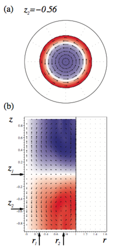
Figure 3: Same as in Figure 2: (+) rotation has been used and there is no annulus. Part (a) indicates a section for fixed $z=z_{2}=-0.56$, whereas in (b) an arbitrary cut of the rotational invariant field for fixed $\Theta$ is displayed. The arrows in (b) illustrate the section planes for the profiles shown in figures 4 and 5.

Figure 3 gives an example of the total velocity field used in kinematic simulations, consisting of an experimentally measured velocity field $\mathbf{u}_{\textrm{flow}}$ and a conducting layer with $w=0.6$.

III Data preparation and tests

III.1 Preparation of measured velocities

Due to experimental measurement constraints, it is impossible to determine the field in the whole cylinder cut $(r,z)=\left([0,1],[-0.9,0.9]\right)$: i) in the propeller regions, the presence of blades prevents the SPIV measurements; ii) close to the cylinder, reflection effects spoil any velocity measurements; iii) when an annulus is inserted at mid-height ($z=0$), measurements cannot be performed in the thin area behind and around the annulus. Therefore a typical data set covers only the area $(r,z)\approx\left([0,0.9],[-0.6,0.6]\right)$. This means, that approximately more than a third of the velocity field is unknown and has to be determined by boundary conditions and spline extrapolation. The radial adaptation has always been performed before the axial one. The preparation methods of the used SPIV measurements are explained in detail in the following.

Axial Symmetrization.— For the perfect counter-rotating setup an axial symmetrization has been performed with height mid as reflection plane. After this procedure $u_{r}$ is strictly symmetric, whereas $u_{\Theta}$ and $u_{z}$ are antisymmetric.

Axial boundary conditions.— The axial velocity field should vanish at the blade border, therefore we imposed the condition $u_{z}(z=\pm 0.9)=0$. The two other components fullfill a vanishing derivative in axial direction at the blades, meaning $\partial u_{\Theta}/\partial z(z=\pm 0.9)=0$ and $\partial u_{r}/\partial z(z=\pm 0.9)=0$.

Extrapolation in axial direction.— Close to the blades the fields are unknown and even not all the data which are measured are suitable, meaning that inappropriate values have to be removed. This lack is repaired by a spline extrapolation. The aforementioned boundary conditions help us to implement a good fit. The procedure at the top and the bottom blade is the same. The number of points which have to be removed at a blade are denoted by nrp (=“number of removed points”) in the following text. We compared results for different values of nrp in order to find a trustable result with a respective error estimate. Altogether between 11 and 15 points have to be extrapolated at a blade corresponding to a nrp between $2$ and $6$, meaning that for the first $9$ points no measured values are available. The number of points used to determine the spline function has no significant influence on the result, as far as more than $3$ are taken into account. For security reasons we always took $6$ points.

Interpolation in the annulus region.— When the annulus is present, there are typically $8$ (10 % of the data set) measured points around the mid-height that are absent or spoiled. They have been removed and replaced by spline interpolated values, which is a good natured operation.

Radial boundary conditions.— The radial velocity field vanishes at the cylinder border, therefore we imposed the condition $u_{r}(r=1)=0$. The two other components satisfy $\partial u_{\Theta}/\partial r(r=1)=0$ and $\partial u_{z}/\partial r(r=1)=0$. In the cylinder center the radial and azimuthal components are zero, meaning $u_{r}(r=0)=u_{\Theta}(r=0)=0$, whereas the axial field has a disappearing derivative $\partial u_{z}/\partial r(r=0)=0$.

Extrapolation in radial direction.— Close to the cylinder the last two points have been replaced and an additional point has been added to reach the cylinder border. They are the result of a spline extrapolation fullfilling the aforementioned boundary conditions using two points for the function construction.

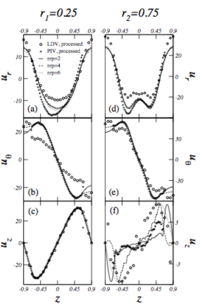
Figure 4: Profiles of the velocity fields in cylindrical coordinates $\mathbf{u}=(u_{r},u_{\Theta},u_{z})$ for fixed radii as explained in Fig. 3. A setup with (+) rotation has been used and there is no annulus. The left (right) column shows a section far away (nearby) the vortex center. Data obtained by processed LDV RCD05 (circles) are compared with SPIV measurements (crosses). The lines show processed SPIV data used in the kinematic dynamo code for different spline extrapolation procedures, see text for details. All fields are in arbitrary units and scaled to the maximal amplitude of the LDV data for comparison reasons. Note that in part (f) the the scaling is expanded and the SPIV data values are very small.

Check with LDV measurements.— LDV measurements are free of certain deficiency of the SPIV measurements, especially near the cylinder boundary, where reliable velocity fields can be obtained. It is therefore interesting to test the validity of our SPIV field preparation by comparison with LDV fields obtained previously by Ravelet et al. RCD05 . Figure 4 compares the velocity fields of LDV with the new SPIV measurements for fixed radial coordinate cuts explained in Fig. 3. One cut is close to the vortex center, the other one far away. A setup with (+) counter rotation has been used without annulus. In addition, the processed data, used in the code, with the aid of symmetrization and spline extrapolation for different nrp are shown. The difference between the two curves is mainly in the azimuthal field $u_{\Theta}$ nearby the blades. Note, that the large deviations of the two processed curves for the $u_{z}$ field in the regime $r\approx[-0.6,0.6]$ is only due to the performed scaling described in the caption. The SPIV dataset is finer and overall the comparison is quite satisfactory.

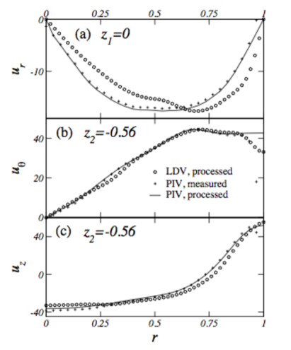
Figure 5: Profiles of the velocity fields in cylindrical coordinates $\mathbf{u}=(u_{r},u_{\Theta},u_{z})$ for fixed axial heights as explained in Fig. 3 and in caption of Fig. 4. (+) rotation has been used and there is no annulus. For these cuts (far away from the blades) there is no difference in the different spline extrapolations. Fields are shown in planes capturing their maximal value: (a) $u_{r}$ in the inflow area separating the vortex pair at $z=z_{1}=0$; (b) and (c) $u_{\Theta}$ and $u_{z}$ in the vortex center at $z=z_{2}=-0.56$. Data obtained by processed LDV RCD05 (circles) are compared with SPIV measurements (crosses) and processed data (line).

Corresponding cuts for fixed axial coordinate are shown in Fig. 5 for planes in the vortex region and in the pure inflow layer separating the vortex pair. The agreement between LDV and SPIV measurements is good even if a small deviation can be observed on $u_{r}$.

AJOUTER PHRASE CONCLUSION: AVANTAGE SPIV/LDV

III.2 Influence of the annulus

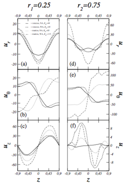
Figure 7: Comparison of the profiles of the velocity fields corresponding to the 4 studied configurations for fixed radii as explained in Fig. 3: (+) rotation without annulus (continuous line); (+) rotation with annulus at mid height (dashed line); (-) rotation without annulus: artificial numerical field with $\Gamma=0.8$ (dotted line); (-) rotation with annulus at mid height (dashed-dotted line)

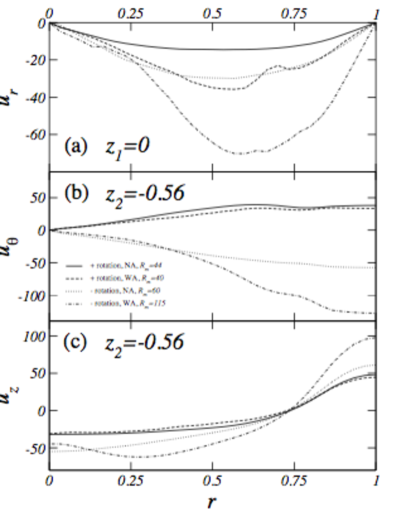
Figure 8: Comparison of the profiles of the velocity fields corresponding to the 4 studied configurations for fixed axial height as explained in Fig. 3: (+) rotation without annulus (continuous line); (+) rotation with annulus at mid height (dashed line); (-) rotation without annulus:: artificial numerical field with $\Gamma=0.8$ (dotted line); (-) rotation with annulus at mid height (dashed-dotted line)

In order to study the influence of the annulus, we have measured the corresponding time-averaged velocity field for different nrp (cf. Fig. 6). The velocity fields corresponding to the 4 configurations that are used in the kinematic dynamo simulations are then shown in Figures 7 and 8.

In the (+) rotation case, the axial gradient of $u_{r}$, $u_{\theta}$ and $u_{z}$ are larger in the region of the shear layer. The variation with $r$ of the velocity fields looks very similar except for $u_{r}$ at mid-radius. However, the poloidal to toroidal ratio $\Gamma$, does not reflect this difference: $\Gamma=0.8$ in both cases.

In the (-) rotation case, we were not able to perform such a detailed comparison, due to an unexpected experimental problem: the locking of large scale vortices of the middle shear layer at the position of the small cut performed through the annulus to enable SPIV measurements (cf. CDM09 for details). This locking does not occur in the (+) case, resulting in an axisymmetric time-averaged velocity field. In the (-) rotating case, however, the locking artificially breaks the axisymmetry of the time-averaged field, preventing a priori the comparison with the case without annulus. Computation of $\Gamma$ reveals a difference between the left ($\Gamma=0.89$) part of the SPIV plane where the vortices are trapped and the right ($\Gamma=0.62$) part where there is no trapping. Other measurements show that only this right part is relevant for the VKS experiment in which the annulus is cut-free. In the following, we use this right part and symmetrize the velocity field accordingly. The corresponding $\Gamma$ in (-) rotation sense are thus $0.62$ with annulus, and $0.49$ without annulus.

To see the influence of $\Gamma$ on dynamo action for these velocity fields, we have also built a synthetic velocity field by taking the velocity field measured in the (-) rotation case without annulus, and rescaling its poloidal components to reach $\Gamma=0.8$. This synthetic field is represented in Fig. 7 and 8. The variations of its velocity components with $z$ and $r$ are very similar to those obtained for the (+), contary to the variation of the (-) case with annulus.

III.3 Test of the code and the preparation method

Several kinds of tests have been performed in order to check the numerical code as well as the preparation methods of the SPIV data described in section III.1.

Ohmic diffusion.— The magnetohydrodynamic equations (2) reduce for vanishing velocity field $(\mathbf{u}=0)$ to the ohmic diffusion equation in cylindrical geometry

$$\frac{\partial\mathbf{b}}{\partial t}=\triangle\mathbf{b},$$ (5)

which has analytical eigenfunctions consisting of Bessel functions MND06 . We imposed these eigenfunctions in the code with a subsequent monitoring of the exponential decay of the amplitude. In all the investigated cases the theoretical eigenvalue has also been observed in the numerical run with high accuracy.

Comparison with analytical flow results.— We used also the MND flow, an analytical velocity field studied in MND06 in order to ckeck our code. For the field given by:

$$u_{r} = -\frac{\pi}{2}r(1-r)^{2}(1+2r)\cos(\pi z),$$ (6a)

$$u_{\Theta} = (1-r)(1+r-5r^{2})\sin(\pi z/2),$$ (6b)

$$u_{z} = 4\epsilon r(1-r)\sin(\pi z),$$ (6c)

with aspect ratio $L=2$, for $\Gamma=0.776$ and $\epsilon=0.743$, the expected critical magnetic Reynolds number is $58$, which we could confirm with our code.

Comparison with LDV data.— In order to check our preparation procedure of the SPIV measurements we compared also our computations with former LDV results presented in RCD05 . The used fields have already been presented in figures 4 and 5 for a (+) rotating setup without annulus. Therefore we computed for different nrp values, namely $2,4$ and $6$, the magnetic energy growth rate as a function of $R_{m}$. The results are presented in Fig. 9 and compared with the corresponding LVD curve. The computed critical magnetic Reynolds number of SPIV varies in a range $R_{m}^{c}=41.6-47.6$, the highest value corresponding to nrp=6. The comparison of velocity profiles in Fig. 4, shows that, for nrp=6, too many points have been cut. The respective profiles are not very different and a significant difference is only observed in the $u_{\Theta}$ field, close to the impellor. This small difference is thus able to change the onset about 15%. All these values are close to the LDV onset of $R_{m}^{c}=42.5$.

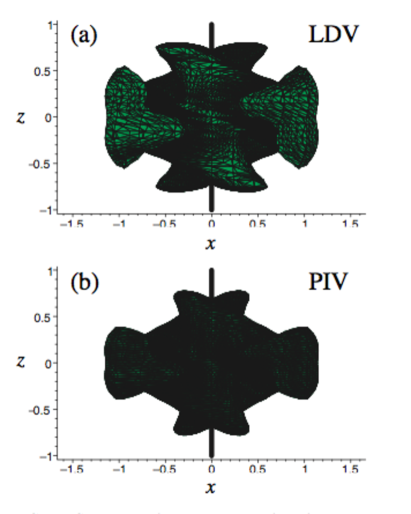
Figure 10: Comparison of the isodensity surface of magnetic energy ($50\%$ of the maximum) for LDV (a) and SPIV (b). The figures show the neutral mode close to onset $(R_{m}=44)$ with conducting layer $(w=0.6)$. A setup with (+) rotation and without annulus has been used. For SPIV the spline extrapolation with nrp=4 was used. The full line indicates the cylinder axis. Note, for $x>0$ (resp. $x<0$) the angle $\Theta$ is $0$ (resp. $\pi$).

In Fig. 10 we furthermore compare the isodensity surfaces of the magnetic energy of two runs for LDV and SPIV data with identical parameters. SPIV calculations have been done on a much finer grid in axial direction. Both facings look very similar, which is confirmed by quantitative measurements.

IV Kinematic dynamo simulations

IV.1 Results

Onset of dynamo action.— We have investigated the configurations in which the two propellers are exactly counter-rotating, in (+) and in (-) direction in setups with and without annulus. The computations have been made with nrp=2 to 6, and the critical Reynolds number is found by computing the growth rate for different magnetic reynolds numbers and the condition $\sigma(R_{m}^{c})=0$. The results are presented in Fig. 11 and 12 and summerized in Table 1.

In the presence of an annulus in the shear layer, the results show that the direction of rotation changes the critical magnetic Reynolds number by a factor 3 : $R_{m}^{c}\simeq 36$ for the (+) case and $R_{m}^{c}\simeq 113$ for the (-) case. There is an ever larger difference between the (+) and (-) rotation case when the annulus is absent: the dynamo threshold is $R_{m}^{c}\simeq 45$ for the (+) case, and $R_{m}^{c}>500$ in the (-) case.

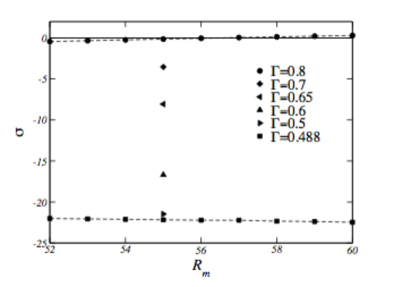
Figure 13: Influence of the poloidal to toroidal ratio $\Gamma$ on the magnetic growth rate $\sigma$. $\Gamma=0.488$ is the experimental value measured by SPIV in the experiment. The other cases correspond to artificial fields. A setup without annulus and (-) rotation has been used. For the spline extrapolation we fixed nrp=4.

These differences can be traced back to a difference in the poloidal to toroidal ratio $\Gamma$, that is much lower in the (-) case ($0.62$ with annulus and $0.49$ without annulus) than in the (+) case ($0.8$ with annulus or without annulus). This is in agreement with previous studies showing that the optimum for dynamo growth in von Karman type flows is around $\Gamma\approx 0.75$ RCD05 . Fig. 13 exhibits the influence of $\Gamma$ on the magnetic growth rate $\sigma$ in the (-) case without annulus: the growth rate of the synthetic fields increases very sharply with $\Gamma$ between $\Gamma=0.5$ and $\Gamma=0.8$.

The insertion of the annulus exhibits two effects: (i) in the (+) case, it decreases slighly ($15\%$) the critical magnetic Reynolds number while $\Gamma$ remains unchanged; (ii) in the (-) case, it increases the poloidal to toroidal ratio $\Gamma$ towards the range where dynamo action is available.

In the (+) case, both mean poloidal and toroidal flow increase when the annulus is inserted, but their ratio $\Gamma$ does not change within the error bars. However, with the annulus, the axial gradient of the toroidal flow is larger in the region of the shear layer (cf. Fig. 7): the gradient seems to be ”less spread out” by the coherent structures. In fact, the annulus has been intruduced in the VKS experiment to have an effect on the turbulent fluctuations, in particular on the large scale fluctuations, by stabilizing the shear layer vortices in the annulus plane. Indeed, the mean value of the normalized kinetic energy $\delta(t)$ decreases from $\bar{\delta}=2.02$ to $1.48$ and its variance $\delta_{2}$ decreases from $0.18$ to $0.12$ (cf. CDM09 ). This means that in the configuration with the annulus, the instantaneous flow is much closer to the mean flow. This quantity has not been measured in the Riga and Karlsruhe experiments, but one can suspect that the instantaneous flow is very close to the mean flow, which explains the very good agreement between kinematic dynamo simulations and experiments for these configurations. This is not the case for the VKS experiment, in which turbulent fluctuations are present at all scales. The annulus thus appears as a mean to reduce this problem, in particular for the large scales.

In the (-) case, $\Gamma$ has a low value without annulus, because both the toroidal part of the flow has increased and the poloidal part decreased. This low value is clearly out of the range for dynamo action in these flows. Moreover, the turbulent fluctuations are more intense in this sense of rotation and the corresponding values of $\bar{\delta}$ and $\delta_{2}$ are larger than in the (+) case. The insertion of the annulus has two effects. First, it increases the poloidal to toroidal ratio, opening the possibility to get dynamo action, but still at large $R_{m}^{c}$. Second, it reduces $\bar{\delta}$ from $2.22$ to $1.50$ and its variance $\delta_{2}$ from $0.24$ to $0.11$ (cf. CDM09 ), leading to values similar to the (+) case with annulus.

Magnetic growing mode.— The fastest growing mode we observe is always a $m=1$ mode. Recall that since our configuration and flow are axisymmetric by construction and there are no external field source, the generation of a $m=0$ mode is forbidden by Cowling’s theorem M78 . Sections of the magnetic field obtained in the different configurations are presented in Fig. 14 and Fig. 15. The configuration corresponding to (+) case without annulus is in agreement with the results of RCD05 . The magnetic field in the (+) case with annulus reveals a sharper field….XXXXXXXX

In the (-) case without annulus, the synthetic field with $\Gamma=0.8$ looks very similar to the (+) case. On the contrary, the (-) case with annulus, that corresponds to a larger $R_{m}^{c}$ is very different from the 3 other cases.. XXXXXXXXXXXX

IV.2 Comparison with experiments

Onset of dynamo action.— When comparing these kinematic simulations results with experimental one, one observes that if the exact values are note recovered, the order of magnitude of the dynamo threshold $R_{m}^{c}$ as well as the general trend are correctly reproduced: with annulus, $R_{m}^{c}$ is larger for the (-) case than for the (+) case, and there is no dynamo in the (-) case without annulus in the available experimental $R_{m}$ range.

The fact that the thresholds obtained in simulations are different from the experimental ones is not surprising: the simulations presented in this paper have been performed with real mean flows but in an over-simplified VKS configuration. First of all, the lateral boundary conditions (shell of sodium at rest) have been taken into account but not the end boundaries (sodium behind the disks). However, the effect is in general to increase $R_{m}^{c}$ (SXG06 ), whereas the experimental values are smaller than the numerical ones. Then, the effect of the soft-iron impellers (magnetic permeability $\sim 100$) has also been discarded. Using the synthetic MND flow MND06 to describe the von Karman mean axisymmetric flow, it has been shown that infinite permability boundary conditions are able to reduce the dynamo threshold by $5\%$ to $10\%$ GIFD08 . Finally, and perhaps more importantly, turbulence is not adressed in the simulations, whereas the Reynolds number of the VKS experiment is between $10^{6}$ and $10^{7}$ P5 . Only the mean axisymmetric flow is used in the simulations : the large scale vortices of the shear layer as well as the blades vortices are not considered, neither small scale turbulence. Non axisymmetric fluctuations, such as those generated by the flow ejected by the blades of the impellers, could e.g. generate an $\alpha$ effect and give rise to an alpha-omega type dynamo GAFDFauve . The addition in the induction equation of an empirical alpha term localized in the vicinity of the impellers displays an axial dipole but the value of $\alpha$ required to obtain the experimental threshold appears to be unrealistic LNRLGP08 .

Very recent kinematic simulations with synthetic flows have been reported in two directions. First, by adding a modelization of the non axisymmetric vortices ejected by the blades of the propellers to the synthetic MND mean axisymmetric flow, G09 has evidenced dynamo action with an axial dipole or quadrupole for $R_{m}^{c}\simeq 34$. Second, by adding a localized permeability distribution that mimics the shape of the impellers disk and blades, GSG09 has found an equatorial dipole for $R_{m}^{c}\simeq 60$ without $\alpha$ effect and an axial dipole for $R_{m}^{c}\simeq 32$ when including an $\alpha$ effect with a realistic value.

Magnetic growing mode.— In all the studied cases the structure of the kinematic neutral mode is a $m=1$ equatorial dipole mode. In the VKS experiment, the structure of the saturated has been reported in the (+) rotation sense, with annulus, and found to correspond mainly to a $m=0$ mode MBB07 ; P5 . It would be interesting to have detailed measurements of the saturated mode structure in the VKS experiment, for the different configurations and in particular in the reverse rotation direction. One can e.g. wonder whether or not a $m=1$ component is present besides the axial dipole.

As reported above, recent simulations have exhibited an axial dipole (or quadrupole) with synthetic flows and particular boundary conditions, and it would be of great interest to study the effect of the annulus and the direction of rotation on these results.

V Concluding remarks

Through kinematic simulations using SPIV velocity fields measured in a water model experiment, we have shown that the rotation direction of the non axisymmetric impellers in the VKS experiment has a great impact on the threshold of the dynamo generated by the mean flow only. By changing the rotation direction, one can increase the dynamo threshold by a factor 3 in the case with annulus (1.4 in the VKS experiment), and a factor larger than 10 in the case without annulus (larger than 1.6 in the VKS experiment). Even if the exact experimental results are not reproduced, the variation of the dynamo threshold with the direction sense is qualitatively reproduced by the kinematic simulations.

Since our kinematic simulations do not take into account the magnetic permeability due to iron disks-an effect that can decrease the threshold by a factor 2 (cf. GIFD08 ) or generate a m=0 mode with an $\alpha$ effect GSG09 , we do not expect our results to be more than qualitative. Furthermore, our linear simulations do not take into account the back reaction of the Lorentz force, that can enforce emergence of the m=0 mode as a secondary bifurcation of the original m=1 mode GDF08 . Finally, non axisymmetric turbulent fluctuations can play an important role in the generation of a magnetic dipole GAFDFauve ; G09 .

Nevertheless, we have shown that the increase (or the absence) of the dynamo threshold observed in given configurations of the VKS experiment can have two origins: (i) the poloidal to toroidal ratio $\Gamma$, a parameter previously identified as crucial for dynamo action RCD05 . (ii) the normalized kinetic energy $\delta$ which quantifies the distance of the instaneous flow to the mean flow. The parameter $\Gamma$ is certainly important for the alpha-omega mechanism proposed in GAFDFauve , giving the relative importance of the $\alpha$ effect generated by the blades vortices (poloidal recirculation) vs. the omega effect due to differential rotation (toroidal flow).

Detailed experimental study of the propellers vortices dynamics with the rotation direction would represent an important step to validate the numerical predictions. Work is in progress in this direction.

Rotation sense	annulus	$\Gamma$	$\bar{\delta}$	$\delta_{2}$	$R_{m}^{c}{\rm exp}$	$R_{m}^{c}{\rm sim}$
+	with	$0.8$	$1.48$	$0.12$	$\approx 32$	$35.6-37.7$
+	without	$0.8$	$2.02$	$0.18$	$\approx 32$	$41.6-47.6$
-	with	$0.62$	$1.50$	$0.11$	$\approx 43$	$\approx 113$
-	without	$0.49$	$2.22$	$0.24$	$>50$	$>500$
-	without	$0.8$	(*)	(*)	(*)	$\approx 57$

Table 1: Comparison of experimental and numerical critical magnetic Reynolds numbers for the different VKS setups. An interval for $R_{m}^{c}{sim}$ is given when different nrp have been used (cf. Fig. 9 and 11), otherwise nrp=4. (*) denotes an artificial numerical field with a prepared $\Gamma$ not available in experiments. The values of the mean normalized kinetic energy $\bar{\delta}$ and its variance $\delta_{2}$ are from CDM09

Figure 1: (a) Sketch of the simulated part of the VKS experiment (cross section) including both impellers (I1,I2) and an annulus (A) at mid height. The horizontal axis corresponds to the $z$ axis. The container radius $R$ is taken as length scale. The factor $w$ denotes the thickness of the conducting layer (grey area) of sodium at rest in the VKS experiment. The layers of sodium between the impellers and the end walls of cylinder have not been taken into account in this work. (b) Top view of the TM 73 impellers used in the VKS experiment RCD05 . The (+) (resp. (-)) rotation sense corresponds to a counterclockwise (resp. clockwise) rotating impeller.

Figure 2: Dimensionless velocity field measured by SPIV in VKE and symmetrized as well as spline extrapolated (nrp=4) for kinematic dynamo simulations (see text for details). (a) (+) rotation and no annulus (NA); (b) (+) rotation and presence of an annulus (WA); (c) (-) rotation and no annulus (NA); (d) (-) rotation and presence of an annulus (WA); The coloring displays the velocity field perpendicular to the plane, whereas red (blue) denotes a positive (negative) sign in cylindrical coordinates $(r,\Theta,z)$. The white area for radii $r>1$ shows the conducting layer at rest $(w=0.6)$ with $\mathbf{u}=0$.

Figure 6: Same as in Fig. 4 for a setup with (+) rotation and the presence of an annulus at mid height.

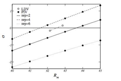
Figure 9: Magnetic energy growth rate $\sigma$ vs. $R_{m}$ for a setup with a conducting layer $(w=0.4)$ and a flow obtained with (+) rotation and without annulus, $\Gamma=0.8$. Full (open) symbols refer to SPIV (LDV) data. For SPIV the results for different spline fits are compared, cf. figures 4 and 5, respectively.

Figure 11: Same as in Fig. 9 for a setup with (+) rotation and the presence of an annulus at mid height, $\Gamma=0.8$.

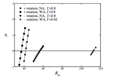
Figure 12: Magnetic energy growth rate $\sigma$ vs. $R_{m}$ for different setups with conducting layer $(w=0.4)$. WA (resp. NA) denotes configurations with (resp. without) annulus. For all cases nrp=4 has been used. Note that the case (-) rotation without annulus corresponds to an artificial numerical field with $\Gamma=0.8$ not available in experiments.

Figure 14: Sections of the magnetic field $\mathbf{b}$ for different experimental setups, here for fixed $\Theta=0$. All configurations are with conducting layer $(w=0.4)$, whereas WA (resp. NA) specifies setups with (resp. without) annulus. Arrows correspond to components lying in the cut plane and the color code to the component transverse to the cut plane, where red (resp. blue) denotes a positive (resp. negative) sign. Parameters are (a) $R_{m}=44$, $\Gamma=0.8$, (b) $R_{m}=40$, $\Gamma=0.8$, (c) $R_{m}=60$, $\Gamma=0.8$ (artificial field), (d) $R_{m}=115$, $\Gamma=0.62$. For all cases nrp=4 has been used.

Figure 15: Same as in Fig. 11, for $\Theta=\pi/2$.

References

- (1) J. Larmor, Rep. Brit. Assoc. Adv. Sci., pp. 159-160 (1919)
- (2) A. Gailitis et al., Phys. Rev. Lett. 86, 3024 (2001).
- (3) R. Stieglitz and U. Müller, Phys. Fluids 13, 561 (2001).
- (4) Yu. B. Ponomarenko, J. Appl. Mech. Tech. Phys. 14, 775-778 (1973)
- (5) G.O. Roberts, Phil. Trans. Roy. Soc. London A 271, 411-454 (1972)
- (6) R. Monchaux, M. Berhanu, M. Bourgoin, M. Moulin, Ph. Odier, J.-F. Pinton, R. Volk, S. Fauve, N. Mordant, F. Pétrélis, A. Chiffaudel, F. Daviaud, B. Dubrulle, C. Gasquet, L. Marié, and F. Ravelet, Phys. Rev. Lett. 98, 044502 (2007).
- (7) M. Berhanu, R. Monchaux, S. Fauve, N. Mordant, F. Pétrélis, A. Chiffaudel, F. Daviaud, B. Dubrulle, L. Marié, F. Ravelet, M. Bourgoin, Ph. Odier, J.-F. Pinton, and R. Volk, Europhys. Lett. 77, 59001 (2007).
- (8) F. Ravelet, M. Berhanu, ,R. Monchaux, S. Aumaitre, A. Chiffaudel, F. Daviaud, B. Dubrulle, M. Bourgoin, Ph. Odier, J.-F. Pinton, N. Plihon, R. Volk, S. Fauve, N. Mordant and F. Pétrélis, Phys. Rev. Lett. 101, 074502(2008).
- (9) R. Monchaux, M. Berhanu, S. Aumaitre, A. Chiffaudel, F. Daviaud, B. Dubrulle, F. Ravelet, S. Fauve, N. Mordant, F. Pétrélis, M. Bourgoin, Ph. Odier, J.-F. Pinton, N. Plihon and R. Volk, Phys. Fluids 21, 035108 (2009).
- (10) F. Ravelet, A. Chiffaudel and F. Daviaud, J. Fluid Mech. 601, 339-364 (2008)
- (11) P.-P. Cortet, P. Diribarne, R. Monchaux, A. Chiffaudel, F. Daviaud and B. Dubrulle. Phys. Fluids 21, 025104 (2009).
- (12) L. Marié, C. Normand, and F. Daviaud, Phys. Fluids 18, 1 (2006).
- (13) L. Marié, J. Burguete, F. Daviaud, and J. Léorat, Eur. Phys. J. B 33, 469 (2003).
- (14) F. Ravelet, A. Chiffaudel, F. Daviaud and J. Léorat, Phys. Fluids 17, 117104 (2005)
- (15) F. Pétrélis, N. Mordant and S. Fauve, Geophys. Astrophys. fluid Dyn. 101, 289 (2007).
- (16) R. Laguerre, C. Nore, A. Ribeiro, J. Léorat, J-L. Guermond and F. Plunian Phys. Rev. Lett. 101, 104501 (2008).
- (17) C. Gissinger, E. Dormy and S. Fauve Phys. Rev. Lett. 101, 144502 (2008).
- (18) R. Avalos-Zuniga, F. Plunian and A. Gailitis Phys. Rev. E68, 066307 (2003).
- (19) C. Gissinger, A. Iskakov, S. Fauve and E. Dormy Europhys. Lett. 82, 29001 (2008).
- (20) F. Stefani, M. Xu, G. Gerbeth, F. Ravelet, A. Chiffaudel, F. Daviaud and J. Léorat, Eur. J. Mech. B25, 894 (2006)
- (21) P. Livermore and A. Jackson, Proc. Roy. Soc. A 462, 2457 (2006).
- (22) Y. Ponty, J.-P. Laval, B. Dubrulle, F. Daviaud, and J.-F. Pinton, Phys. Rev. Lett. 99, 224501 (2007).
- (23) Forest
- (24) Lathrop
- (25) Y. Ponty, P. D. Minnini, D. Montgomery, J.-F. Pinton, H. Politano and A. Pouquet, Phys. Rev. Lett. 94, 164502 (2005).
- (26) J.-P. Laval, P. Blaineau, N. Leprovost, B. Dubrulle, and F. Daviaud, Phys. Rev. Lett. 96, 204503 (2006).
- (27) B. Dubrulle, P. Blaineau, O. Mafra-Lopez, F. Daviaud, J.-P. Laval and R. Dolganov, New J. Phys. 9, 308 (2007).
- (28) R. Monchaux, Mécanique statistique et effet dynamo dans un écoulement de von Kármán turbulent, PhD thesis, Université de Paris 7 (2007).
- (29) F. Ravelet, L. Marié, A. Chiffaudel, F. Daviaud, Phys. Rev. Lett. 93, 164501 (2004).
- (30) J. Léorat, Numerical simulations of cylindrical dynamos: Scope and method, in Progress in Turbulence Research, Progress in Astronautics and Aeronautics, Vol. 162 (AIAA, Washington,1994),p. 282.
- (31) H.K. Moffatt, Magnetic field generation in electrically conducting fluids, Cambridge University Press, Cambridge, 1978
- (32) C. Gissinger, A numerical model of the VKS experiment, ArXiv:0906.3792 (2009)
- (33) A. Giesecke, F. stefani and G. Gerbeth, Role of soft-iron impellers on the mode selection in the VKS dynamo experiment, preprint (2009)