Correlation induced switching of local spatial charge distribution in two-level system

Abstract

We present theoretical investigation of spatial charge distribution in the two-level system with strong Coulomb correlations by means of Heisenberg equations analysis for localized states total electron filling numbers taking into account pair correlations of local electron density. It was found that tunneling current through nanometer scale structure with strongly coupled localized states causes Coulomb correlations induced spatial redistribution of localized charges. Conditions for inverse occupation of two-level system in particular range of applied bias caused by Coulomb correlations have been revealed. We also discuss possibility of charge manipulation in the proposed system.

I Introduction

Investigation of tunneling properties of interacting impurity complexes in the presence of Coulomb correlations is one of the most important problems in the physics of nanostructures. Tunneling current changes localized states electron filling numbers as a result-the spectrum and electron density of states are also modified due to Coulomb interaction of localized electrons. Moreover the charge distribution in the vicinity of such complexes can be tuned by changing the parameters of the tunneling contact. Self-consistent approach based on Keldysh diagram technique have been successfully used to analyze non-equilibrium effects and tunneling current spectra in the system of two weakly coupled impurities (when coupling between impurities is smaller than tunneling rates between energy levels and tunneling contact leads) in the presence of Coulomb interaction Keldysh . In the mean-field approximation for mixed valence regime the dependence of electron filling numbers on applied bias voltage and the behaviour of tunneling current spectra have been analyzed in Arseyev .

Electron transport even through a single impurity in the Coulomb blockade and the Kondo regime Kondo have been studied experimentally and is up till now under theoretical investigation Goldin -Kikoin . As tunneling coupling is not negligable the impurity charge is not the discrete value and one has to deal with impurity electron filling numbers (which now are continuous variables) determined from kinetic equations.

Analyzing non-equilibrium tunneling processes through coupled impurities one can reveal switching on and off of magnetic regime (electron filling numbers in the localized states for opposite spins are equal) on each impurity atom at particular range of applied bias voltage Arseyev .

In the present work we consider the opposite case when coupling between localized electron states strongly exceeds tunneling transfer rates. This situation can be experimentally realized when several impurity atoms or surface defects are situated at the neighboring lattice sites, so coupling between their electronic states can strongly exceeds the interaction of this localized states with continuous spectrum Fig.1. Another possible realization is two interacting quantum dots on the sample surface weakly connected with the bulk states. Such systems can be described by the model including several electron levels with Coulomb interaction between localized electrons. If the distance between impurities is smaller than localization radius, strong enough correlation effects arise which modify the spectrum of the whole complex. Electronic structure of such complexes can be tuned as by external electric field which changes the values of single particle levels as by electron correlations of localized electronic states. One can expect that tunneling current induces non-equilibrium spatial redistribution of localized charges and gives possibility of local charge density manipulation strongly influenced by Coulomb correlations. In some sense these effects are similar to the $"$co-tunneling$"$ observed in Feigel'man , Beloborodov . Moreover Coulomb interaction of localized electrons can be responsible for inverse occupation of localized electron states. These effects can be clearly seen when single electron levels have different spatial symmetry.

To understand such correlation induced $"$charge$"$ switching it’s sufficient to analyze Heisenberg equations for localized states total electron filling numbers taking into account pair correlations of local electron density Maslova . If one is interested in kinetic properties and changes of local charge density for the applied bias range higher than the value of energy levels tunneling broadening modification of initial density of states due to the Kondo effect can be neglected. In this case for the finite number of localized electron levels one can obtain closed system of equations for electron filling numbers and their higher order correlations.

II The suggested model

We shall analyze tunneling through the two-level system with Coulomb interaction Fig.1. The model system can be described by the Hamiltonian $\hat{H}$.

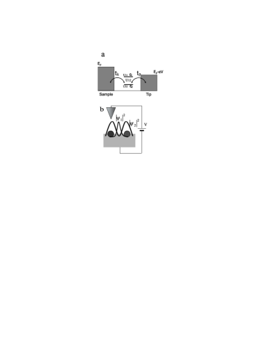
Figure 1: a). Energy diagram of two-level system and b). Schematic spatial diagram of experimental realization. Coulomb energy $U_{12}$ correspond to the interaction between electrons on different energy levels.

$$\hat{H} = \sum_{i\sigma}\varepsilon_{i}n_{i\sigma}+\sum_{k\sigma}\varepsilon_{k}c_{k\sigma}^{+}c_{k\sigma}+\sum_{p\sigma}\varepsilon_{p}c_{p\sigma}^{+}c_{p\sigma}+$$ (1)

$$+ \sum_{ij\sigma\sigma^{{}^{\prime}}}U_{ij}^{\sigma\sigma^{{}^{\prime}}}n_{i\sigma}n_{j\sigma^{{}^{\prime}}}+\sum_{ki\sigma}t_{k}c_{k\sigma}^{+}c_{i\sigma}+$$

$$+ \sum_{pi\sigma}t_{p}c_{p\sigma}^{+}c_{i\sigma}+h.c.\$$

Indices $k$ and $p$ label continuous spectrum states in the left (sample) and right (tip) leads of tunneling contact respectively. $t_{k(p)}$- tunneling transfer amplitudes between continuous spectrum states and two-level system with elctron levels $\varepsilon_{i}$. Operators $c_{k(p)}^{+}/c_{k(p)}$ correspond to electrons creation/annihilation in the continuous spectrum states $k(p)$. $n_{i\sigma}=c_{i\sigma}^{+}c_{i\sigma}$-two-level system electron filling numbers, where operator $c_{i\sigma}$ destroys electron with spin $\sigma$ on the energy level $\varepsilon_{i}$. $U_{ij}^{\sigma\sigma^{{}^{\prime}}}$ is the on-site Coulomb repulsion of localized electrons.

Tunneling current through the two-level system can be written in the terms of electron creation/annihilation operators as:

$$I=I_{k\sigma}=\sum_{k\sigma}\dot{n}_{k\sigma}=\sum_{ki\sigma}t_{k}(<c_{k\sigma}^{+}c_{i\sigma}>-<c_{i\sigma}^{+}c_{k\sigma}>)$$ (2)

Let us consider $\hbar=1$ elsewhere, so motion equation for the electron operators product $c_{k\sigma}^{+}c_{i\sigma}$ can be written as:

$$i\frac{\partial c_{k\sigma}^{+}c_{i\sigma}}{\partial t} = (\varepsilon_{i}-\varepsilon_{k})\cdot c_{k\sigma}^{+}c_{i\sigma}+U_{ii}n_{i-\sigma}\cdot c_{k\sigma}^{+}c_{i\sigma}+$$ (3)

$$+ U_{ij}(n_{j\sigma}+n_{j-\sigma})\cdot c_{k\sigma}^{+}c_{i\sigma}-t_{k}\cdot(n_{i\sigma}-\widehat{f}_{k})+$$

$$+ \sum_{k^{{}^{\prime}}\neq k}t_{k^{{}^{\prime}}}c_{k\sigma}^{+}c_{k^{{}^{\prime}}\sigma}+\sum_{i\neq j}t_{k}c_{j\sigma}^{+}c_{i\sigma}=0$$

where

$$\widehat{f}_{k}=c_{k\sigma}^{+}c_{k\sigma}$$ (4)

Now let us also consider that $n_{i\sigma}^{2}=n_{i\sigma}$.

Neglecting changes of electron spectrum and local density of states in the tunneling contact leads due to the tunneling current flowing we shall uncouple conduction and two-level system electron filling numbers. After summation over $k$ one can get an equation which describe tunneling current in the presented two-level system:

$$I_{k\sigma}=I_{k1\sigma}+I_{k2\sigma}$$ (5)

Where expression for tunneling current $I_{k2\sigma}$ can be obtained by changing indexes $1\leftrightarrow 2$ in equation for tunneling current $I_{k1\sigma}$ which has the form:

$$I_{k1\sigma} = \Gamma_{k}\cdot\{\langle n_{1\sigma}\rangle+\sum_{j\neq i}\langle c_{j\sigma}^{+}c_{i\sigma}\rangle-$$

$$- \langle(1-n_{1-\sigma})(1-n_{2-\sigma})(1-n_{2\sigma})\rangle\cdot f_{k}(\varepsilon_{1})-$$

$$- \langle n_{1-\sigma}(1-n_{2-\sigma})(1-n_{2\sigma})\rangle\cdot f_{k}(\varepsilon_{1}+U_{11})-$$

$$- \sum_{\sigma^{{}^{\prime}}}\langle n_{2\sigma^{{}^{\prime}}}(1-n_{2-\sigma^{{}^{\prime}}})(1-n_{1-\sigma})\rangle\cdot f_{k}(\varepsilon_{1}+U_{12})-$$

$$- \sum_{\sigma^{{}^{\prime}}}\langle n_{1-\sigma}n_{2\sigma^{{}^{\prime}}}(1-n_{2-\sigma^{{}^{\prime}}})\rangle\cdot f_{k}(\varepsilon_{1}+U_{11}+U_{12})-$$

$$- \langle n_{2\sigma}n_{2-\sigma}(1-n_{1-\sigma})\rangle\cdot f_{k}(\varepsilon_{1}+2U_{12})-$$

$$- \langle n_{1-\sigma}n_{2-\sigma}n_{2\sigma}\rangle\cdot f_{k}(\varepsilon_{1}+U_{11}+2U_{12})\}+$$

$$+ \sum_{k^{{}^{\prime}}\neq k}\langle t_{k}t_{k^{{}^{\prime}}}c_{k\sigma}^{+}c_{k^{{}^{\prime}}\sigma}\rangle\cdot$$

$$\cdot \{\langle\frac{(1-n_{1-\sigma})(1-n_{2-\sigma})(1-n_{2\sigma})}{\varepsilon_{1}-\varepsilon_{k}}\rangle+$$

$$+ \langle\frac{n_{1-\sigma}(1-n_{2-\sigma})(1-n_{2\sigma})}{\varepsilon_{1}+U_{11}-\varepsilon_{k}}\rangle+$$

$$+ \langle\frac{\sum_{\sigma^{{}^{\prime}}}n_{2\sigma^{{}^{\prime}}}(1-n_{1-\sigma})(1-n_{2-\sigma^{{}^{\prime}}})}{\varepsilon_{1}+U_{12}-\varepsilon_{k}}\rangle+$$

$$+ \langle\frac{\sum_{\sigma^{{}^{\prime}}}n_{1-\sigma}n_{2\sigma^{{}^{\prime}}}(1-n_{2-\sigma^{{}^{\prime}}})}{\varepsilon_{1}+U_{11}+U_{12}-\varepsilon_{k}}\rangle+$$

$$+ \langle\frac{n_{2-\sigma}n_{2\sigma}(1-n_{1-\sigma})}{\varepsilon_{1}+2U_{12}-\varepsilon_{k}}\rangle+\langle\frac{n_{1-\sigma}n_{2-\sigma}n_{2\sigma}}{\varepsilon_{1}+U_{11}+2U_{12}-\varepsilon_{k}}\rangle\}$$

We shall further neglect terms $t_{k}c_{i\sigma}^{+}c_{j\sigma}$ and $t_{k}c_{k\sigma}^{+}c_{k^{{}^{\prime}}\sigma}$ in expression LABEL:current as they correspond to the next order perturbation theory by the parameter $\frac{\Gamma_{i}}{\Delta\varepsilon_{i}}$. Relaxation rates $\Gamma_{k(p)}=\pi\cdot t_{k(p)}^{2}\cdot\nu_{0}$ are determined by electron tunneling transitions from two-level system to the leads $k$ (sample) and $p$ (tip) continuum states. $\nu_{0}$-continuous spectrum density of states. Equations for filling numbers $n_{1\sigma}$ $n_{2\sigma}$ can be found from the conditions:

$$\frac{\partial n_{1\sigma}}{\partial t}=I_{k1\sigma}+I_{p1\sigma}=0$$

$$\frac{\partial n_{2\sigma}}{\partial t}=I_{k2\sigma}+I_{p2\sigma}=0\$$ (7)

where tunneling current $I_{p\sigma}$ can be easily determined from $I_{k\sigma}$ by changing indexes $k\leftrightarrow p$

We shall analyze the situation when Coulomb energy values are large and condition $U_{ij}>>\varepsilon_{i/j}$ can be taken into account. It means that if one have to calculate tunneling current through such system it is necessary to find all pair filling numbers correlators in the energy range $\varepsilon_{i}+U_{ij}$. So we retain the terms containing $f_{k(p)}(\varepsilon_{i}+U_{ij})$ and neglect all high orders correlators and pair correlators which contain $f_{k(p)}(\varepsilon_{i}+U_{ij}+U_{kl})$. We consider the paramagnetic situation $n_{i\sigma}=n_{i-\sigma}$.

Pair filling numbers correlators can be found in the following way:

$$\langle\frac{\partial n_{i\sigma}n_{j\sigma^{{}^{\prime}}}}{\partial t}\rangle=\langle\frac{\partial n_{i\sigma}}{\partial t}n_{j\sigma^{{}^{\prime}}}\rangle+\langle\frac{\partial n_{j\sigma^{{}^{\prime}}}}{\partial t}n_{i\sigma}\rangle$$ (8)

Let us introduce tunneling filling numbers $n^{T}(\varepsilon_{i})$, $n^{T}(\varepsilon_{i}+U_{ij})$ and $\tilde{n}_{ij}^{T}$ which have the form:

$$n^{T}(\varepsilon_{i}) = \frac{\Gamma_{k}f_{k}(\varepsilon_{i})+\Gamma_{p}f_{p}(\varepsilon_{i})}{\Gamma_{k}+\Gamma_{p}}$$

$$n^{T}(\varepsilon_{i}+U_{ij}) = \frac{\Gamma_{k}f_{k}(\varepsilon_{i}+U_{ij})+\Gamma_{p}f_{p}(\varepsilon_{i}+U_{ij})}{\Gamma_{k}+\Gamma_{p}}$$

$$\tilde{n}_{ij}^{T} = \frac{\Gamma_{k}\tilde{f}_{kij}+\Gamma_{p}\tilde{f}_{pij}}{\Gamma_{k}+\Gamma_{p}}$$ (9)

where

$$\tilde{f}_{kij}=f_{k}(\varepsilon_{i})-f_{k}(\varepsilon_{i}+U_{ij})\$$ (10)

As we consider that $n_{i\sigma}=n_{i-\sigma}$, let us also consider $\langle n_{i\sigma}n_{j\sigma}\rangle=\langle n_{i\sigma}n_{j-\sigma}\rangle$. So a system of equations for pair correlators $K_{11}\equiv\langle n_{1\sigma}n_{1-\sigma}\rangle$, $K_{22}\equiv\langle n_{2\sigma}n_{2-\sigma}\rangle$ and $K_{12}\equiv\langle n_{1\sigma}n_{2\sigma}\rangle$ for large Coulomb energies $U_{ij}>>\varepsilon_{i/j}$ has the form:

$$\begin{pmatrix}a_{11}&&a_{12}&&a_{13}\\ a_{21}&&a_{22}&&a_{23}\\ a_{31}&&a_{32}&&a_{33}\end{pmatrix}\times\begin{pmatrix}K_{11}\\ K_{22}\\ K_{12}\end{pmatrix}=F$$ (11)

where

$$a_{11} = a_{23}=1$$

$$a_{13} = a_{21}=0$$

$$a_{12} = 2n^{T}(\varepsilon_{1}+U_{11})$$

$$a_{22} = 2n^{T}(\varepsilon_{2}+U_{22})\$$ (12)

$$a_{31} = \frac{1}{2}n^{T}(\varepsilon_{2}+U_{12})$$

$$a_{32} = 1+\frac{1}{2}n^{T}(\varepsilon_{1}+U_{12})+\frac{1}{2}n^{T}(\varepsilon_{2}+U_{12})$$

$$a_{33} = \frac{1}{2}n^{T}(\varepsilon_{1}+U_{12})\$$ (13)

and

$$F=\begin{pmatrix}n^{T}(\varepsilon_{1}+U_{11})\cdot n_{1\sigma}\\ n^{T}(\varepsilon_{2}+U_{22})\cdot n_{2\sigma}\\ \frac{1}{2}n^{T}(\varepsilon_{1}+U_{12})\cdot n_{2\sigma}+\frac{1}{2}n^{T}(\varepsilon_{2}+U_{12})\cdot n_{1\sigma}\\ \end{pmatrix}$$ (14)

Equations which determine two-level system filling numbers immediately follows from the system 11:

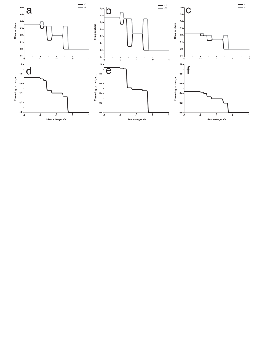
Figure 2: Two-level system filling numbers a).-c). and tunneling current d).-f). as a function of applied bias voltage in the case when both energy levels are situated above the sample Fermi level. Parameters $\epsilon_{1}=0.6$, $\epsilon_{2}=0.3$, $U_{12}=1.0$, $U_{11}=1.4$, $U_{22}=1.5$ are the same for all the figures. a),d).$\Gamma_{k}=0.01$, $\Gamma_{p}=0.01$; b),e).$\Gamma_{k}=0.05$, $\Gamma_{p}=0.01$; c),f).$\Gamma_{k}=0.01$, $\Gamma_{p}=0.03$.

$$n_{1\sigma} \cdot (1+\tilde{n}_{11}^{T})+n_{2\sigma}\cdot 2\tilde{n}_{12}^{T}-K_{22}\cdot(n^{T}(\varepsilon_{1})-2n^{T}(\varepsilon_{1}+U_{12}))+$$

$$+ 2\cdot K_{12}\cdot(-n^{T}(\varepsilon_{1})+n^{T}(\varepsilon_{1}+U_{11})+n_{T}(\varepsilon_{1}+U_{12}))=$$

$$= n^{T}(\varepsilon_{1})$$

$$n_{2\sigma} \cdot (1+\tilde{n}_{22}^{T})+n_{1\sigma}\cdot 2\tilde{n}_{21}^{T}-K_{11}\cdot(n^{T}(\varepsilon_{2})-2n^{T}(\varepsilon_{2}+U_{12}))+$$ (15)

$$+ 2\cdot K_{12}\cdot(-n^{T}(\varepsilon_{2})+n^{T}(\varepsilon_{2}+U_{22})+n_{T}(\varepsilon_{2}+U_{12}))=$$

$$= n^{T}(\varepsilon_{2})$$

And finally expression for tunneling current has the form:

$$I_{k1\sigma} = \Gamma_{k}\cdot\{\langle n_{1\sigma}\rangle-(1-\langle n_{1\sigma}\rangle-2\langle n_{2\sigma}\rangle+K_{22}+2K_{12})\cdot$$ (16)

$$\cdot f_{k}(\varepsilon_{1})-(\langle n_{1\sigma}\rangle-2K_{12})\cdot f_{k}(\varepsilon_{1}+U_{11})-$$

$$- 2\cdot(\langle n_{2\sigma}\rangle-K_{12}-K_{22})\cdot f_{k}(\varepsilon_{1}+U_{12})\$$

Let us also mention two extreme cases. The first one when all Coulomb energies are extremely large $U_{ij}\rightarrow\infty$. In this situation expressions for filling numbers will have the following form:

$$n_{1\sigma}=\frac{n^{T}(\varepsilon_{1})\cdot(1-n^{T}(\varepsilon_{2}))}{(1+n^{T}(\varepsilon_{1}))\cdot(1+n^{T}(\varepsilon_{2}))-4\cdot n^{T}(\varepsilon_{1})\cdot n^{T}(\varepsilon_{2})}$$

$$n_{2\sigma}=\frac{n^{T}(\varepsilon_{2})\cdot(1-n^{T}(\varepsilon_{1}))}{(1+n^{T}(\varepsilon_{1}))\cdot(1+n^{T}(\varepsilon_{2}))-4\cdot n^{T}(\varepsilon_{1})\cdot n^{T}(\varepsilon_{2})}$$

And the second one is when energy levels are generated, for example due to the orbital quantum number $\varepsilon_{1}=\varepsilon_{2}=\varepsilon$ and consequently $U_{ij}=U$. In this case filling numbers have the form:

$$n_{\sigma}=\frac{n^{T}(\varepsilon)}{1+3\cdot n^{T}(\varepsilon)}$$ (18)

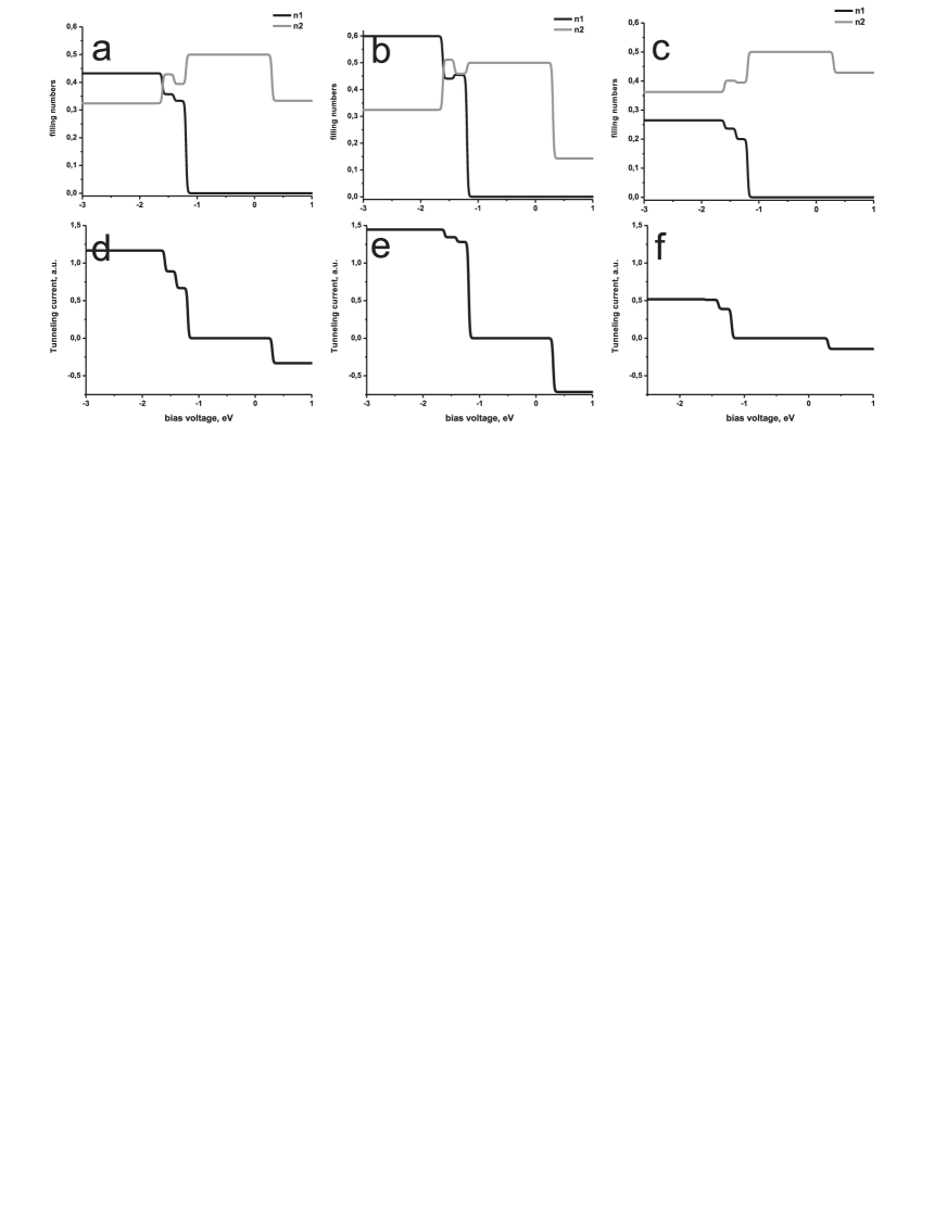
Figure 3: Two-level system filling numbers a).-c). and tunneling current d).-f). as a function of applied bias voltage in the case when one energy level is situated above and another one below the sample Fermi level. Parameters $\epsilon_{1}=0.2$, $\epsilon_{2}=-0.3$, $U_{12}=1.0$, $U_{11}=1.4$, $U_{22}=1.7$ are the same for all the figures. a),d).$\Gamma_{k}=0.01$, $\Gamma_{p}=0.01$; b),e).$\Gamma_{k}=0.05$, $\Gamma_{p}=0.01$; c),f).$\Gamma_{k}=0.01$, $\Gamma_{p}=0.03$.

III Main results and discussion

The behaviour of non-equilibrium electron filling numbers with changing of applied bias and tunneling conductivity characteristics obtained from equations (LABEL:current) and (11)-(16) are depicted on Fig.2-Fig.4.

We consider different experimental realizations: both energy levels are situated above the sample Fermi level (Fig.2); both levels below sample Fermi level (Fig.4) and one of the energy levels is located above the Fermi level and another one below the Fermi level (Fig.3). From the obtained results one can clearly see charge redistribution between two electron states with changing of applied bias voltage (Fig.2-4).

When both levels are situated above (Fig.2) or below (Fig.4) the sample Fermi level one can clearly reveal two possibilities for charge distribution in the two-level system. The first one corresponds to the case when local charge is mostly accumulated on the lower electron level $n_{1}<n_{2}$ ($\varepsilon_{2}<eV<\varepsilon_{1}$, $\varepsilon_{2}+U_{12}<eV<\varepsilon_{1}+U_{12}$ and $\varepsilon_{2}+U_{22}<eV<\varepsilon_{1}+U_{11}$ on Fig.2 and Fig.4). The second one deals with the case when charge is localized on both levels equally $n_{1}=n_{2}$ ($\varepsilon_{1}<eV<\varepsilon_{2}+U_{12}$, $\varepsilon_{1}+U_{12}<eV<\varepsilon_{2}+U_{22}$ and $\varepsilon_{1}+U_{11}<eV$ on Fig.2 and Fig.4).

Coulomb correlation induced sudden jumps down and up of each level electron filling numbers at certain values of applied bias are clearly seen.

So if electron states have essentially different symmetry one can expect charge accumulation in various spatial areas and thus the possibility of local charge manipulation appears.

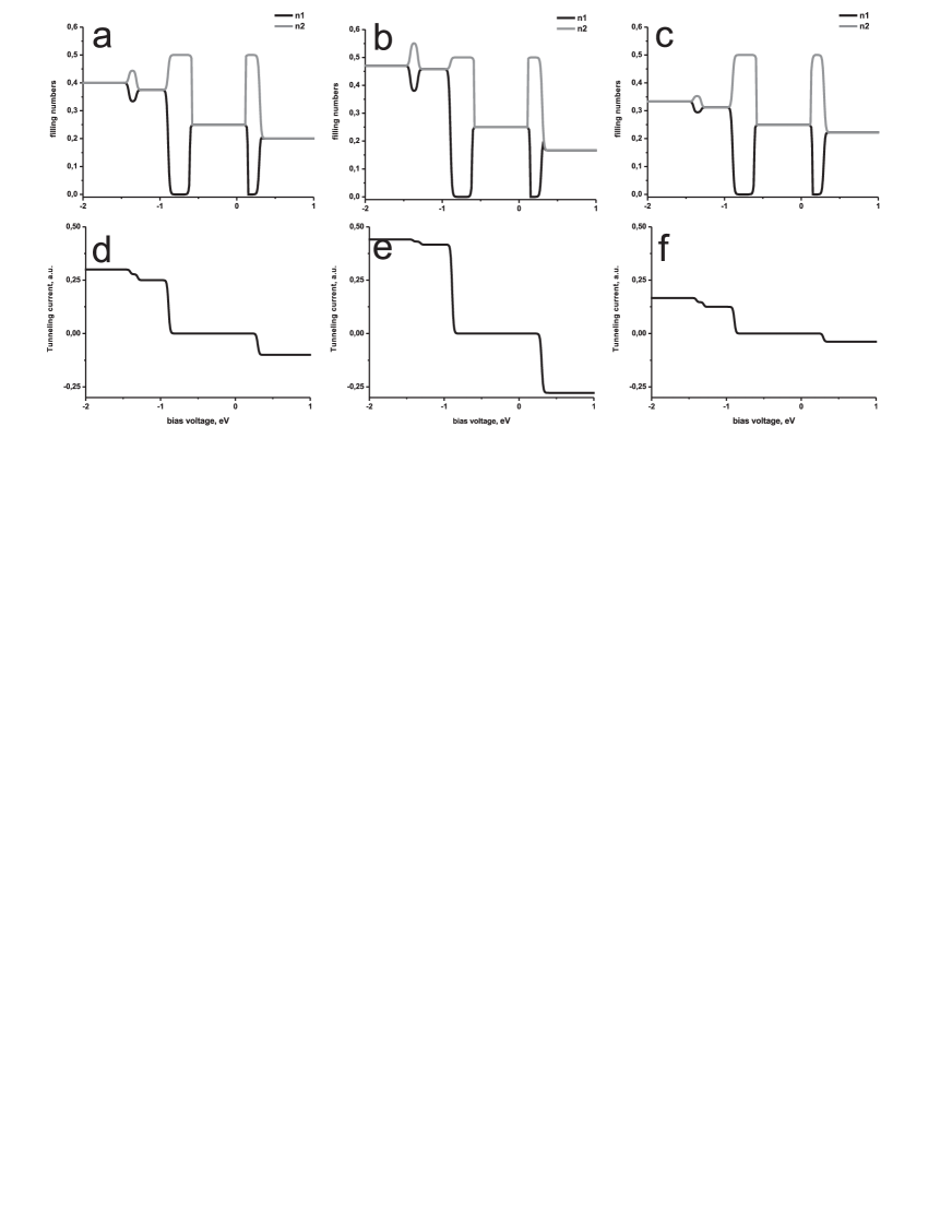
Figure 4: Two-level system filling numbers a).-c). and tunneling current d).-f). as a function of applied bias voltage in the case when both energy levels are situated below the sample Fermi level. Parameters $\epsilon_{1}=-0.1$, $\epsilon_{2}=-0.3$, $U_{12}=1.0$, $U_{11}=1.5$, $U_{22}=1.6$ are the same for all the figures. a),d).$\Gamma_{k}=0.01$, $\Gamma_{p}=0.01$; b),e).$\Gamma_{k}=0.05$, $\Gamma_{p}=0.01$; c),f).$\Gamma_{k}=0.01$, $\Gamma_{p}=0.03$.

When both electron energies are situated below the sample Fermi level upper electron state become empty ($n_{1}=0$) for two ranges of applied bias voltage ($\varepsilon_{2}<eV<\varepsilon_{1}$ and $\varepsilon_{2}+U_{12}<eV<\varepsilon_{1}+U_{12}$ )(Fig.4).

Described peculiarities take place for all the ratios between tunneling transfer rates $\Gamma_{k}$ and $\Gamma_{p}$.

The other interesting effect is the possibility of inverse occupation of the two-level system due to Coulomb interaction in special range of applied bias (Fig.3). In the absence of Coulomb interaction difference of electron filling numbers is determined by electron tunneling rates $n_{1}-n_{2}\sim\gamma_{k1}\gamma_{p2}-\gamma_{p1}\gamma_{k2}$. So without Coulomb interaction, for $\gamma_{k(p)1}=\gamma_{k(p)2}$, difference of the two levels occupation numbers turns to zero. Coulomb interaction of localized electrons in the two-level system results in inverse occupation of two levels at the high range of applied bias voltage. This situation is clearly demonstrated on the Fig.3.

It is clearly evident (Fig.3) that when applied bias doesn’t exceed value $\varepsilon_{1}+U_{12}$ all the charge is localized on the lower energy level ($n_{1}=0$). With the increasing of applied bias inverse occupation takes place and charge localized in the system redistributes. Local charge is mostly accumulated on the upper level when applied bias value exceed $\varepsilon_{1}+U_{11}$. Two-level system demonstrates such behaviour if the tunneling contact is symmetrical (Fig.3a) or when system strongly coupled with tunneling contact lead k (sample) (Fig.3b). We have not found inverse occupation when two-level system mostly coupled with tunneling contact lead p (tip) (Fig.3c). In this case with the increasing of applied bias upper electron state charge also increases but local charge continue being mostly accumulated on the lower electron state.

We also analyzed tunneling current as a function of applied bias voltage for different level’s positions (Fig.2-Fig.4d-f) . Tunneling current amplitudes presented in this work are normalized on $2\Gamma_{k}$ elsewhere. For all the values of the system parameters tunneling current dependence on applied bias has step structure. Height and length of the steps depend on the parameters of the tunneling contact (tunneling transfer rates and values of Coulomb energies). When both energy levels are above the Fermi level one can find six steps in tunneling current (Fig.2d-f). If both levels are situated below the Fermi level there are four steps in tunneling current (Fig.4d-f) and the upper electron level doesn’t appear as a step in current-voltage characteristics but charge redistribution takes place due to Coulomb correlations. One can also reveal four steps in the case when only lower energy level is situated below the Fermi level (Fig.3d-f).

IV Conclusion

Tunneling through the two-level system with strong coupling between localized electron states was analyzed by means of Heisenberg equations for localized states total electron filling numbers taking into account high order correlations of local electron density. Various electron levels location relative to the sample Fermi level in symmetric and asymmetric tunneling contact were investigated.

We revealed that charge redistribution between electron states takes place in suggested model when both electron levels are situated above or below the sample Fermi level. Charge redistribution is governed by Coulomb correlations. Moreover with variation of Coulomb interaction of localized electrons one can find the bias range of the two-level system inverse occupation when electron levels are localized on the opposite sites of the sample Fermi level.

This work was partially supported by RFBR grants.

References

• (1) L.V. Keldysh, Sov. Phys. JETP 20 ,1018 (1964)
• (2) P.I. Arseyev, N.S. Maslova, V.I. Panov, S.V. Savinov,JETP 121 ,225 (2002)
• (3) J. Kondo, Prog. Theor. Phys. 32 ,37 (1964)
• (4) Y. Goldin, Y. Avishai, Phys.Rev B 61,16750 (2000)
• (5) A.-P. Jauho, N.S. Wingreen, Y.Meir, Phys.Rev B 50,5528 (1994)
• (6) J. Konig, T. Pohjola, H.Schoeller, G. Schon, Physica E 6,371 (2000)
• (7) Y. Meir, N.S. Wingreen, P.A. Lee, Phys.Rev.Lett. 66,3048 (1991)
• (8) D.V. Averin, A.N. Korotkov, K.K. Likharev, Phys.Rev B 44,6191 (1991)
• (9) I.M. Ruzin, V. Chandrasekhar, E. Levin, L. Glazman, Phys.Rev B 45,13469 (1992)
• (10) K. Kikoin, Y. Avishai, Phys.Rev Lett. 86,2090 (2001)
• (11) M.V. Feigel’man, A.S. Ioselevich, JETP Letters 81 ,341 (2005)
• (12) I.S. Beloborodov, A.V. Lopatin, V.M. Vinokur, K.B. Efetov Rev. Mod.Phys. 79 ,469 (2007)
• (13) N.S. Maslova, JETP Letters 51 ,627 (1990)