Nonequilibrium Dynamics of Charged Particles in an Electromagnetic Field:
Causal and Stable Dynamics from $1/c$ Expansion of QED

Abstract

We derive from a microscopic Hamiltonian a set of stochastic equations of motion for a system of spinless charged particles in an electromagnetic (EM) field based on a consistent application of a dimensionful $1/c$ expansion of quantum electrodynamics (QED). All relativistic corrections up to order $1/c^{3}$ are captured by the dynamics, which includes electrostatic interactions (Coulomb), magnetostatic backreaction (Biot-Savart), dissipative backreaction (Abraham-Lorentz) and quantum field fluctuations at zero and finite temperatures. With self-consistent backreaction of the EM field included we show that this approach yields causal and runaway-free equations of motion, provides new insights into charged particle backreaction, and naturally leads to equations consistent with the (classical) Darwin Hamiltonian and has quantum operator ordering consistent with the Breit Hamiltonian. To order $1/c^{3}$ the approach leads to a nonstandard mass renormalization which is associated with magnetostatic self-interactions, and no cutoff is required to prevent runaways. Our new results also show that the pathologies of the standard Abraham-Lorentz equations can be seen as a consequence of applying an inconsistent (i.e. incomplete, mixed-order) expansion in $1/c$, if, from the start, the analysis is viewed as generating a low-energy effective theory rather than an exact solution. Finally, we show that the $1/c$ expansion within a Hamiltonian framework yields well-behaved noise and dissipation, in addition to the multiple-particle interactions.

I Introduction

The backreaction of a charged particle interacting with the electromagnetic field involves a number of famous problems including acausality, in the form of pre-acceleration, and runaway solutions to the Abraham-Lorentz equation Jackson (1998). A number of approaches to resolving these problems have been developed, including replacing point particles with extended objects Yaghjian (1992); Rohrlich (1997); Medina (2006), treating the electromagnetic field interaction perturbatively and truncating at a specific order Barone and Caldeira (1991), or replacing time-local differential equations of motion with nonlocal integro-differential equations of motion Ford et al. (1988); Ford and O’Connell (1991). Yet many problems related to the backreaction remain poorly understood or unresolved. The interaction of a local (particle) degree of freedom with a nonlocal environment (a field) can also result in surprising dynamics, for example the vanishing of the radiation-reaction force on a uniformly accelerating charge.

To find the backreaction on a single charged particle within an open systems framework, one integrates out the field degrees of freedom following well-known procedures Ford et al. (1988). Starting from a nonrelativistic Hamiltonian of a charged particle coupled to an electromagnetic field, the procedure gives the Abraham-Lorentz Langevin equation for a structureless point charge coupled to the electromagnetic field Dalibard, J. et al. (1982); Ford et al. (1988); Barone and Caldeira (1991). Including driving by external forces, the stochastic equations of motion are

$$m\,\ddot{\mathbf{x}}(t)=\mathbf{F}_{\mathrm{ext}}(t)+\underbrace{2\,e^{2}\,\gamma_{0}\,\dddot{\mathbf{x}}(t)}_{\mathrm{backreaction}}-\underbrace{e\,\dot{\boldsymbol{\xi}}(t)}_{\mathrm{noise}}\,,$$ (1)

where $\gamma_{0}=1/12\pi\varepsilon_{0}c^{3}$ and $\,\dot{\boldsymbol{\xi}}(t)$ is quantum-field induced noise. These equations of motion can describe either classical trajectories or Heisenberg-picture operators. In the latter case, the induced noise is operator valued and has both a complex-valued noise correlation and a state-independent commutator. As noted above, Eq. (1) is not manifestly causal and exhibits runaway solutions. The result in Eq. (1) is essentially equivalent to backreaction with a supra-Ohmic bath in quantum Brownian motion (QBM) Barone and Caldeira (1991); Hu and Matacz (1994). However, relativistic QED has nonlinear coupling of system and environment, whereas QBM has bilinear coupling. Consequently, the physics of QED is far more subtle and complex.

In this paper, we construct an alternative derivation of the stochastic equations of motion for a system of spinless charged particles based upon a consistent application of a dimensionful $1/c$ expansion. We show that this approach yields causal (i.e., no-preacceleration) and stable (i.e., runaway free) backreaction, provides new insights into previous results, and naturally leads to equations with a form consistent with the (classical) Darwin Hamiltonian and operator ordering consistent with the Breit Hamiltonian. The role of magnetostatic interactions in both mass renormalization and as a form of dissipationless backreaction is also revealed. For a single particle, our damping admits correspondence with the casual and stable equations of motion obtained previously by Ford and O’Connell Ford and O’Connell (1991).

To order $1/c^{3}$ the approach leads to a nonstandard mass renormalization which is associated with magnetostatic self-interactions, and (to this order) no cutoff is required to prevent runaways. An important question is whether the $1/c$ expansion automatically generates consistent low-energy behavior that is always insensitive to particle structure. Although it will be complicated, our method provides a systematic method to consistently extend the analysis to higher orders for a closer investigation of this question. This is important because the standard analysis giving the Abraham-Lorentz equation, viewed perturbatively in $1/c,$ is of mixed order. Our results show that inclusion of incomplete higher-order information (that is, some but not all terms beyond $1/c^{3}$) can be identified as the cause of the Abraham-Lorentz equation’s perturbative instability, from an effective theory perspective. Equivalently, our results indicate that in terms of a $1/c$ expansion the dipole approximation is inconsistently applied in the standard derivations, and that if all terms present in the standard calculation are to be included, then additional multipole field corrections will be also required to the same order.

Our analysis of the single particle dynamics also highlights a subtle but important connection between dissipation and noise. There are two standard calculations for radiation reaction which arise from different choices of gauge: Coulomb or electric dipole. We show that the former (see, e.g., Dalibard, J. et al. (1982) for an example) has a problematic description of noise: it is not manifestly thermal in the sense that the stochastic process present in the Langevin equation is not sampled from an independent thermal distribution constructed from the field’s Hamiltonian acting as a reservoir. The latter (see, e.g., Barone and Caldeira (1991) for an example) has ordinary noise but involves integration kernels which are approximately given by the second derivatives of a delta function, making them more pathological than the those in the Coulomb gauge. In other words, either the noise or dissipation has undesirable features in the usual derivations. We show that the $1/c$ expansion in the Coulomb gauge, with a correct delineation of system and environment, naturally avoids these problems, yielding well-behaved noise and dissipation in addition to the multiparticle interactions within a unified framework.

In Sec. II, we first analyze nonrelativistic quantum particles in the electromagnetic field starting from the usual Hamiltonian but instead of taking the dipole approximation we expand in orders of powers in $1/c$. Continuing with the usual calculation we reproduce the standard results, but eventually see that they are “mixed order” in powers of $1/c$. In Sec. IV, we work from the Coulomb gauge and throughout the calculation we consistently remove all terms in the open-system dynamics beyond $\mathcal{O}\!\left(1/c^{3}\right)$. The usual formulations can in principle be applied but it is not as transparent and is more complicated than necessary, as unneeded higher order terms are first inconsistently kept and only later removed. Section IV also shows that the order $1/c^{3}$ equations of motion yield stable backreaction and self-consistent noise. Section V discusses the regime of validity of our analysis and discusses future directions. In App. A, we review the derivation for backreaction in QBM which parallels our analysis in many respects. Other characteristics of the QBM model which are used here, such as the renormalization and integration kernels, are more thoroughly discussed in Fleming et al. (2011a). In Appendix B we solve the field equations of motion sourced by the particles, without invoking the dipole approximation.

II Standard “Nonrelativistic” Radiation Reaction

We first review the derivation of the standard Hamiltonian for the motion of a system of N particles, while also defining the notation we will use in the rest of the paper. We start with the Lagrangian $\mathcal{L}_{\mathrm{sys}}$ for the motion of the system defined as the collection of particles $j=1,...,N$ with mass $m_{j}$ and charge $e_{j}$ for the $j^{th}$ particle and the Lagrangian $\mathcal{L}_{\mathrm{env}}$ for an electro ($\mathbf{E}$)- magnetic ($\mathbf{B}$) (EM) field acting as its environment:

$$\mathcal{L}_{\mathrm{QED}} =\mathcal{L}_{\mathrm{sys}}+\mathcal{L}_{\mathrm{int}}+\mathcal{L}_{\mathrm{env}}\,,$$ (2)

$$\mathcal{L}_{\mathrm{sys}} \equiv\sum_{j}\frac{1}{2}m_{j}\dot{\mathbf{x}}_{j}^{2}\,,$$ (3)

$$\mathcal{L}_{\mathrm{env}} =\int\!d^{3}x^{\prime}\frac{\varepsilon_{0}}{2}\left\{\mathbf{E}(\mathbf{x}^{\prime})^{2}-c^{2}\,\mathbf{B}(\mathbf{x}^{\prime})^{2}\right\}\,.$$ (4)

The interaction between the system of charged particles and the EM field is given by

$$\mathcal{L}_{\mathrm{int}} =\int\!d^{3}x^{\prime}\left\{\mathbf{J}(\mathbf{x},\mathbf{x}^{\prime})\cdot\mathbf{A}(\mathbf{x}^{\prime})-\rho(\mathbf{x},\mathbf{x}^{\prime})\,\phi(\mathbf{x}^{\prime})\right\}\,,$$ (5)

$$=\sum_{j}e_{j}\left\{\dot{\mathbf{x}}_{j}\cdot\mathbf{A}(\mathbf{x}_{j})-\phi(\mathbf{x}_{j})\right\}\,,$$ (6)

where $\rho$ and $\mathbf{J}$ are the charge and current density coupled to the scalar and vector potentials $\phi,\mathbf{A}$ respectively which are related to the electromagnetic fields by

$$\mathbf{E}(\mathbf{x}) =-\boldsymbol{\nabla}\phi(\mathbf{x})-\frac{\partial}{\partial t}\mathbf{A}(\mathbf{x})\,,$$ (7)

$$\mathbf{B}(\mathbf{x}) =\boldsymbol{\nabla}\!\times\!\mathbf{A}(\mathbf{x})\,.$$ (8)

Expressing the vector potential in terms of the spatial Fourier modes with wavevector $\mathbf{k}$ and polarization $\boldsymbol{\epsilon}_{k}$ gives

$$\mathbf{A}(\mathbf{x}) =\frac{1}{(2\pi)^{3/2}}\int\!d^{3}k\sum_{\boldsymbol{\epsilon}_{k}}\mathbf{A}_{\mathbf{k},\boldsymbol{\epsilon}_{k}}(\mathbf{x})\,,$$ (9)

$$\mathbf{A}_{\mathbf{k},\boldsymbol{\epsilon}_{k}}(\mathbf{x}) =\frac{\boldsymbol{\epsilon}_{k}}{\sqrt{2\varepsilon_{0}\omega_{k}}}\left\{e^{+\imath\mathbf{k}\cdot\mathbf{x}}\,\mathbf{a}_{\mathbf{k},\boldsymbol{\epsilon}_{k}}+e^{-\imath\mathbf{k}\cdot\mathbf{x}}\,\mathbf{a}_{\mathbf{k},\boldsymbol{\epsilon}_{k}}^{\dagger}\right\},$$ (10)

where $\omega_{k}=c\,k$. To satisfy the commutation relations, the conjugate momentum of the field is then given by

$$\boldsymbol{\mbox{\Large$\pi$}}(\mathbf{x}) =\frac{1}{(2\pi)^{3/2}}\int\!d^{3}k\sum_{\boldsymbol{\epsilon}_{k}}\boldsymbol{\mbox{\Large$\pi$}}_{\mathbf{k},\boldsymbol{\epsilon}_{k}}(\mathbf{x})\,,$$ (11)

$$\boldsymbol{\mbox{\Large$\pi$}}_{\mathbf{k},\boldsymbol{\epsilon}_{k}}(\mathbf{x}) =\frac{-\imath\,\boldsymbol{\epsilon}_{k}}{\sqrt{2/\varepsilon_{0}\omega_{k}}}\left\{e^{+\imath\mathbf{k}\cdot\mathbf{x}}\,\mathbf{a}_{\mathbf{k},\boldsymbol{\epsilon}_{k}}-e^{-\imath\mathbf{k}\cdot\mathbf{x}}\,\mathbf{a}_{\mathbf{k},\boldsymbol{\epsilon}_{k}}^{\dagger}\right\}\,.$$ (12)

To systematically treat the position dependence of the coupling, we write

$$\mathbf{A}_{\mathbf{k},\boldsymbol{\epsilon}_{k}}(\mathbf{x}) =\cos(\mathbf{k}\cdot\mathbf{x})\,\mathbf{A}_{\mathbf{k},\boldsymbol{\epsilon}_{k}}-\sin(\mathbf{k}\cdot\mathbf{x})\frac{\boldsymbol{\mbox{\Large$\pi$}}_{\mathbf{k},\boldsymbol{\epsilon}_{k}}}{\varepsilon_{0}\omega_{k}}\,,$$ (13)

$$\boldsymbol{\mbox{\Large$\pi$}}_{\mathbf{k},\boldsymbol{\epsilon}_{k}}(\mathbf{x}) =\cos(\mathbf{k}\cdot\mathbf{x})\,\boldsymbol{\mbox{\Large$\pi$}}_{\mathbf{k},\boldsymbol{\epsilon}_{k}}+\sin(\mathbf{k}\cdot\mathbf{x})\,\varepsilon_{0}\omega_{k}\,\mathbf{A}_{\mathbf{k},\boldsymbol{\epsilon}_{k}}\,,$$ (14)

where

$$\mathbf{A}_{\mathbf{k},\boldsymbol{\epsilon}_{k}} \equiv\mathbf{A}_{\mathbf{k},\boldsymbol{\epsilon}_{k}}(\mathbf{0})\,,$$ (15)

$$\boldsymbol{\mbox{\Large$\pi$}}_{\mathbf{k},\boldsymbol{\epsilon}_{k}} \equiv\boldsymbol{\mbox{\Large$\pi$}}_{\mathbf{k},\boldsymbol{\epsilon}_{k}}(\mathbf{0})\,,$$ (16)

are $\mathbf{x}$-independent field operators that more closely correspond to the “positions” and “momenta”, $q_{\mathbf{k}}$ and $\pi_{\mathbf{k}},$ of the reservoir oscillators for QBM, defined in App. A.

II.1 Coulomb-Gauge Hamiltonian

Choosing the Coulomb gauge $\boldsymbol{\nabla}\cdot\mathbf{A}=0$, the scalar potential $\phi$ becomes the nondynamical Coulomb potential and the vector potential $\mathbf{A}$ is purely transverse, i.e. $\mathbf{k}\cdot\boldsymbol{\epsilon}_{k}=0$. The system plus environment Hamiltonian may then be expressed as

$$\mathbf{H}_{\mathrm{QED}}^{A} =\sum_{j}\left\{\frac{\left[\mathbf{p}_{j}-e_{j}\,\mathbf{A}(\mathbf{x}_{j})\right]^{2}\!\!}{2m_{j}}+e_{j}\,\phi(\mathbf{x}_{j})\right\}+\mathbf{H}_{\mathrm{field}}\,,$$ (17)

$$\mathbf{H}_{\mathrm{field}} \equiv\int\!d^{3}x^{\prime}\frac{1}{2}\left\{\varepsilon_{0}^{-1}\boldsymbol{\mbox{\Large$\pi$}}(\mathbf{x}^{\prime})^{2}+\varepsilon_{0}c^{2}\left[\boldsymbol{\nabla}\!\times\!\mathbf{A}(\mathbf{x}^{\prime})\right]^{2}\right\}\,.$$ (18)

Expanding in field modes, the Hamiltonian is

$$\mathbf{H}_{\mathrm{field}}\equiv\int\!d^{3}k\sum_{\boldsymbol{\epsilon}_{k}}\frac{1}{2}\left\{\varepsilon_{0}^{-1}\boldsymbol{\mbox{\Large$\pi$}}_{\mathbf{k},\boldsymbol{\epsilon}_{k}}^{2}\!\!+\varepsilon_{0}\omega_{k}^{2}\,\mathbf{A}_{\mathbf{k},\boldsymbol{\epsilon}_{k}}^{2}\right\}.$$ (19)

The Heisenberg equations of motion for the system as driven by the field are then

$$\dot{\mathbf{x}}_{j} =\frac{\mathbf{p}_{j}}{m_{j}}-\frac{e_{j}}{m_{j}}\mathbf{A}(\mathbf{x}_{j})\,,$$ (20)

$$\dot{\mathbf{p}}_{j} =-e_{j}\boldsymbol{\nabla}_{\!\!j}\phi(\mathbf{x}_{j})+\frac{1}{2m_{j}}\boldsymbol{\nabla}_{\!\!j}\left[\mathbf{p}_{j}-e_{j}\,\mathbf{A}(\mathbf{x}_{j})\right]^{2}\,,$$ (21)

and the Heisenberg equations of motion for the environment as driven by the system are given by

$$\dot{\mathbf{A}}_{\mathbf{k},\boldsymbol{\epsilon}_{k}} =\frac{1}{\varepsilon_{0}}\boldsymbol{\mbox{\Large$\pi$}}_{\mathbf{k},\boldsymbol{\epsilon}_{k}}+\frac{1}{\varepsilon_{0}\omega_{k}}\sum_{j}\frac{e_{j}}{2}\left\{\sin(\mathbf{k}\cdot\mathbf{x}_{j}),\dot{\mathbf{x}}_{j}\right\}\,,$$ (22)

$$\dot{\boldsymbol{\mbox{\Large$\pi$}}}_{\mathbf{k},\boldsymbol{\epsilon}_{k}} =-\varepsilon_{0}\omega_{k}^{2}\,\mathbf{A}_{\mathbf{k},\boldsymbol{\epsilon}_{k}}+\sum_{j}\frac{e_{j}}{2}\left\{\cos(\mathbf{k}\cdot\mathbf{x}_{j}),\dot{\mathbf{x}}_{j}\right\}\,,$$ (23)

where $\left\{A,B\right\}=A\,B+B\,A$ is the anticommutator. From App. B, the driven solution can be expressed in the manifestly-Hermitian form

$$\mathbf{A}(\mathbf{x}_{i},t)=\boldsymbol{\xi}_{i}^{A}(t)-\sum_{j}e_{j}\left\{(\boldsymbol{\mu}_{ij}^{A}\ast\dot{\mathbf{x}}_{j})(t)+(\boldsymbol{\mu}_{ij}^{A}\ast\dot{\mathbf{x}}_{j})^{\dagger}(t)\right\}\,,$$ (24)

with the convolutions defined as

$$(\boldsymbol{\mu}_{ij}^{A}\ast\dot{\mathbf{x}}_{j})(t)=\int_{0}^{t}\!\!dt^{\prime}\boldsymbol{\mu}_{ij}^{A}[\mathbf{x}_{i}(t),\mathbf{x}_{j}(t^{\prime});t\!-\!t^{\prime}]\,\dot{\mathbf{x}}_{j}(t^{\prime})\,,$$

where the dissipation kernel $\boldsymbol{\mu}^{A}$ is defined exactly in App. B and resolved (to lowest orders in $1/c$) in Sec. III. The dissipation-kernel integral arises from the system driving the field, whereas the operator $\boldsymbol{\xi}_{i}^{A}(t)$ corresponds to the homogeneous evolution of the field.

Multiparticle Langevin equations of motion can then be obtained by substituting Eq. (24) for $\mathbf{A}$ back into the system equations of motion (20)-(21). We will not write down the multiparticle equations in this approach, however, since they are more cumbersome than the form we obtain in Sec. IV. We analyze the single-particle case in Sec. III.3. This gives the Abraham-Lorentz Langevin result in Dalibard, J. et al. (1982).

Although the Langevin equation derived from Eq. (24) is valid as an equation of motion for the Heisenberg operators, proper global boundary conditions must be applied so that the homogeneous-evolution operator $\boldsymbol{\xi}_{i}^{A}(t)$ can be given the interpretation of independently-sampled thermal noise. (For the simpler case of QBM these details are described in App. A.3-A.4.) To obtain statistically-independent thermal noise, the Langevin equation must be derived assuming an initially factorized system and environment state $\boldsymbol{\rho}_{\mathrm{sys+env}}=\boldsymbol{\rho}_{\mathrm{sys}}\otimes\boldsymbol{\rho}_{\mathrm{env}}$ with the environment initially in its equilibrium state. (Of course $\boldsymbol{\rho}_{\mathrm{sys+env}}$ is not an equilibrium state at the initial time, only $\boldsymbol{\rho}_{\mathrm{env}}$.) However the field equations in Eq. (24) are expressed in terms of the particle velocity $\dot{\mathbf{x}}_{j}(t)$ rather than the canonical momentum $\mathbf{p}_{j}(t)$ and this implies that the initial state of the system plus environment cannot immediately be placed into the standard form with respect to the Langevin equation.

To see this, note that for a Langevin equation sourced with $\dot{\mathbf{x}}_{j}(t)$ we must supply initial data $\mathbf{x}_{j}(0)$, $\dot{\mathbf{x}}_{j}(0)$, etc., for the particle that is independent of (uncorrelated with) the initial state of the environment. Most naively, such an initial state would have the factorized form

$$\boldsymbol{\rho}_{\mathrm{sys+env}}=\boldsymbol{\rho}_{\mathrm{sys}}(\mathbf{x},\dot{\mathbf{x}})\otimes\boldsymbol{\rho}_{\mathrm{env}}(\mathbf{A},\boldsymbol{\mbox{\Large$\pi$}})\,.$$

However, because the velocity $\dot{\mathbf{x}}_{j}(t)$ does not commute with the canonical momentum $\boldsymbol{\mbox{\Large$\pi$},}$ such a state with $\boldsymbol{\rho}_{\mathrm{env}}(\mathbf{A},\boldsymbol{\mbox{\Large$\pi$}})$ cannot represent a (field) equilibrium state with respect to Hamiltonian (19). It is also likely that such a “factorized” initial state is not even a proper density matrix as the product of two noncommuting positive-definite matrices is not necessarily positive definite. A nontrivial initial state that did take the above form would necessarily involve, therefore, an initial nonequilibrium state of the environment that implicitly depends on $\boldsymbol{\rho}_{\mathrm{sys}}(\mathbf{x},\dot{\mathbf{x}}).$ The operator-valued quantum noise $\boldsymbol{\xi}_{i}^{A}(t)$ would then be sampled from this initial nonequilibrium state of the environment and consequently it would not represent standard thermal noise. This would also necessarily imply that the initial state of the system would always be dependent upon the realization of the noise. To obtain standard (initially uncorrelated) noise from an initially equilibrium environment, the initial state of the system must be of the form $\boldsymbol{\rho}_{\mathrm{sys}}(\mathbf{x},\mathbf{p})$, represented in terms of canonical coordinates $\mathbf{x}$ and $\mathbf{p.}$

II.2 Electric-Dipole Gauge Hamiltonian

To obtain a Langevin equation with standard, statistically independent noise, we can make the canonical transformation

$$e\,\dot{\mathbf{x}}\cdot\mathbf{A}(\mathbf{x})=e\,\mathbf{x}\cdot\dot{\mathbf{A}}(\mathbf{x})-e\frac{d}{dt}[\mathbf{x}\cdot\mathbf{A}(\mathbf{x})]\,,$$

and neglect the total derivative in the action (see, e.g. Barone and Caldeira (1991)). The Hamiltonian becomes

$$\mathbf{H}_{\mathrm{QED}}^{\mbox{\normalsize$\pi$}}=\sum_{j}\left\{\frac{\mathbf{p}_{j}^{2}}{2m_{j}}+e_{j}\,\phi(\mathbf{x}_{j})\right\}+$$ (25)

$$\int\!d^{3}x^{\prime}\left\{\frac{1}{2\varepsilon_{0}}[\boldsymbol{\mbox{\Large$\pi$}}(\mathbf{x}^{\prime})-\rho(\mathbf{x},\mathbf{x}^{\prime})\mathbf{x}]^{2}+\frac{\varepsilon_{0}c^{2}}{2}\left[\boldsymbol{\nabla}\times\mathbf{A}(\mathbf{x}^{\prime})\right]^{2}\right\},$$

which is analogous to the QBM Hamiltonian (82). The interaction is

$$\mathbf{H}_{\mathrm{int}}=-\sum_{j}e_{j}\,\mathbf{x}_{j}\cdot\boldsymbol{\mbox{\Large$\pi$}}(\mathbf{x}_{j})\,,$$

after the $\rho^{2}\,\mathbf{x}^{2}$ term is included in the renormalization of the potential $\phi$.

The equations of motion for the system driven by the field are

$$\dot{\mathbf{x}}_{j} =\frac{\mathbf{p}_{j}}{m_{j}}\,,$$ (26)

$$\dot{\mathbf{p}}_{j} =-e_{j}\boldsymbol{\nabla}_{\!\!j}\phi_{\mathrm{bare}}(\mathbf{x}_{j})+e_{j}\boldsymbol{\nabla}_{\!\!j}\left[\mathbf{x}_{j}\cdot\boldsymbol{\mbox{\Large$\pi$}}(\mathbf{x}_{j})\right]\,,$$ (27)

where we take the bare potential to include the divergent contribution from $\rho^{2}\,\mathbf{x}^{2}$ in the Hamiltonian. The analogous analysis for QBM is described in App. A.

The equations of motion for the field driven by the particle are

$$\dot{\mathbf{A}}_{\mathbf{k},\boldsymbol{\epsilon}_{k}} =\frac{1}{\varepsilon_{0}}\boldsymbol{\mbox{\Large$\pi$}}_{\mathbf{k},\boldsymbol{\epsilon}_{k}}-\sum_{j}e_{j}\cos(\mathbf{k}\cdot\mathbf{x}_{j})\,{\mathbf{x}}_{j}\,,$$ (28)

$$\dot{\boldsymbol{\mbox{\Large$\pi$}}}_{\mathbf{k},\boldsymbol{\epsilon}_{k}} =-\varepsilon_{0}\omega_{k}^{2}\,\mathbf{A}_{\mathbf{k},\boldsymbol{\epsilon}_{k}}+\varepsilon_{0}\omega_{k}\sum_{j}e_{j}\sin(\mathbf{k}\cdot\mathbf{x}_{j})\,{\mathbf{x}}_{j}\,.$$ (29)

As calculated in App. B, the driven solution expressed in the manifestly-Hermitian form is

$$\boldsymbol{\mbox{\Large$\pi$}}(\mathbf{x}_{i},t)=\boldsymbol{\xi}_{i}^{\mbox{\normalsize$\pi$}}(t)-\sum_{j}e_{j}\left\{(\boldsymbol{\mu}_{ij}^{\mbox{\normalsize$\pi$}}\ast\mathbf{x}_{j})(t)+(\boldsymbol{\mu}_{ij}^{\mbox{\normalsize$\pi$}}\ast\mathbf{x}_{j})^{\dagger}(t)\right\},$$ (30)

where the dissipation kernel $\boldsymbol{\mu}_{ij}^{\mbox{\normalsize$\pi$}}$ is resolved (to lowest orders in $1/c$) in Sec. III.

In parallel to the analysis of the previous section, multiparticle Langevin equations of motion can be obtained by substituting Eq. (30) for $\pi$ into the system equations of motion (26)-(27). Again, we delay writing them down because in this approach the multiple-particle equations of motion are more cumbersome that the form given in Section IV. The single-particle case, however, is analyzed in Sec. III.3.

Unlike the analysis from the previous subsection, the field variables are now expressed in terms of the canonical variable $\mathbf{x}_{j}$, in contrast to $\dot{\mathbf{x}}_{i}$, and consequently the stochastic variable $\boldsymbol{\xi}_{i}^{\mbox{\normalsize$\pi$}}(t)$ can be interpreted as statistically-independent noise. Issues due to noncommutativity of system (particle) and environment (field) coordinates discussed in Sec. II.1 do not occur in this gauge since an initial state of the form

$$\boldsymbol{\rho}_{\mathrm{sys+env}}=\boldsymbol{\rho}_{\mathrm{sys}}(\mathbf{x},\mathbf{p})\otimes\boldsymbol{\rho}_{\mathrm{env}}(\mathbf{A},\boldsymbol{\mbox{\Large$\pi$}})$$ (31)

is consistent with the required initial data for particle position in the Langevin equation, with $\boldsymbol{\rho}_{\mathrm{env}}(\mathbf{A},\boldsymbol{\mbox{\Large$\pi$}})$ at the same time an equilibrium state of the field Hamiltonian. As will be reviewed in the next section, however, the damping kernel for $\boldsymbol{\mu}_{ij}^{\mbox{\normalsize$\pi$}}$ is more pathological than for $\boldsymbol{\mu}_{ij}^{A}$. The latter is approximately a delta function (Ohmic), whereas the former is approximately the second derivative of a delta function (supra-Ohmic).

To summarize, stochastic equations for motion obtained for the Coulomb gauge with $\dot{\mathbf{x}}\cdot\mathbf{A}$ coupling in the particle-field interaction have noise that is not statistically independent of the particle’s requisite initial data, and this will lead to severe complications in both the interpretation and evaluation of the resulting Langevin equations. In contrast, stochastic equations of motion for the electric-dipole gauge with ${\mathbf{x}}\cdot\boldsymbol{\mbox{\Large$\pi$}}$ coupling have statistically independent noise, but more pathological damping, as described in the next section.

III Electromagnetic Damping Kernels

We next analyze the nonlocal integration kernels which arise for the Langevin equations. It is useful to first define the commutators of vector operators

$$[\![\mathbf{X},\mathbf{Y}]\!]\equiv\mathbf{X}\,\mathbf{Y}^{\mathrm{T}}-\mathbf{Y}\,\mathbf{X}^{\mathrm{T}}\,.$$

This object is a matrix whose entries are ordinary commutators. In this notation, the dissipation kernel associated with $\mathbf{A}$-coupling from Eq. (24) is exactly specified in App. B and is approximately given by the field commutator

$$\boldsymbol{\mu}_{\!A}[\mathbf{x}(t),\mathbf{y}(t^{\prime});t,t^{\prime}]\approx\left\langle\frac{1}{2\imath\hbar}\left[\!\left[\underline{\mathbf{A}}(\mathbf{x}(t),t),\underline{\mathbf{A}}(\mathbf{y}(t^{\prime}),t^{\prime})\right]\!\right]\right\rangle_{\mathrm{\!\!env}},$$

with phase discrepancies of the order $\mathcal{O}\left(\hbar^{2}/c^{3}\right)$. These phase discrepancies denote quantum-relativistic deviations from the quasistatic approximation wherein we take $\mathbf{x}(t)$ and $\mathbf{y}(t^{\prime})$ to be adiabatic variables inside the field correlations. This is largely equivalent to the dipole approximation for one particle, but it allows us to systemically extend the analysis to the multiparticle case while keeping tracking of the order of the approximation in powers of $1/c$. More details on this relativistic “multipole” expansion are given in App. B.

Let us denote the time dependence in the field operators which arises from $\mathbf{x}(t)$ as intrinsic and the explicit time dependence in $\mathbf{A}(\mathbf{r},t)$ at some fixed location $\mathbf{r}$ as extrinsic. With this distinction, the dissipation kernel is stationary with regard to extrinsic time dependence, i.e.,

$$\boldsymbol{\mu}_{\!A}[\mathbf{x}(t),\mathbf{y}(t^{\prime});t,t^{\prime}]=\boldsymbol{\mu}_{\!A}[\mathbf{x}(t),\mathbf{y}(t^{\prime});t\!-\!t^{\prime}]\,.$$

It is not stationary, however, with regard to the intrinsic time dependence of $\mathbf{x}(t)$ and $\mathbf{y}(t^{\prime})$. The quantum dissipation kernel, however, is approximately spatially stationary in the sense that

$$\boldsymbol{\mu}_{\!A}[\mathbf{x}(t),\mathbf{y}(t^{\prime});t,t^{\prime}]\approx\boldsymbol{\mu}_{\!A}[\mathbf{x}(t)\!-\!\mathbf{y}(t^{\prime});t\!-\!t^{\prime}]\,,$$

with $\mathcal{O}\left(\hbar^{2}/c^{3}\right)$ phase discrepancies as discussed in App. B.

The positive-definite and Hermitian damping kernel is then given by

$$\boldsymbol{\mu}[\mathbf{x}(t),\mathbf{y}(t^{\prime});t,t^{\prime}] \equiv-\frac{\partial}{\partial t^{\prime}}\boldsymbol{\mu}[\mathbf{x}(t),\mathbf{y}(t^{\prime});t,t^{\prime}]\,,$$ (32)

$$\tilde{\boldsymbol{\mu}}[\mathbf{x}(t),\mathbf{y}(t^{\prime});\omega] \equiv\imath\omega\,\tilde{\boldsymbol{\gamma}}[\mathbf{x}(t),\mathbf{y}(t^{\prime});\omega]\,,$$ (33)

where the partial derivative and Fourier transform neglect any intrinsic time dependence in $\mathbf{x}(t)$ and $\mathbf{y}(t^{\prime})$, similar to the analysis in Hsiang et al. (2011). As discussed in App. B, we may neglect the time dependence intrinsic to $\mathbf{y}(t^{\prime})$ when taking a total derivative, as the corrections are of higher order in $v/c$.

Fourier transforming with respect to the extrinsic time variables, the classical or quasistatic $\mathbf{A}$-coupling damping kernel (without cutoff) is

$$\tilde{\boldsymbol{\gamma}}_{\!A}[\mathbf{r};\omega] =2\gamma_{0}\left\{\tilde{\mathrm{S}}_{1}\!\left(\left|\frac{\mathbf{r}\omega}{c}\right|\right)+\tilde{\mathrm{S}}_{0}\!\left(\left|\frac{\mathbf{r}\omega}{c}\right|\right)\,\hat{\mathbf{r}}\,\hat{\mathbf{r}}^{\mathrm{T}}\right\}\,,$$ (34)

$$\gamma_{0} =\frac{1}{12\pi\varepsilon_{0}c^{3}}\,,$$ (35)

in terms of the functions

$$\tilde{\mathrm{S}}_{1}(z) \equiv+\frac{3}{2}\frac{(z^{2}-1)\sin(z)+z\cos(z)}{z^{3}}\,,$$ (36)

$$\tilde{\mathrm{S}}_{0}(z) \equiv-\frac{3}{2}\frac{(z^{2}-3)\sin(z)+3\,z\cos(z)}{z^{3}}\,.$$ (37)

A cutoff regulator $\chi$ can be easily inserted by multiplying the right-hand-side of Eq. (34) with a function

$$\chi(\omega/\Lambda):[0,\infty)\mapsto[1,0)\,,$$ (38)

that vanishes sufficiently fast.

In the coincidence limit we recover the usual Ohmic damping:

$$\lim_{r\rightarrow 0}\tilde{\boldsymbol{\gamma}}_{\!A}[\mathbf{r};\omega] =2\gamma_{0}\,,$$ (39)

$$\lim_{r\rightarrow 0}{\boldsymbol{\gamma}}_{\!A}[\mathbf{r};t] =2\gamma_{0}\,\delta(t)\,,$$ (40)

and for particles that are far separated all cross correlations vanish:

$$\lim_{r\rightarrow\infty}\tilde{\boldsymbol{\gamma}}_{\!A}[\mathbf{r};\omega] =0\,,$$ (41)

$$\lim_{r\rightarrow\infty}{\boldsymbol{\gamma}}_{\!A}[\mathbf{r};t] =0\,.$$ (42)

In Fig. 1 we compare these special functions to $\mathrm{sinc}(z)$, which is the result obtained from the simpler but analogous case of coupling to a scalar field. In Fig. 2 we compare these functions in the time domain. The frequency domain is useful for noting the Markovian limit at $r\omega=0$ and the decorrelation which occurs for $r\omega\rightarrow\infty$. The time domain is useful for illustrating that the damping kernel is (perturbatively) causal and constrained to the light cone. As is well known, this latter property is not true of the quantum noise kernel.

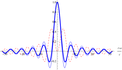
Figure 1: Comparison of sinc (bold), $\tilde{\mathrm{S}}_{1}$, and $\tilde{\mathrm{S}}_{0}$ (dashed). Sinc and $\tilde{\mathrm{S}}_{1}$ are extremely qualitatively similar, both being unity at zero whereas $\mathrm{S}_{0}$ vanishes at zero.

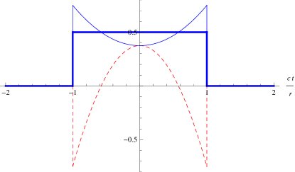
Figure 2: The same functions as in Fig. 1, but in the time domain: the rectilinear distribution (bold), S₀, and S₁ (dashed).

III.1 Dissipation and Damping with $\mathbf{A}$-coupling

To describe quasirelativistic damping, we can integrate by parts the $\mathbf{A}$-coupling dissipation kernel to obtain terms corresponding to damping, mass renormalization, and dissipationless backreaction. In the quasirelativistic regime we treat the positions $\mathbf{x}$ as quasistatic within the convolution (as discussed in App. B)

$$(\boldsymbol{\mu}_{ij}^{A}\!\ast\mathbf{z})(t)=\int_{0}^{t}\!\!dt^{\prime}\boldsymbol{\mu}_{\!A}[\mathbf{x}_{i}(t)\!-\!\mathbf{x}_{j}(t^{\prime});t\!-\!t^{\prime}]\,\mathbf{z}(t^{\prime})\,,$$

where $\mathbf{z}(t)$ is some arbitrary source. Integrating by parts, and neglecting the intrinsic time dependence in the positions (which is equivalent to ignoring higher-order corrections in $v/c$), gives

$$(\boldsymbol{\mu}_{ij}^{A}\!\ast\mathbf{z})(t) =(\boldsymbol{\gamma}_{ij}^{A}\!\ast\dot{\mathbf{z}})(t)-\boldsymbol{\gamma}_{\!A}[\mathbf{x}_{i}(t)\!-\!\mathbf{x}_{j}(t);0]\,\mathbf{z}(t)$$

$$+\boldsymbol{\gamma}_{\!A}[\mathbf{x}_{i}(t)\!-\!\mathbf{x}_{j}(0);t]\,\mathbf{z}(0)\,,$$

where the final term is a transient slip. Although the slip evolution arises during the same period of time as the conventional Abraham-Lorentz acausality, its role is well understood from QBM studies where it has been shown to be unproblematic (see App. A and Ref. Fleming et al. (2011a) where the initial evolution for initial factorized system plus environment states in terms of so-called “slip” and “jolt” evolution is reviewed). It may therefore be discarded for our purposes; doing so is equivalent to choosing an initial state which is more properly correlated to the environment. The difference between QBM and QED is that with the relativistic field, not only are there instantaneous self-transients from $\boldsymbol{\gamma}_{ii}(t)$, there are also retarded cross-transients from $\boldsymbol{\gamma}_{ij}(t)$. Figure 2 shows that the electrodynamic slip only produces a transient effect for $t<r/c$. Essentially, for factorized states of the particles and field, the particles are completely unaware of each other’s existence until photons travel between them and suddenly (and violently) establish correlations at their first mediation.

Unlike QBM, $\boldsymbol{\gamma}_{A}[\mathbf{r}_{ij}(t);0]$ contains both self interactions, which renormalize the mass, and field-mediated interactions. Using Eq. (34), this term becomes

$$\boldsymbol{\gamma}_{\!A}[\mathbf{r};0]=\frac{3}{4}c\,\gamma_{0}\frac{1+\hat{\mathbf{r}}\,\hat{\mathbf{r}}^{\mathrm{T}}}{|\mathbf{r}|}\,,$$

and we see the emergence of the Darwin Hamiltonian (e.g. see Jackson Jackson (1998) Sec. 12.7). The magnetostatic energy of the Darwin Hamiltonian (which is classical) is given by

$$\mathbf{V}_{ij}=-2\frac{e_{i}}{m_{j}}\mathbf{p}_{i}^{\mathrm{T}}\boldsymbol{\gamma}_{\!A}[\mathbf{r}_{ij};0]\frac{e_{j}}{m_{j}}\mathbf{p}_{j}\,.$$

The quantum extension of the Darwin Hamiltonian requires an operator-ordering prescription that our analysis will provide upon applying these results to the Langevin equation.

These results exemplify how the equations of motion that result from an $\mathbf{A}$-coupling interaction give consistent formulas for damping and backreaction, despite the noise being problematic as previously discussed.

III.2 Dissipation and Damping with Electric-Dipole Coupling

In this subsection we describe the sense in which the electric-dipole interaction gives a less desirable description of damping and backreaction, despite providing a consistent description of thermal noise, as previously described. For $\pi$-coupling to the field, the dissipation kernel is approximately given by

$$\boldsymbol{\mu}_{\mbox{\normalsize$\pi$}}[\mathbf{x}(t),\mathbf{y}(t^{\prime});t,t^{\prime}]\approx\left\langle\frac{1}{2\imath\hbar}\left[\!\left[\underline{\boldsymbol{\mbox{\Large$\pi$}}}(\mathbf{x}(t),t),\underline{\boldsymbol{\mbox{\Large$\pi$}}}(\mathbf{y}(t^{\prime}),t^{\prime})\right]\!\right]\right\rangle_{\mathrm{\!\!env}},$$

with the same $\mathcal{O}\left(\hbar^{2}/c^{3}\right)$ phase discrepancies discussed in App. B. The $\pi$-coupling dissipation kernel is related to the $\mathbf{A}$-coupling dissipation kernel via

$${\boldsymbol{\gamma}}_{\mbox{\normalsize$\pi$}}[\mathbf{r};t,t^{\prime}] =-\frac{\partial^{2}}{\partial t^{\prime 2}}\,{\boldsymbol{\gamma}}_{\!A}[\mathbf{r};t,t^{\prime}]\,,$$ (43)

$$\tilde{\boldsymbol{\gamma}}_{\mbox{\normalsize$\pi$}}[\mathbf{r};\omega] =\omega^{2}\,\tilde{\boldsymbol{\gamma}}_{\!A}[\mathbf{r};\omega]\,.$$ (44)

This result is equivalent to dissipation from a supra-Ohmic bath in QBM. As an integration kernel ${\boldsymbol{\gamma}}_{\mbox{\normalsize$\pi$}}$ is relatively pathological and must be integrated by parts twice to obtain the well-behaved kernel ${\boldsymbol{\gamma}}_{A}$. Such an integration is straightforward for the single-particle theory in the dipole approximation, but for the multiparticle and higher-order relativistic theory this generates many additional terms and limits which must be carefully analyzed in constructing the Langevin equation. Although, with care, it should be possible to proceed this way, the approach in the next section is clearer and more straightforward.

III.3 Standard Dipole Calculation

Before presenting our effective equations of motion in Sec. IV, we first review the derivation of the standard results for a single particle. Taking the dipole approximation we drop all position dependence in the integration kernels. Substituting Eq. (30) (integrated by parts once) into Eqs. (26)-(27) we obtain the Langevin equation

$$m\ddot{\mathbf{x}}(t)=-e\boldsymbol{\nabla}\phi(\mathbf{x})-2\,e^{2}\,({\gamma}^{\mbox{\normalsize$\pi$}}\ast\dot{\mathbf{x}})(t)+e\,\boldsymbol{\xi}^{\mbox{\normalsize$\pi$}}(t)\,,$$ (45)

discarding the transient terms. This equation of motion is runaway free for bare mass $m>0$ as reviewed in App. A.5.

Integrating-by-parts the $\pi$-damping integral in the Langevin equation (45) two times, to obtain $A$-coupling damping, discarding additional transient terms, and grouping like terms, we obtain the standard Abraham-Lorentz-Langevin equation

$$m_{\mathrm{ren}}\ddot{\mathbf{x}}(t) =-e\boldsymbol{\nabla}\phi(\mathbf{x})+2\,e^{2}(\gamma^{A}\ast\dddot{\mathbf{x}})(t)-e\,\dot{\boldsymbol{\xi}}^{A}(t)\,,$$ (46)

$$m_{\mathrm{ren}} =m+2\,e^{2}\gamma^{A}(0),$$ (47)

where $m_{\text{ren}}$ is the renormalized particle mass. The same result is obtained by integrating-by-parts the dissipation integral in the Langevin equations (20)-(21). Note that $(\gamma^{A}\ast\dddot{\mathbf{x}})(t)\approx\gamma_{0}\,\dddot{\mathbf{x}}(t)$ in the high cutoff (“point-particle”) limit. Positive bare mass $m,$ which is required for runaway-free motion, requires a finite cutoff $\Lambda$ in the field modes such that $2\,e^{2}\gamma^{A}(0)<m_{\mathrm{ren}}\,,$ noting that $\gamma^{A}(0)\propto\gamma_{0}\,\Lambda$. Therefore positive bare mass requires an ultraviolet cutoff $\Lambda,$ or equivalently a form factor that cuts off the particle field coupling, on the order of $\varepsilon_{0}c^{3}m_{\mathrm{ren}}/e^{2}$ or smaller. This is directly seen from our stability analysis in App. A.5, or simply by noting that with a negative bare mass the system + environment Hamiltonian no longer has a lower bound in its energy spectrum.

IV $1/c$ Expansion of QED

In the previous section, we contrasted how the standard results are obtained when the interaction is expressed in terms of either $\dot{\mathbf{x}}\cdot\mathbf{A}$ or $\mathbf{x}\cdot\boldsymbol{\mbox{\Large$\pi$}}$ coupling. We have highlighted the problem of simultaneously obtaining well-behaved noise and backreaction. In Ford and O’Connell (1991), Ford and O’Connell showed that the equations of motion for a charged particle with structure can be order-reduced to obtain the structure-independent equation of motion

$$m\ddot{\mathbf{x}}=\left\{1+\frac{2\,e^{2}\gamma_{0}}{m}\frac{d}{dt}\right\}\left[\mathbf{F}_{\mathrm{ext}}(\mathbf{x})-e\,\dot{\boldsymbol{\xi}}(t)\right]\,,$$ (48)

which is accurate to lowest order in the timescale

$$\tau_{m}=e^{2}/6\pi\varepsilon_{0}mc^{3}\sim\alpha\hbar/mc^{2}\,,$$ (49)

where $\alpha=e^{2}/4\pi\varepsilon_{0}\hbar c$ is the fine-structure constant. For bound states, this is equivalent to the dimensionless order $\alpha\,\Delta E/mc^{2}$, where $\Delta E$ denotes the relevant energy-level transitions of the system. For driving forces, the expansion parameter is $\alpha\,\hbar\omega/mc^{2}$, given a driving frequency $\omega$. In either case the result is of order $1/c^{3}$, and the $e^{3}\dot{\boldsymbol{\xi}}$ term is negligible given the approximations which have been made in constructing this equation.

Eq. (48) is causal, runaway-free, and is in general dissipative (i.e. accelerated motion is damped). The Ford and O’Connell result is generic in the sense that any particle, with reasonable assumptions about its structure (form factor), will have backreaction of this form in the weak-backreaction limit. In this sense, the result is the universal (effective) low-energy, and equivalently lowest order in $1/c$, result for backreaction. Below, we obtain stochastic equations of motion with damping consistent with Eq. (48), but from a different approach that provides additional insights into the nature of backreaction. Whereas the more-standard approach of Ford and O’Connell considers Eq. (1) to be of order $\mathcal{O}(1/c^{3})$ and their Eq. (48) to be order reduced, our approach will generate equivalent damping to Eq. (48) which is strictly $\mathcal{O}(1/c^{3})$, and not order reduced. Within our analysis, the standard Eq. (1) is mixed-ordered, and this is the primary source of its pathological behaviors. An advantage of our method is that it allows for a consistent and systematic extension to higher orders which includes both higher-order relativistic corrections, and higher-order effects of backreaction.

Our approach fundamentally relies upon consistent application of a dimensionful $1/c$ expansion around the Hamiltonian

$$\mathbf{H}_{\text{NR}}=\sum_{i}\frac{\mathbf{p}_{i}^{2}}{2m_{i}}+\sum_{i<j}\frac{1}{4\pi\varepsilon_{0}}\frac{e_{i}e_{j}}{\left|\mathbf{r}_{ij}\right|}\,,$$

which is viewed as the lowest-order, “nonrelativistic” Hamiltonian in this approach. All of the additional terms that arise in the QED Hamiltonian are then viewed as perturbations, whose order is based on the powers of $1/c$.

We begin with the $\mathbf{A}$-coupling, Coulomb-gauge Hamiltonian in (17). From the previous analysis we observe that the self-field generates, at lowest order $\mathcal{O}(1/c^{2}),$ magnetostatic and renormalization terms (see Sec. III.1). Because our approximation is based on a systematic expansion in powers of $1/c,$ and here we work to $\mathcal{O}(1/c^{3}),$ we effectively drop the $\mathbf{A}^{2}$ system-field interaction terms in the Hamiltonian. These neglected terms are all of order $(v/c)^{4}$, $\alpha\,(\Delta E/mc^{2})\,(v/c)^{2}$, and so, making them $\mathcal{O}(1/c^{4})$. For now we assume the usual nonrelativistic kinetic energy for the particles, but for consistency we include the relativistic corrections at the appropriate order in Sec. IV.3. Therefore, the consistent $\mathcal{O}(1/c^{3})$ effective Hamiltonian in the Coulomb gauge is

$$\mathbf{H}_{\mathrm{EQED}}=\sum_{i}\left\{\frac{\mathbf{p}_{i}^{2}}{2m_{i}}+e\,\phi(\mathbf{x}_{i})\right\}$$ (50)

$$-\sum_{i}\frac{e_{i}}{2m_{i}}\left\{\mathbf{p}_{i}\cdot\mathbf{A}(\mathbf{x}_{i})+\mathbf{A}(\mathbf{x}_{i})\cdot\mathbf{p}_{i}\right\}+\mathbf{H}_{\mathrm{field}}+\mathcal{O}(1/c^{4})\,.$$

The Heisenberg equations of motion for the system driven by the field for the effective Hamiltonian $\mathbf{H}_{\mathrm{EQED}}$ are

$$\dot{\mathbf{x}}_{i} =\frac{\mathbf{p}_{i}}{m_{i}}-\frac{e_{i}}{m_{i}}\mathbf{A}(\mathbf{x}_{i})\,,$$ (51)

$$\dot{\mathbf{p}}_{i} =-e_{i}\boldsymbol{\nabla}_{\!\!i}\phi(\mathbf{x}_{i})+\frac{e_{i}}{2m_{i}}\boldsymbol{\nabla}_{\!\!i}\left\{\mathbf{p}_{i}\cdot\mathbf{A}(\mathbf{x}_{i})+\mathbf{A}(\mathbf{x}_{i})\cdot\mathbf{p}_{i}\right\}\,,$$ (52)

and the Heisenberg equations of motion for the environment driven by the system are

$$\dot{\mathbf{A}}_{\mathbf{k},\boldsymbol{\epsilon}_{k}} =\frac{1}{\varepsilon_{0}}\boldsymbol{\mbox{\Large$\pi$}}_{\mathbf{k},\boldsymbol{\epsilon}_{k}}+\frac{1}{\varepsilon_{0}\omega_{k}}\sum_{j}\frac{e_{j}}{2m_{j}}\left\{\sin(\mathbf{k}\cdot\mathbf{x}_{j}),{\mathbf{p}}_{j}\right\}\,,$$ (53)

$$\dot{\boldsymbol{\mbox{\Large$\pi$}}}_{\mathbf{k},\boldsymbol{\epsilon}_{k}} =-\varepsilon_{0}\omega_{k}^{2}\,\mathbf{A}_{\mathbf{k},\boldsymbol{\epsilon}_{k}}+\sum_{j}\frac{e_{j}}{2m_{j}}\left\{\cos(\mathbf{k}\cdot\mathbf{x}_{j}),{\mathbf{p}}_{j}\right\}\,.$$ (54)

As derived in App. B, the driven solution expressed in manifestly-Hermitian form is

$$\mathbf{A}(\mathbf{x}_{i},t)=\boldsymbol{\xi}_{i}^{A}(t)-\sum_{j}\frac{e_{j}}{m_{j}}\left\{(\boldsymbol{\mu}_{ij}^{A}\ast{\mathbf{p}}_{j})(t)+(\boldsymbol{\mu}_{ij}^{A}\ast{\mathbf{p}}_{j})^{\dagger}(t)\right\}\,,$$ (55)

where the $\boldsymbol{\xi}_{i}(t)$ are uncorrelated processes for $i\neq j$. Following the approach in Sec. III.1, integrating the dissipation kernel by parts gives

$$\mathbf{A}[\mathbf{x}_{i}(t),t]=\boldsymbol{\xi}_{i}(t)-2\frac{e_{i}}{m_{i}}\gamma_{0}\,\dot{\mathbf{p}}_{i}(t)$$ (56)

$$+\sum_{j}\left\{\boldsymbol{\gamma}[\mathbf{r}_{ij}(t);0]\frac{e_{j}}{m_{j}}\mathbf{p}_{j}(t)+\left(\boldsymbol{\gamma}[\mathbf{r}_{ij}(t);0]\frac{e_{j}}{m_{j}}\mathbf{p}_{j}(t)\right)^{\!\dagger}\right\},$$

Here we have neglected the transient slip terms (which, as noted before and as is reviewed in the appendix, can be verified to not induce runaways or acausal behavior) and corrections of higher order in $v/c$.

Substituting the driven field solution into the system equations of motion gives the renormalized multiple-particle Langevin equation

$$\dot{\mathbf{x}}_{i}=\; \frac{\mathbf{p}_{i}}{m_{i}}-\frac{e_{i}}{m_{i}}\boldsymbol{\xi}_{i}+2\frac{e_{i}^{2}}{m_{i}^{2}}\gamma_{0}\,\dot{\mathbf{p}}_{i}+\boldsymbol{\nabla}_{\!\!\mathbf{p}_{i}}\sum_{j\neq i}\mathbf{V}_{ij}\,,$$ (57)

$$\dot{\mathbf{p}}_{i}=\; -e_{i}\boldsymbol{\nabla}_{\!\!\mathbf{x}_{i}}\phi(\mathbf{x}_{i})-\boldsymbol{\nabla}_{\!\!\mathbf{x}_{i}}\sum_{j\neq i}\mathbf{V}_{ij}\,,$$ (58)

Details of the renormalization will be explained further in Sec. IV.2. The quantum magnetostatic potential $\mathbf{V}$ is given by

$$\mathbf{V}_{ij} =-\frac{1}{2}\frac{e_{i}}{m_{i}}\frac{e_{j}}{m_{j}}\left[\mathbf{p}_{i}^{\mathrm{T}}\boldsymbol{\gamma}[\mathbf{r}_{ij};0]\,\mathbf{p}_{j}+\mathbf{p}_{j}^{\mathrm{T}}\boldsymbol{\gamma}[\mathbf{r}_{ji};0]\,\mathbf{p}_{i}\right]$$

$$-\frac{1}{2}\frac{e_{i}}{m_{i}}\frac{e_{j}}{m_{j}}\mathrm{Tr}_{x}\!\left[\mathbf{p}_{i}\,\mathbf{p}_{j}^{\mathrm{T}}\,\boldsymbol{\gamma}[\mathbf{r}_{ij};0]+\boldsymbol{\gamma}[\mathbf{r}_{ij};0]\,\mathbf{p}_{i}\,\mathbf{p}_{j}^{\mathrm{T}}\right]\,.$$ (59)

The last two terms have been expressed with a spatial trace

$$\mathrm{Tr}_{x}[\mathbf{M}]\equiv M_{xx}+M_{yy}+M_{zz}\,,$$ (60)

to keep the proper Hilbert-space operator ordering. The complexity of this expression is due to the non-commutativity from both Hilbert-space and spatial (3-vector and 3$\times$3 matrix) operations. This quantum magnetostatic potential is consistent with the (classical) Darwin magnetostatic potential (also see Sec. III.1)

$$\mathbf{V}_{ij} =-2\frac{e_{i}}{m_{i}}\mathbf{p}_{i}^{\mathrm{T}}\boldsymbol{\gamma}[\mathbf{r}_{ij};0]\frac{e_{j}}{m_{j}}\mathbf{p}_{j}\,,$$ (61)

$$\boldsymbol{\gamma}[\mathbf{r};0] =\frac{3}{4}c\,\gamma_{0}\frac{1+\hat{\mathbf{r}}\,\hat{\mathbf{r}}^{\mathrm{T}}}{r}\,.$$ (62)

Moreover, the operator ordering in Eq. (59) is consistent with the Breit equation for spin-$1/2$ particles Breit (1930) (often named “orbit-orbit interaction” in that context), when one ignores all of the Pauli spin matrices.

Equations (57)-(58) are one of the main results of this paper. They are multiparticle stochastic equations of motion consistent through order $\mathcal{O}\!\left(1/c^{3}\right)$ in the field influences with, as we will show, stable (runaway-free) backreaction even as the field cutoff goes to infinity. [$\mathcal{O}\!\left(1/c^{3}\right)$ kinematics will be given in Sec. IV.3.] Notice that our results show that the mass renormalization associated with the dissipative backreaction, at $\mathcal{O}\!\left(1/c^{3}\right),$ is due to magnetostatic self-interactions. Our effective Hamiltonian treatment also correctly produces the second-order magnetostatic corrections without extraneous fourth-order terms (as Breit accidentally included in his first calculation Breit (1929, 1930)). This result is not present in the standard treatments.

Our analysis suggests that the pathologies of the standard Abraham-Lorentz equations can be viewed, from the perspective of a $1/c$ effective theory expansion, as a consequence of performing a mixed-order calculation. In terms of a $1/c$ expansion starting from the Coulomb-gauge Hamiltonian, there are $\mathcal{O}\!\left(1/c^{4}\right)$ multipole-expansion terms in the $\mathbf{p\cdot A}\!\left(\mathbf{x}\right)$ interaction terms that are of the same order as the lowest-order dipole terms present in the $\mathbf{A}\!\left(\mathbf{x}\right)^{2}$ interaction. This reveals that uniform application of the dipole approximation by itself to the Coulomb gauge Hamiltonian is inconsistent with the $1/c$ expansion, in the sense that it keeps some terms of $\mathcal{O}\!\left(1/c^{4}\right)$, but discards others. For a consistent $\mathcal{O}\!\left(1/c^{3}\right)$ expansion, effectively the dipole approximation to the $\mathbf{p\cdot A}\!\left(\mathbf{x}\right)$ interaction is kept and the $\mathbf{A}\!\left(\mathbf{x}\right)^{2}$ interaction is dropped entirely, as we have done.

Historically, the Abraham-Lorentz equation has most often not been viewed perturbatively, but instead as an effort to obtain an exact, nonrelativistic point-particle result. Our philosophy has been to instead look for a consistent low-energy, effective theory from the beginning. Giving up any claim to an exact solution, we gain new insight into how a perturbatively consistent solution arises within a framework that can be systematically extended to higher orders. An alternative approach is to apply order reduction to the standard result, which can be iterated into the Ford-O’Connell equation (48), with additional backreaction contributions of higher order in $1/c$ (and higher-order derivatives). One then discards these higher-order terms in the name of order reduction. Combining our relations (57) and (58) reproduces the same damping as the Ford-O’Connell equation, however, without any higher-order terms to be order reduced. Thus, in terms of a $1/c$ expansion, the damping in the Ford-O’Connell equation is strictly $1/c^{3}$ (and thus consistent), whereas the pathological backreaction in the Abraham-Lorentz equation is of mixed order. There is an interesting parallel here to Breit’s original calculation Breit (1929), where pathological equations resulted when Breit accidentally included a fourth-order operator in a calculation which was only accurate to second order.

IV.1 Noise and backreaction stability

As previously discussed in Section II.1 the “noise” for the standard ${\mathbf{v}}\cdot\mathbf{A}$ coupling Langevin equation cannot be independently sampled from a thermal distribution. The standard calculation only gives well-behaved noise within the electric-dipole gauge. In contrast, our analysis, to order $\mathcal{O}\!\left(1/c^{3}\right)$ starting from the Coulomb gauge, gives well-behaved noise and dissipation. Comparing the derivations in Sections II.1 and IV, we see that our noise and the standard electric-dipole gauge noise only differ by contributions from the $\mathbf{A}\!\left(\mathbf{x}\right)^{2}$ interaction of the order $1/c^{4}$ and higher, or more specifically $(v/c)^{4}$, $\alpha\,(\Delta E/mc^{2})\,(v/c)^{2}$, etc..

It is interesting to consider further why the noise in the standard (mixed-order) Coulomb gauge calculation is problematic. Examining Eq. (24), we see that the backreaction (which depends on velocity ${\mathbf{v}}$ in this expression) contains some perturbative amount of the “$\mathbf{p}$-noise”, which is true thermal noise, obtained in our calculation. Similarly, inspection also shows that the noise in the standard (mixed-order) Coulomb gauge calculation contains some perturbative amount of “$\mathbf{p}$-backreaction”, which is the resistive damping that accompanies thermal noise, obtained in our calculation. In other words, the (non-thermal) noise in the standard (mixed-order) Coulomb gauge calculation contains some backreaction, and the backreaction contains some noise. Therefore, even in the classical limit of (24) we would have to enforce an artificial constraint upon the $\mathbf{p}$-backreaction implying that the backreaction in the Coulomb gauge includes a non-zero average value of the $\mathbf{p}$-noise.

The physics may be clearer from another perspective. Recalling that $m\mathbf{v}=\mathbf{p}-e\mathbf{A}$ such that the velocity $\mathbf{v}$ depends on both the particle and field canonical coordinates, we see that velocity driving entails that the field is driven by both the system (particle) and itself. In other words, velocity driving of the field implies a perturbative feedback loop in the environment dynamics. Essentially, the field can self-generate stronger and stronger field excitations, albeit at an order beyond which the theory is accurate, and this can result in runways. In contrast, in our new equations of motion, Eq. (55), the field is driven by the canonical momentum $\mathbf{p}$ rather than the velocity $\mathbf{v}$, and such pathological processes do not occur.

Our next task is to demonstrate that the equations of motion are nonperturbatively stable. When combined, relations (57) and (58) reproduce the same damping as the Ford-O’Connell equation (48), which is already known to be stable, and the noises are perturbatively consistent. We can gain additional insight, however, by comparing our analysis to the analysis leading to (48). In this paper, we begin with an effective Hamiltonian, and work consistently to $\mathcal{O}\!\left(1/c^{3}\right).$ With regard to the self-force this is essentially equivalent to taking both the dipole approximation and neglecting the $\mathbf{A}^{2}$ term in the Hamiltonian. At $\mathcal{O}\!\left(1/c^{3}\right)$, we find that there is no constraint on the cutoff and the backreaction is fully insensitive to particle structure. In contrast, in (48) the dipole approximation is made to the full Hamiltonian including the $\mathbf{A}^{2}$ term, and instead a particle-structure form factor is assumed, which gives an effective cutoff in the particle-field interaction. The equations of motion are then order reduced, effectively to $\mathcal{O}\!\left(1/c^{3}\right)$, and the resulting structure-independent equations of motion are found to be runaway free. The ultimate agreement between these approaches is consistent with the fact that the contribution to backreaction from the $\mathbf{A}^{2}$ term in the Hamiltonian is effectively negligible in the regime where the two methods of approximation are valid.

Although it is already known that Eq. (48) is runaway free and causal, we now re-analyze these properties within the present framework to see how this physics arises from with a purely effective theory framework. We will show that the dynamics of the open system are dissipative and stable in a manner analogous to the QBM analysis given in App. IV.1. Consider a single particle and denote the system Hamiltonian

$$\mathbf{H}_{\mathrm{sys}}\equiv\frac{\mathbf{p}^{2}}{2m}+e\,\phi(\mathbf{x})\,.$$

An energy constraint can be obtained from either the Heisenberg equations of motion for $\mathbf{H}_{\mathrm{sys}}(t)$ or by integrating the (classical) Langevin equation (69) along with the second (70). Discarding the irrelevant transient terms (which can be shown to be bounded and runaway-free) we obtain the relation

$$\mathbf{H}_{\mathrm{sys}}(t)=\mathbf{H}_{\mathrm{sys}}(0)+\mathbf{H}_{\gamma}(t)+\mathbf{H}_{\xi}(t)\,,$$

where

$$\mathbf{H}_{\gamma}(t)=-2\frac{e^{2}}{m^{2}}\gamma_{0}\int_{0}^{t}\!\!dt^{\prime}\,\dot{\mathbf{p}}\!\left(t^{\prime}\right)^{2}$$ (63)

is the energy lost to damping and

$$\mathbf{H}_{\xi}(t)=\frac{e}{m}\int_{0}^{t}\!\!dt^{\prime}\frac{1}{2}\left\{\boldsymbol{\xi}(t^{\prime})\cdot\dot{\mathbf{p}}(t^{\prime})+\dot{\mathbf{p}}(t^{\prime})\cdot\boldsymbol{\xi}(t^{\prime})\right\}$$ (64)

is the work done by the noise $\boldsymbol{\xi}(t^{\prime}).$ The contribution from damping is manifestly a negative quantity. The noise is random and may do positive or negative work, but the damping only removes energy from the system (and delivers it to the environment and interaction). At least at this order, the damping is strictly local and so energy is lost to dissipation in a strictly uniform manner.

It is important to note that the system here is given by the canonical variables $\left(\mathbf{x,p}\right)$, and $\mathbf{H}_{\mathrm{sys}}$ does not correspond to the mechanical energy of the particle, for the same reason that $\mathbf{p}^{2}/2m$ is not the mechanical kinetic energy. From Eq. (20) the velocity and momentum differ by the vector potential, which includes both backreaction and noise. If the system momentum $\mathbf{p}$ relaxes under dissipative motion, then so does $\dot{\mathbf{p}}$ and by extension the backreaction $\gamma_{0}\,\dot{\mathbf{p}}$. Given noise, the system velocity fluctuates around the average

$$\left\langle m\,\mathbf{v}\right\rangle_{\boldsymbol{\xi}}=\left\langle\mathbf{p}+2\frac{e^{2}}{m}\gamma_{0}\,\dot{\mathbf{p}}\right\rangle_{\!\!\boldsymbol{\xi}}\,,$$ (65)

implying that the system velocity is damped. If no external forces are applied, the canonical and mechanical momenta approach each other (on average) in the late-time limit.

IV.2 Mass Renormalization

In our Langevin equations (57)-(58), the $\mathbf{p}^{2}/2m$ mass renormalization takes the form of magnetostatic self-interaction, which is ordinarily discarded in classical electrodynamics. Here we examine the counter terms involved in the renormalization and contrast them to the standard mass renormalization previously discussed in Sec. III.3.

Consider most simply the single particle theory in the dipole approximation. The resultant open-system equations of motion are then given by

$$\dot{\mathbf{x}}(t) =\frac{\mathbf{p}(t)}{m_{\mathrm{ren}}}+2\frac{e^{2}}{m_{\mathrm{bare}}^{2}}\gamma_{0}\,\dot{\mathbf{p}}(t)-\frac{e}{m_{\mathrm{bare}}}\,\boldsymbol{\xi}(t)\,,$$ (66)

$$\dot{\mathbf{p}}(t) =-e\boldsymbol{\nabla}\phi(\mathbf{x})\,,$$ (67)

in terms of the renormalized mass

$$\frac{1}{m_{\mathrm{ren}}}=\frac{1}{m_{\mathrm{bare}}}+2\frac{e^{2}}{m_{\mathrm{bare}}^{2}}\gamma(0)\,.$$ (68)

Consistent with this order of perturbative analysis, we may express our Langevin equations as

$$\dot{\mathbf{x}}(t) =\frac{\mathbf{p}(t)}{m_{\mathrm{ren}}}+2\frac{e^{2}}{m_{\mathrm{ren}}^{2}}\gamma_{0}\,\dot{\mathbf{p}}(t)-\frac{e}{m_{\mathrm{ren}}}\,\boldsymbol{\xi}(t)\,,$$ (69)

$$\dot{\mathbf{p}}(t) =-e\boldsymbol{\nabla}\phi(\mathbf{x})\,.$$ (70)

In this perspective, the renormalization of the $\mathbf{p}^{2}/2m$ mass and the $e/m\,(\mathbf{p}\cdot\mathbf{A})$ mass enter at different orders.

It is well known that the instability of the Abraham-Lorentz equation arises from its implied negative bare mass for the system, which in-turn comes about if the high frequency cutoff $\Lambda$ (or reciprocal radius $c/r$) exceeds the characteristic frequency $\tau_{m}^{-1}$ Ford and O’Connell (1991); Moniz and Sharp (1977). Yet to lowest order in $\tau_{m}$ (equivalently $1/c^{3}$), the dynamics of charged-particle motion is insensitive to the high-energy details of the theory and is thus not problematic in that regime Ford and O’Connell (1991). It is therefore not surprising that our perturbative approach yields cutoff-insensitive behavior, however, the manner in which cutoff sensitivity is avoided is interesting. Whereas the standard radiation-reaction calculations involve a mass renormalization of $m\mathbf{v}^{2}/2$ given by Eq. (68), which runs the bare mass to negative infinity in the high cutoff limit, our calculation runs the bare mass to positive zero in the high cutoff limit, and no pathological behavior is induced for any finite cutoff.

IV.3 Relativistic Kinematics

For consistency in our quasirelativistic expansion of $1/c$, we should include the relativistic corrections to the single particle kinetic energy, as is standard in the Darwin Hamiltonian. Expanding the relativistic kinetic energy gives

$$\mathbf{H}_{\mathrm{rel}} =c\,\sqrt{(mc)^{2}+\left(\mathbf{p}-e\,\mathbf{A}\right)^{2}}\,,$$ (71)

$$\approx mc^{2}+\frac{\left(\mathbf{p}-e\,\mathbf{A}\right)^{2}\!\!}{2m}-\frac{\left(\mathbf{p}-e\,\mathbf{A}\right)^{4}\!\!}{8m^{3}c^{2}}+\cdots\,,$$ (72)

keeping terms of order $\mathcal{O}(1/c^{2})$. In the absence of external fields, this generates a second-order correction to Eq. (57) giving

$$\dot{\mathbf{x}}(t)=\left[1-\frac{1}{2}\left(\frac{\mathbf{p}(t)}{mc}\right)^{2}\right]\frac{\mathbf{p}(t)}{m}+2\frac{e^{2}}{m^{2}}\gamma_{0}\,\dot{\mathbf{p}}(t)-\frac{e}{m}\,\boldsymbol{\xi}(t)\,,$$ (73)

and otherwise the Langevin equations are identical. As in the Darwin Hamiltonian, this relativistic correction must be considered perturbatively. At the present order of perturbation theory, however, we can resum the term into the free velocity

$$\left[1-\frac{1}{2}\left(\frac{\mathbf{p}}{mc}\right)^{2}\right]\frac{\mathbf{p}}{m}=\frac{\frac{\mathbf{p}}{m}}{\sqrt{1+\left(\frac{\mathbf{p}}{mc}\right)^{2}}}+\mathcal{O}\!\left(\frac{1}{c^{4}}\right)\,,$$

which is more convenient and better behaved in the equations of motion. This can also be done in the effective Hamiltonian to ensure that the energy spectrum has a lower bound.

Note that even nonperturbatively these kinematic corrections included in the stability analysis given in Sec. IV.1 will still yield dissipative backreaction, as all of these terms commute with the $\mathbf{A}\cdot\mathbf{p}$ interaction at the relevant order. The only modification will be in the definition of the canonical system Hamiltonian (now relativistic), and the noise average of the velocity will be given by

$$\left\langle m\,\mathbf{v}\right\rangle_{\boldsymbol{\xi}}=\left\langle\frac{\mathbf{p}}{\sqrt{1+\left(\frac{\mathbf{p}}{mc}\right)^{2}}}+2\frac{e^{2}}{m}\gamma_{0}\,\dot{\mathbf{p}}\right\rangle_{\!\!\!\!\boldsymbol{\xi}}\,.$$ (74)

IV.4 Electromagnetic Damping is Relativistic

The standard Abraham-Lorentz equation (1) is commonly referred to as “nonrelativistic”. Within the framework of a $1/c$ expansion, this equation is more accurately described as quasirelativistic. From this perspective, the damping force, which is $\mathcal{O}(1/c^{3}),$ is intrinsically a relativistic correction to the particle dynamics. Let us reexpress the $(v/c)^{2}$ magnetostatic and $1/c^{3}$ damping forces in Eq. (57) as both arising from dynamical generators

$$\dot{\mathbf{x}}_{i}=\; \frac{\mathbf{p}_{i}}{m_{i}}-\frac{e_{i}}{m_{i}}\boldsymbol{\xi}_{i}+\boldsymbol{\nabla}_{\!\!\mathbf{p}_{i}}\left\{\boldsymbol{\Gamma}_{i}+\sum_{j\neq i}\mathbf{V}_{ij}\right\},$$ (75)

$$\boldsymbol{\Gamma}_{i} \equiv\frac{d}{dt}\left(\frac{e_{i}}{m_{i}}\mathbf{p}_{i}^{\mathrm{T}}\gamma_{0}\frac{e_{i}}{m_{i}}\mathbf{p}_{i}\right)\,.$$ (76)

By comparison with Eq. (61)-(62), if the magnetostatic potential $\mathbf{V}$ is considered $(v/c)^{2}$, then the damping generator $\boldsymbol{\Gamma}$ is of relative order $(r/c)(d/dt)(v/c)^{2}$. Thus the damping force can be interpreted as a more dynamical and more relativistic correction. Given that both of these generators arise from the same integration kernel without the full dipole approximation (see App. B), a higher-order “multipole” expansion in $1/c$ can expect to include many more such terms of higher order. The relativistic nature of the expansion terms will be even clearer at higher orders.

V Summary and Discussions

We have derived new stochastic equations of motion (57)-(58) & (73) for multiple charged particles in the electromagnetic field. These equations of motion incorporate the known relativistic corrections to the electrodynamics of spinless charged particles to order $\mathcal{O}(1/c^{3})$, including the electrostatic, magnetostatic, electromagnetic damping forces, and field fluctuations. Moreover the equations of motion are manifestly causal and runaway-free. Our analysis shows that a $1/c$ expansion to the Coulomb-gauge Hamiltonian describes consistent and well-behaved nonequilibrium electrodynamics for spinless charged particles. Our consistent-order equations of motion have a close correspondence with the order-reduced Ford-O’Connell equation, which is known to be well behaved. Whereas traditionally the Abraham-Lorentz equation has been considered an “exact nonrelativistic” equation, from the perspective of our analysis, pathologies in the standard Abraham-Lorentz equation are associated with inconsistent, mixed-order in $1/c$, approximations. Our view is that radiation reaction is intrinsically relativistic, though the Abraham-Lorentz equation may only fully capture its effect to lowest order in $1/c$, and the order reduction used in deriving the Ford-O’Connell equation actually serves to rid the dynamics of inappropriate mixed-order contributions.

At $\mathcal{O}\!\left(1/c^{3}\right)$, mass renormalization is identified with the magnetostatic self-interaction and, at this order, the bare mass is positive for all cutoffs and the backreaction is fully insensitive to particle structure. An interesting question for future research is whether the cutoff insensitivity is preserved at higher-orders in the $1/c$ expansion, as to our knowledge no rigorously-derived relativistic equations of motion exist in the literature. For a single particle, we see that only at $\mathcal{O}\!\left(1/c^{4}\right)$ does the (dipole approximation to the) $\mathbf{A}\!\left(\mathbf{x}\right)^{2}$ interaction play a role, but at the same order multipole terms in the $\mathbf{p\cdot A}\!\left(\mathbf{x}\right)$ interaction must also be included for consistency. The standard results show that inclusion of the $\mathbf{A}\!\left(\mathbf{x}\right)^{2}$ interaction plus dipole approximation results in pathological equations of motion. It will be very interesting to see in detail how including the $\mathcal{O}\!\left(1/c^{4}\right)$ multipole terms in $\mathbf{p\cdot A}\!\left(\mathbf{x}\right)$ might resolve these pathologies and, in particular, whether there will be runaway-free behavior for any cutoff (i.e., full particle-structure insensitivity) or if a finite (or bounded) cutoff will also be required.

In conclusion, our results show that a $1/c$ effective-theory expansion provides useful new insights into charged-particle backreaction, and provides a systematic and consistent framework for extending to higher-order. This is a first step towards the goal of a consistent perturbative approach to nonequilibrium relativistic electrodynamics for charged particle motion, considered within a nonequilibrium yet Hamiltonian framework that incorporates a well-defined description of stochastic noise. For instance, these results can be applied to analysis using master-equation Fleming et al. (2010) and influence-functional Anastopoulos and Zoupas (1998) formalisms. Future work within this framework should also incorporate spin degrees of freedom. Relativistic effects like particle creation, however, will probably be more naturally described by describing the charged particles with the Dirac field. The advantage of this formalism, in contrast, is that it more naturally describes particle trajectories.

Appendix A Quantum Brownian Motion

We begin our discussion with the Quantum Brownian Motion (QBM) Lagrangian which we have adapted in form and notation to better mirror the problem of backreaction in the electromagnetic field. This Lagrangian describes a quantum system bilinearly coupled to a bosonic bath of harmonic oscillators and is traditionally used to model ordinary motional damping in quantum mechanics.

$$\mathcal{L}_{\mathrm{QBM}} =\mathcal{L}_{\mathrm{sys}}+\mathcal{L}_{\mathrm{int}}+\mathcal{L}_{\mathrm{env}}\,,$$ (77)

$$\mathcal{L}_{\mathrm{sys}} \equiv\frac{1}{2}m\dot{\mathbf{x}}^{2}-U(\mathbf{x})\,,$$ (78)

$$\mathcal{L}_{\mathrm{int}} =e\,\mathbf{x}\cdot\dot{\mathbf{Q}}\,,$$ (79)

$$\mathcal{L}_{\mathrm{env}} =\int_{0}^{\infty}\!\!\!dk\,\frac{1}{2}\left\{\dot{\mathbf{q}}_{k}^{2}-\omega_{k}^{2}\,\mathbf{q}_{k}^{2}\right\}\,,$$ (80)

where $\mathbf{x}$ denotes the system position, $\mathbf{q}_{k}$ denote the field-mode “positions”, and $\mathbf{Q}$ is the collective field operator

$$\mathbf{Q} \equiv\int_{0}^{\infty}\!\!\!dk\,g_{k}\,\mathbf{q}_{k}\,.$$ (81)

The system + environment Hamiltonian is then given by

$$\mathbf{H}_{\mathrm{QBM}} =\mathbf{H}_{\mathrm{sys}}+\int_{0}^{\infty}\!\!\!dk\,\frac{1}{2}\left\{\left(\boldsymbol{\pi}_{k}-eg_{k}\mathbf{x}\right)^{2}+\omega_{k}^{2}\,\mathbf{q}_{k}^{2}\right\},$$ (82)

$$\mathbf{H}_{\mathrm{sys}} \equiv\frac{\mathbf{p}^{2}}{2m}+U(\mathbf{x})\,,$$ (83)

where, as determined by the gauge of our Lagrangian, $\mathbf{p}$ is the system momentum conjugate to $\mathbf{x}$ and $\boldsymbol{\pi}$ is the field “momentum” conjugate to $\mathbf{q}$.

Note that for $m\geq 0$ and $U(\mathbf{x})$ sufficiently well behaved, Hamiltonian (82) is bounded from below in its energy spectrum. Therefore, under these conditions runaway solutions will not occur when the environment is initially described by a thermal state.

Additionally note that the “bare” system potential in Eq. (82) is given by

$$U_{\mathrm{bare}}(\mathbf{x})=U(\mathbf{x})+\left(e^{2}\!\int_{0}^{\infty}\!\!\!dk\,\frac{g_{k}^{2}}{2}\right)\mathbf{x}^{2}\,,$$ (84)

and that the system + environment Hamiltonian can also be expressed as

$$\mathbf{H}_{\mathrm{QBM}}=\mathbf{H}_{\mathrm{sys}}^{\mathrm{bare}}-e\,\mathbf{x}\cdot\boldsymbol{\mbox{\Large$\pi$}}+\int_{0}^{\infty}\!\!\!dk\,\frac{1}{2}\left\{\boldsymbol{\pi}_{k}^{2}+\omega_{k}^{2}\,\mathbf{q}_{k}^{2}\right\}\,,$$

in terms of the collective field operator

$$\boldsymbol{\mbox{\Large$\pi$}}\equiv\int_{0}^{\infty}\!\!\!dk\,g_{k}\,\boldsymbol{\pi}_{k}\,.$$

The resulting Heisenberg equations of motion then dictate that the system is driven by the field

$$\dot{\mathbf{x}} =\frac{\mathbf{p}}{m}\,,$$ (85)

$$\dot{\mathbf{p}} =-\boldsymbol{\nabla}U_{\mathrm{bare}}(\mathbf{x})+e\,\boldsymbol{\mbox{\Large$\pi$}}\,,$$ (86)

whereas the field modes are driven by the system

$$\dot{\mathbf{q}}_{k} =\boldsymbol{\pi}_{k}-eg_{k}\mathbf{x}\,,$$ (87)

$$\dot{\boldsymbol{\pi}}_{k} =-\omega_{k}^{2}\,\mathbf{q}_{k}\,.$$ (88)

Solving for the field-mode evolution as driven by the system, we obtain the homogeneous + driven solution

$$\boldsymbol{\pi}_{k}(t) =\boldsymbol{\xi}_{k}(t)+e\,g_{k}\omega_{k}^{2}\,(G_{k}*\mathbf{x})(t)\,,$$ (89)

$$\boldsymbol{\xi}_{k}(t) \equiv\dot{G}_{k}(t)\,\boldsymbol{\pi}_{k}(0)+\ddot{G}_{k}(t)\,\mathbf{q}_{k}(0)\,,$$ (90)

$$G_{k}(t) \equiv\frac{\sin(\omega_{k}t)}{\omega_{k}}\,,$$ (91)

where the $*$ product denotes the Laplace convolution

$$(A*B)(t) \equiv\int_{0}^{t}\!\!dt^{\prime}\,A(t\!-\!t^{\prime})\,B(t^{\prime})\,.$$ (92)

The time-evolving field operator is then given by

$$\boldsymbol{\mbox{\Large$\pi$}}(t) =\underbrace{\boldsymbol{\xi}(t)}_{\mathrm{noise}}-\underbrace{2\,e\,(\mu*\dot{\mathbf{x}})(t)}_{\mathrm{dissipation}}\,,$$ (93)

$$\boldsymbol{\xi}(t) \equiv\int_{0}^{\infty}\!\!\!dk\,g_{k}\,\boldsymbol{\xi}_{k}(t)\,,$$ (94)

$$\mu(t) \equiv-\int_{0}^{\infty}\!\!\!dk\,\frac{g_{k}^{2}\omega_{k}^{2}}{2}G_{k}(t)\,,$$ (95)

where $\mu(t,t^{\prime})=\mu(t-t^{\prime})$ is the stationary dissipation kernel and $\boldsymbol{\xi}(t)$ is a Gaussian stochastic process for the initial conditions we assume: a factorized state of the system and environment, with the environment in a thermal state.

Next we introduce the related damping kernel

$$\mu(t,t^{\prime}) =-\frac{\partial}{\partial t^{\prime}}\gamma(t,t^{\prime})\,,$$ (96)

$$\gamma(t,t^{\prime}) \equiv\int_{0}^{\infty}\!\!\!dk\,\frac{g_{k}^{2}}{2}\cos[\omega_{k}(t\!-\!t^{\prime})]\,,$$ (97)

which is necessarily positive definite and independent of the (factorized) initial state of the environment. The backreaction can then be expressed

$$\underbrace{(\mu*\mathbf{x})(t)}_{\mathrm{dissipation}}=\underbrace{(\gamma*\dot{\mathbf{x}})(t)}_{\mathrm{damping}}+\underbrace{\gamma(t,0)\,\mathbf{x}(0)}_{\mathrm{slip}}\,-\!\!\!\!\underbrace{\gamma(t,t)\,\mathbf{x}(t)}_{\mathrm{renormalization}},$$ (98)

in terms of the positive-definite damping and where we have labeled the terms corresponding to the renormalization and initial short-time slip dynamics associated with the factorization of the initial state (see Sec. A.3).

Substituting our field solutions into the system equations of motion, we obtain the quantum Langevin equation

$$m\ddot{\mathbf{x}}(t)+2\,e^{2}\,(\gamma\ast\dot{\mathbf{x}})(t)+\boldsymbol{\nabla}U(\mathbf{x})=e\,\boldsymbol{\xi}(t)-e^{2}\,\gamma(t)\,\mathbf{x}(0)\,,$$

which reduces to

$$m\ddot{\mathbf{x}}(t)+2\,e^{2}\,(\gamma\ast\dot{\mathbf{x}})(t)+\boldsymbol{\nabla}U(\mathbf{x})=e\,\boldsymbol{\xi}(t)\,,$$ (99)

after the transient slip is taken into account.

A.1 Ohmic Coupling and Local Damping

Considering the damping kernel, which is given by

$$\gamma(t) =\int_{0}^{\infty}\!\!\!dk\,\frac{g_{k}^{2}}{2}\cos(\omega_{k}t)\,.$$ (100)

If assume $\omega_{k}=c\,k$ and $g_{k}\approx g$ up to some high-frequency cutoff $\Lambda$, then we may evaluate the integral as

$$\gamma(t) =\frac{g^{2}}{2c}\int_{0}^{\Lambda}\!\!\!d\omega\,\cos(\omega t)=\frac{g^{2}}{2c}\frac{\sin(\Lambda t)}{t}\,.$$ (101)

The damping kernel may then be expressed

$$\gamma(t) =2\,\gamma_{0}\,\delta_{\Lambda}(t)\,,$$ (102)

$$\gamma_{0} \equiv\frac{\pi g^{2}}{4c}\,,$$ (103)

$$\delta_{\Lambda}(t) \equiv\frac{\sin(\Lambda t)}{\pi t}\,,$$ (104)

in terms of the Dirac delta $\delta_{\Lambda}(t)$. In the high-frequency limit, the damping contribution to the Langevin equation becomes

$$\lim_{\Lambda\to\infty}(\gamma*\dot{\mathbf{x}})(t) =\gamma_{0}\,\dot{\mathbf{x}}(t)\,,$$ (105)

or local damping.

A.2 Renormalization

For Ohmic coupling or local damping the quantum Langevin equation described by Eq. (99) is phenomenological, in the sense that its various parameters correspond to the physically measurable parameters at low energy. Assuming the Langevin equation to be phenomenological, note the bare system potential in Hamiltonian perspective (84) & (86) as compared to the phenomenological system potential $U(\mathbf{x})$ is

$$U_{\mathrm{bare}}(\mathbf{x})=U(\mathbf{x})+2\,e^{2}\,\gamma(0)\,\mathbf{x}^{2}\,,$$

where $\gamma(0)=\frac{g^{2}}{2c}\Lambda$ for local damping with a hard cutoff regulator. The renormalization is a quadratic term, regardless of whether or not the original model contained such a term. The QBM model typically proceeds from an $\mathbf{x}\cdot\mathbf{Q}$ interaction, where this renormalization does not naturally result from the Lagrangian theory.

A.3 Factorized Initial Conditions

If the operator noise $\boldsymbol{\xi}(t)$ in our Langevin equation is to be sampled from a thermal distribution which is (initially) statistically independent from the system, then the initial state of the system and environment must be a product state of the form $\boldsymbol{\rho}_{\mathrm{sys+env}}=\boldsymbol{\rho}_{\mathrm{sys}}\otimes\boldsymbol{\rho}_{\mathrm{env}}$ or a product of marginal phase-space distributions in the classical regime, and with the environment initially in equilibrium. This is an important simplification in our (and most other, e.g., Feynman and Vernon (1963); Caldeira and Leggett (1983); Hu et al. (1992)) analyses of the nonequilibrium dynamics of open systems.

The consequence of assuming an initially uncorrelated system and environment must be carefully examined when studying radiation reaction, however, since acausal behaviors arise during the same very short time scale where the unphysical nature of a factorized state is relevant. It is therefore an important aspect of our analysis that we are also able to apply recent results Fleming et al. (2011a) showing that for classical or high-temperature electromagnetic noise ($\hbar\,\omega_{\mathrm{sys}}\ll k_{\mathrm{B}}T$ in Eq. (108)) the initial evolution of factorized states (or distributions) quickly leads to physical, dressed particle states without reintroducing the pathologies or instabilities in the dynamics that our analysis is intended to avoid. In the semiclassical or quantum regime, use of properly-correlated initial states can mitigate the unphysical aspects of assuming initially factorized states entirely, without otherwise spoiling the results in this paper Fleming et al. (2011b).

A.3.1 The Slip

The transient slip in our Langevin equation is an initial-time pathology associated with vanishing correlations in the factorized initial conditions despite non-vanishing interaction strength between the system and field. In addition to the slip, there is a diffusive initial-time pathology, called jolts, which arise from correlation with the (quantum) zero-point fluctuations of the environment. The slip in particular was thoroughly analyzed in Fleming et al. (2011a), where it was pointed out to generate the linear dynamical map

$$\boldsymbol{\rho} \to e^{+\imath 2e^{2}\gamma_{0}\mathbf{x}^{2}}\,\boldsymbol{\rho}\,e^{-\imath 2e^{2}\gamma_{0}\mathbf{x}^{2}}\,,$$ (106)

which maps states in a unitary fashion and preserves all kinematic moment invariants Dragt et al. (1992), including the uncertainty function. Therefore one can identify the post-slip state as a “renormalized” initial state which is more properly correlated with the environment and the pre-slip state as a “bare” initial state. If one only considers the classical regime, then jolting is not severe due to the lack of zero-point fluctuations in the environment. Moreover, for a classical zero-temperature environment there is no noise causing any diffusion. Thus for this case one only needs to consider the renormalized initial states, effectively discarding the slip term entirely.

A.4 The Fluctuation-Dissipation Relation

The Gaussian process $\boldsymbol{\xi}(t)$ has the noise kernel

$$\nu(t,t^{\prime})=\frac{1}{2}\left\langle\{\boldsymbol{\xi}(t),\boldsymbol{\xi}(t^{\prime})\}\right\rangle_{\boldsymbol{\xi}}=\nu(t\!-\!t^{\prime})\,,$$ (107)

which is stationary and positive definite for any stationary initial state of the environment. For an equilibrium initial state of the environment the noise kernel is related to damping kernel by the (quantum) fluctuation-dissipation relation (FDR)

$$\tilde{\nu}(\omega)=\tilde{\gamma}(\omega)\,\hbar\omega\coth\!\left(\frac{\hbar\omega}{2k_{\mathrm{B}}T}\right)\,,$$ (108)

where $\tilde{\gamma}(\omega)=\int_{-\infty}^{+\infty}\!dt\,e^{-\imath\omega t}\,\gamma(t)$. Essentially, the damping kernel and temperature completely characterize Gaussian, thermal noise.

Also note that as the coupling and environment are dynamically linear, the damping kernel, being determined by the commutator, is independent of the state of the environment and it is the same whether in the classical or quantum regimes. In the classical regime we have the limit

$$\lim_{\hbar\to 0}\tilde{\nu}(\omega)=\tilde{\gamma}(\omega)\,2k_{\mathrm{B}}T\,,$$ (109)

and the classical fluctuations vanish in the zero temperature limit. In this limit (the classical vacuum) we can neglect the stochastic process $\boldsymbol{\xi}(t)$.

In the quantum regime, the anti-commutator expectation value (107) is not sufficient to describe the statistics of the operator-valued stochastic process $\boldsymbol{\xi}(t)$. One additionally requires the commutator expectation value

$$\mu(t,t^{\prime})=\frac{1}{2\imath\hbar}\left\langle[\boldsymbol{\xi}(t),\boldsymbol{\xi}(t^{\prime})]\right\rangle_{\boldsymbol{\xi}}=\mu(t\!-\!t^{\prime})\,,$$ (110)

which is given by the dissipation kernel, a state-independent quantity. Here the dissipation kernel is not generating backreaction, but consistent time evolution for the non-commuting stochastic process. The full quantum correlation is therefore given by

$$\alpha(t,t^{\prime}) \equiv\left\langle\underline{\boldsymbol{\mbox{\Large$\pi$}}}(t)\,\underline{\boldsymbol{\mbox{\Large$\pi$}}}(t^{\prime})\right\rangle_{\mathrm{env}}=\left\langle\boldsymbol{\xi}(t)\,\boldsymbol{\xi}(t^{\prime})\right\rangle_{\boldsymbol{\xi}}\,,$$ (111)

$$=\nu(t\!-\!t^{\prime})+\imath\,\hbar\,\mu(t\!-\!t^{\prime})\,,$$ (112)

where $\underline{\boldsymbol{\mbox{\Large$\pi$}}}(t)$ denotes the interaction-picture or Dirac-picture field operator and not the Heisenberg-picture field operator which we have already denoted $\boldsymbol{\mbox{\Large$\pi$}}(t)$.

A.5 Stability Analysis

We will now show that the dynamics of the system are dissipative and stable under the very same conditions for which the system + environment Hamiltonian (82) has a lower bound in its energy spectrum. Let us denote the canonical system Hamiltonian

$$\mathbf{H}_{\mathrm{sys}} \equiv\frac{\mathbf{p}^{2}}{2m}+U(\mathbf{x})\,.$$ (113)

One may then calculate an energy constraint from either the Heisenberg equations of motion for $\mathbf{H}_{\mathrm{sys}}(t)$ or by integrating the (classical) Langevin equation (99) along with velocity. Accounting for the slip in our initial state, which only produces a finite change in energy, we obtain the relation

$$\mathbf{H}_{\mathrm{sys}}(t) =\mathbf{H}_{\mathrm{sys}}(0)-\mathbf{H}_{\gamma}(t)+\mathbf{H}_{\xi}(t)\,,$$ (114)

in terms of the energy lost to damping $\mathbf{H}_{\gamma}(t)$ and energy generated by noise $\mathbf{H}_{\xi}(t)$

$$\mathbf{H}_{\gamma}(t) =e^{2}\!\!\int_{0}^{t}\!\!\!dt^{\prime}\!\!\int_{0}^{t}\!\!\!dt^{\prime\prime}\,\gamma(t^{\prime},t^{\prime\prime})\,\frac{1}{2}\left\{\dot{\mathbf{x}}(t^{\prime})\cdot\dot{\mathbf{x}}(t^{\prime\prime})+\dot{\mathbf{x}}(t^{\prime\prime})\cdot\dot{\mathbf{x}}(t^{\prime})\right\},$$ (115)

$$\mathbf{H}_{\xi}(t) =e\!\int_{0}^{t}\!\!\!dt^{\prime}\,\frac{1}{2}\left\{\boldsymbol{\xi}(t^{\prime})\cdot\dot{\mathbf{x}}(t^{\prime})+\dot{\mathbf{x}}(t^{\prime})\cdot\boldsymbol{\xi}(t^{\prime})\right\}.$$ (116)

The contribution from damping is a negative quantity as the damping kernel is a positive-definite kernel in a quadratic form. The noise is random and may drive the system erratically, but the damping may only remove energy from the system (and deliver it to the environment and interaction). Therefore it is imperative that $\mathbf{H}_{\mathrm{sys}}$ have a lower bound in its energy spectrum. For our model, this necessarily implies that the system + environment Hamiltonian (82) also has a lower bound in its energy spectrum. If this is the case then true runaway motion cannot occur. In the classical-vacuum limit, energy is continually siphoned from $\mathbf{H}_{\mathrm{sys}}(t)$ until all motion ceases.

Locally-damped energy is additionally simplified to

$$\dot{\mathbf{H}}_{\gamma}(t) =2\,e^{2}\,\gamma_{0}\,\dot{\mathbf{x}}(t)^{2}\,,$$ (117)

which monotonically dissipates energy in time. Nonlocal damping can produce an instantaneous increase in system energy, though the cumulative effect is always dissipative.

Appendix B Explicit Calculation of Driven Quantum Field

Most simply let us consider the field degrees of freedom as driven by one particle, using Hamiltonian (50).

$$\dot{\mathbf{a}}_{\mathbf{k},\boldsymbol{\epsilon}_{k}} =-\imath\,\omega_{k}\,{\mathbf{a}}_{\mathbf{k},\boldsymbol{\epsilon}_{k}}-\imath\sum_{j}\frac{\frac{e_{j}}{2m_{j}}}{\sqrt{2\varepsilon_{0}\omega_{k}}}\left\{e^{-\imath\,\mathbf{k}\cdot\mathbf{x}_{j}},(\boldsymbol{\epsilon}_{k}\cdot\mathbf{p}_{j})\right\}\,.$$ (118)

The driven solutions of each field mode are therefore given by

$$\mathbf{a}_{\mathbf{k},\boldsymbol{\epsilon}_{k}}\!(t)=e^{-\imath\omega_{k}t}\,{\mathbf{a}}_{\mathbf{k},\boldsymbol{\epsilon}_{k}}\!(0)$$ (119)

$$-\imath\sum_{j}\frac{\frac{e_{j}}{2m_{j}}}{\sqrt{2\varepsilon_{0}\omega_{k}}}\int_{0}^{t}\!\!dt^{\prime-\imath\omega_{k}(t-t^{\prime})}\left\{e^{-\imath\,\mathbf{k}\cdot\mathbf{x}_{j}(t^{\prime})},\boldsymbol{\epsilon}_{k}\cdot\mathbf{p}_{j}(t^{\prime})\right\}\,.$$

In calculating $\mathbf{A}(\mathbf{x}_{i})$ (10) we require evaluation of the field modes at the system location

$$e^{+\imath\,\mathbf{k}\cdot\mathbf{x}_{i}(t)}\,\mathbf{a}_{\mathbf{k},\boldsymbol{\epsilon}_{k}}(t) =\frac{1}{2}\left\{e^{+\imath\,\mathbf{k}\cdot\mathbf{x}_{i}(t)},\mathbf{a}_{\mathbf{k},\boldsymbol{\epsilon}_{k}}\!(t)\right\}\,,$$ (120)

which we have placed into symmetric form by commutativity of the system and field operators. We now must consider the driven mode

$$e^{+\imath\,\mathbf{k}\cdot\mathbf{x}_{i}(t)}\,\mathbf{a}_{\mathbf{k},\boldsymbol{\epsilon}_{k}}(t)=\frac{1}{2}\left\{e^{-\imath(\omega_{k}t-\mathbf{k}\cdot\mathbf{x}_{i}(t))},{\mathbf{a}}_{\mathbf{k},\boldsymbol{\epsilon}_{k}}\!(0)\right\}-\imath\sum_{j}\frac{\frac{e_{j}}{4m_{j}}}{\sqrt{2\varepsilon_{0}\omega_{k}}}\int_{0}^{t}\!\!dt^{\prime}\left\{e^{-\imath(\omega_{k}t-\mathbf{k}\cdot\mathbf{x}_{i}(t))},\left\{e^{+\imath(\omega_{k}t^{\prime}-\mathbf{k}\cdot\mathbf{x}_{j}(t^{\prime}))},\boldsymbol{\epsilon}_{k}\cdot\mathbf{p}_{j}(t^{\prime})\right\}\right\},$$ (121)

which we have also placed into a manifestly Hermitian form. Note that any function $f[\mathbf{k}\cdot\mathbf{x}(t^{\prime})]$ commutes with $\boldsymbol{\epsilon}_{k}\cdot\mathbf{p}(t^{\prime})$ given the Coulomb gauge constraint $\mathbf{k}\cdot\boldsymbol{\epsilon}_{k}$. Therefore we may move $\boldsymbol{\epsilon}_{k}\cdot\mathbf{p}(t^{\prime})$ to the most suitable side of $e^{+\imath\mathbf{k}\cdot\mathbf{x}(t^{\prime})}$. For the velocity source, one can first decompose the velocity into momentum $\boldsymbol{\epsilon}_{k}\cdot\mathbf{p}(t^{\prime})$ and field $\boldsymbol{\epsilon}_{k}\cdot\mathbf{A}[\mathbf{x}(t^{\prime})]$ and then note that by the previous argument both terms commute with any function $f[\mathbf{k}\cdot\mathbf{x}(t^{\prime})]$. For the position source, commutativity follows trivially.

In any case, one can produce relations such as (55) by substitution of the above expression into Eq. $\eqref{eq:Ak2}$:

$$\mathbf{A}(\mathbf{x}_{i},t)=\boldsymbol{\xi}_{i}^{A}(t)-\sum_{j}\frac{e_{j}}{m_{j}}\left\{(\boldsymbol{\mu}_{ij}^{A}\ast{\mathbf{p}}_{j})(t)+(\boldsymbol{\mu}_{ij}^{A}\ast\dot{\mathbf{p}}_{j})^{\dagger}(t)\right\}\,,$$ (122)

where the dissipation convolution is given by

$$(\boldsymbol{\mu}_{ij}^{A}\ast{\mathbf{p}}_{j})(t) \equiv\int_{0}^{t}\!\!dt^{\prime}\,\boldsymbol{\mu}_{ij}^{A}(t,t^{\prime})\,{\mathbf{p}}_{j}(t^{\prime})\,,$$ (123)

and with the noise and dissipation kernel microscopically determined to be

$$\boldsymbol{\xi}_{i}^{A}(t) \equiv\frac{1}{(2\pi)^{3/2}}\int\!d^{3}k\sum_{\boldsymbol{\epsilon}_{k}}\frac{\boldsymbol{\epsilon}_{k}}{\sqrt{2\varepsilon_{0}\omega_{k}}}\frac{1}{2}\left(\left\{e^{-\imath(\omega_{k}t-\mathbf{k}\cdot\mathbf{x}_{i}(t))},{\mathbf{a}}_{\mathbf{k},\boldsymbol{\epsilon}_{k}}\!(0)\right\}+\left\{e^{+\imath(\omega_{k}t-\mathbf{k}\cdot\mathbf{x}_{i}(t))},{\mathbf{a}}_{\mathbf{k},\boldsymbol{\epsilon}_{k}}^{\dagger}\!(0)\right\}\right)\,,$$ (124)

$$\boldsymbol{\mu}_{ij}^{A}(t,t^{\prime}) \equiv\frac{1}{(2\pi)^{3/2}}\int\!d^{3}k\sum_{\boldsymbol{\epsilon}_{k}}\frac{\boldsymbol{\epsilon}_{k}\,\boldsymbol{\epsilon}_{k}^{\mathrm{T}}}{2\varepsilon_{0}\omega_{k}}\frac{\imath}{2}\left\{e^{-\imath(\omega_{k}t-\mathbf{k}\cdot\mathbf{x}_{i}(t))}\,e^{+\imath(\omega_{k}t^{\prime}-\mathbf{k}\cdot\mathbf{x}_{j}(t^{\prime}))}-e^{+\imath(\omega_{k}t-\mathbf{k}\cdot\mathbf{x}_{i}(t))}\,e^{-\imath(\omega_{k}t^{\prime}-\mathbf{k}\cdot\mathbf{x}_{j}(t^{\prime}))}\right\}\,,$$ (125)

$$\boldsymbol{\mu}_{ij}^{A}(t,t^{\prime}) =\frac{1}{(2\pi)^{3/2}}\int\!d^{3}k\sum_{\boldsymbol{\epsilon}_{k}}\frac{\boldsymbol{\epsilon}_{k}\,\boldsymbol{\epsilon}_{k}^{\mathrm{T}}}{2\varepsilon_{0}\omega_{k}}\sin\!\left[\omega_{k}(t\!-\!t^{\prime})-\mathbf{k}\cdot(\mathbf{x}_{i}(t)\!-\!\mathbf{x}_{j}(t^{\prime}))+\mathcal{O}(\hbar^{2}k^{3})\right]\,.$$ (126)

In the classical calculation the phase factors in Eq. (125) commute, however in the quantum-relativistic regime they give rise nontrivial interference terms as compared to the approximate (126). The $\mathcal{O}(k)$ phases in (126) contribute to the $1/c^{3}$ dissipative forces (given microscopic structure) and $1/c^{2}$ nondissipative forces (given multiple particles). These phases are discarded in the dipole approximation. The next order $\mathcal{O}(\hbar^{2}k^{3})$ quantum phase corrections are determined by two-time commutators of the system trajectories and are negligible to the order we work at.

By $\mathcal{O}(\hbar)$ we only mean to keep track of the fact that these corrections contain commutator dependence, and vanish for the classical equations of motion. Planck’s constant is not an expansion parameter which we consider in this work. The effect of the $\mathcal{O}(k^{n})$ or $\mathcal{O}(1/c^{n})$ phase corrections admit a simple dimensional analysis, as only the full-time trajectories $\mathbf{x}(t^{\prime})$ are input into these highly-oscillatory integrals. Dimensionless corrections can therefore only be formed by derivatives of $\mathbf{x}(t)$ and factors of $1/c$, though not necessarily $v/c$. Essentially the $1/c$ expansion appears to be a kind of multipole expansion here, which generalizes the usual dipole limit.

From Eq. (125) the positive-definite and Hermitian damping kernel is then given by

$$\boldsymbol{\gamma}_{ij}^{A}(t,t^{\prime}) \equiv\frac{1}{(2\pi)^{3/2}}\int\!d^{3}k\sum_{\boldsymbol{\epsilon}_{k}}\frac{\boldsymbol{\epsilon}_{k}\,\boldsymbol{\epsilon}_{k}^{\mathrm{T}}}{2\varepsilon_{0}\omega_{k}^{2}}\frac{1}{2}\left\{e^{-\imath(\omega_{k}t-\mathbf{k}\cdot\mathbf{x}_{i}(t))}\,e^{+\imath(\omega_{k}t^{\prime}-\mathbf{k}\cdot\mathbf{x}_{j}(t^{\prime}))}+e^{+\imath(\omega_{k}t-\mathbf{k}\cdot\mathbf{x}_{i}(t))}\,e^{-\imath(\omega_{k}t^{\prime}-\mathbf{k}\cdot\mathbf{x}_{j}(t^{\prime}))}\right\}\,,$$ (127)

$$\boldsymbol{\gamma}_{ij}^{A}(t,t^{\prime}) =\frac{1}{(2\pi)^{3/2}}\int\!d^{3}k\sum_{\boldsymbol{\epsilon}_{k}}\frac{\boldsymbol{\epsilon}_{k}\,\boldsymbol{\epsilon}_{k}^{\mathrm{T}}}{2\varepsilon_{0}\omega_{k}^{2}}\cos\!\left[\omega_{k}(t\!-\!t^{\prime})-\mathbf{k}\cdot(\mathbf{x}_{i}(t)\!-\!\mathbf{x}_{j}(t^{\prime}))+\mathcal{O}(\hbar k^{2})\right]\,.$$ (128)

We finally note the relation

$$\boldsymbol{\mu}_{ij}^{A}(t,t^{\prime}) =-\frac{d}{dt^{\prime}}\boldsymbol{\gamma}_{ij}^{A}(t,t^{\prime})+\mathcal{O}\left(\frac{v}{c}\mu^{A}\right)\,,$$ (129)

and so, to the order we consider, we may integrate by parts the dissipation kernel into the damping kernel. The relativistic correction here does not precisely involve the dissipation kernel, but a kernel of with the same parameter scaling and frequency sensitivity.

The operator noise processes are also more complicated quantum mechanically, as even for a Gaussian state of the environment the noise cumulants cannot be evaluated exactly. However, to lowest order in $1/c$, with the $\mathcal{O}(k)$ phases treated as quasistationary, the noise processes are dual to the $1/c^{3}$ damping, with which they satisfy a fluctuation-dissipation relation.

References

- Jackson (1998) J. D. Jackson, Classical Electrodynamics, 3rd ed. (Wiley, 1998).
- Yaghjian (1992) A. D. Yaghjian, Relativistic dynamics of a charged sphere: Updating the Lorentz-Abraham model (Springer, Berlin, 1992).
- Rohrlich (1997) F. Rohrlich, Am. J. Phys. 65, 1051 (1997).
- Medina (2006) R. Medina, J. Phys. A 39, 3801 (2006).
- Barone and Caldeira (1991) P. M. V. B. Barone and A. O. Caldeira, Phys. Rev. A 43, 57 (1991).
- Ford et al. (1988) G. W. Ford, J. T. Lewis, and R. F. O’Connell, Phys. Rev. A 37, 4419 (1988).
- Ford and O’Connell (1991) G. Ford and R. O’Connell, Phys. Lett. A 157, 217 (1991).
- Dalibard, J. et al. (1982) Dalibard, J., Dupont-Roc, J., and Cohen-Tannoudji, C., J. Phys. France 43, 1617 (1982).
- Hu and Matacz (1994) B. L. Hu and A. Matacz, Phys. Rev. D 49, 6612 (1994).
- Fleming et al. (2011a) C. H. Fleming, A. Roura, and B. L. Hu, Ann. Phys. 326, 1207 (2011a).
- Hsiang et al. (2011) J. T. Hsiang, T. H. Wu, and D. S. Lee, Foun. Phys. 41, 77 (2011).
- Breit (1930) G. Breit, Phys. Rev. 36, 383 (1930).
- Breit (1929) G. Breit, Phys. Rev. 34, 553 (1929).
- Moniz and Sharp (1977) E. J. Moniz and D. H. Sharp, Phys. Rev. D 15, 2850 (1977).
- Fleming et al. (2010) C. H. Fleming, N. I. Cummings, C. Anastopoulos, and B. L. Hu, “Non-Markovian entanglement of two-level atoms in an electromagnetic field,” (2010), arXiv:1012.5067 [quant-ph] .
- Anastopoulos and Zoupas (1998) C. Anastopoulos and A. Zoupas, Phys. Rev. D 58, 105006 (1998).
- Feynman and Vernon (1963) R. P. Feynman and F. L. Vernon, Ann. Phys. 24, 118 (1963).
- Caldeira and Leggett (1983) A. O. Caldeira and A. J. Leggett, Physica A 121, 587 (1983).
- Hu et al. (1992) B. L. Hu, J. P. Paz, and Y. Zhang, Phys. Rev. D 45, 2843 (1992).
- Fleming et al. (2011b) C. H. Fleming, A. Roura, and B. L. Hu, “Initial state preparation with dynamically generated system-environment correlations,” (2011b), arXiv:1101.2668 [quant-ph] .
- Dragt et al. (1992) A. J. Dragt, F. Neri, and G. Rangarajan, Phys. Rev. A 45, 2572 (1992).