Improved and Quality-Assessed Emission and Absorption Line Measurements in Sloan Digital Sky Survey galaxies

Abstract

We present a new database of absorption and emission-line measurements based on the entire spectral atlas from the Sloan Digital Sky Survey (SDSS) 7^th data release of galaxies within a redshift of 0.2. Our work makes use of the publicly available penalized pixel-fitting (pPXF) and gas and absorption line fitting (gandalf) IDL codes, aiming to improve the existing measurements for stellar kinematics, the strength of various absorption-line features, and the flux and width of the emissions from different species of ionised gas. Our fit to the stellar continuum uses both standard stellar population models and empirical templates obtained by combining a large number of stellar spectra in order to fit a subsample of high-quality SDSS spectra for quiescent galaxies. Furthermore, our fit to the nebular spectrum includes an exhaustive list of both recombination and forbidden lines. Foreground Galactic extinction is implicitly treated in our models, whereas reddening in the SDSS galaxies is included in the form of a simple dust screen component affecting the entire spectrum that is accompanied by a second reddening component affecting only the ionised gas emission. In order to check for systematic departures from the rather standard set of assumptions that enters our models, we provide a quality assessment for our fit to the SDSS spectra in our sample, for both the stellar continuum and the nebular emissions and across different wavelength regions. This quality assessment also allows the identification of objects with either problematic data or peculiar features. We hope to foster the discovery potential of our database ; therefore, our spectral fit is available to the community. For example, based on the quality assessment around the H$\alpha$ and [N ii] $\lambda 6584$ lines, approximately 1% of the SDSS spectra classified as “galaxies” by the SDSS pipeline do in fact require additional broad lines to be matched, even though they do not show a strong continuum from an active nucleus, as do the SDSS objects classified as “quasars”. Finally, we provide new spectral templates for galaxies of different Hubble types, obtained by combining the results of our spectral fit for a subsample of 452 morphologically selected objects.

1. Introduction

One of the most powerful ways to unveil the formation and evolution of galaxies is to study their spectra. Since William Wollaston first observed sunlight passing through a prism in 1802 to reveal a rich spectrum, spectral lines have been used to understand the physical processes governing the evolution of stars and galaxies. Galaxy spectra feature stellar absorption and nebular emission lines, both of which have been studied extensively over the past several decades.

The prominent absorption features seen in galaxy spectra reflect the average surface gravities, effective temperatures, metal abundances and kinematics of their stellar components and thus hold a preserved record of a galaxy’s formation and evolution. In order to measure the strength of various stellar absorption lines so as to compare them across different objects and facilitate the prediction of theoretical models we require a common system of integrated light spectroscopy, the most prominent of which is the Lick/IDS system (Burstein et al. 1984; Gorgas et al. 1993; Worthey et al. 1994; Worthey & Ottaviani 1997). This widely-used system spans the optical wavelength regime from CN at $\sim$4150Å to TiO₂ at $\sim$6200Å and defines a total of 25 standard absorption line indices. Measurements of these absorption line strengths, combined with stellar population models have been effectively used to study galaxy properties, such as : luminosity-weighted ages, metallicities and abundance ratios of early-type galaxies (Davies, Sadler & Peletier 1993; Fisher, Franx & Illingworth 1995, 1996; Jorgensen, I. 1999; Kuntschner 2000; Kuntschner et al. 2006).

Nebular emission lines, on the other hand, probe the physical state of the ionized gas in galaxies and thus can be used to trace the nuclear activity of, for example, a central supermassive black hole or their instantaneous rate of star formation (Osterbrock & Pogge 1985). Emission-line ratios have been turned into powerful diagnostic tools, not just for individual galaxies, but for massive spectroscopic surveys. Baldwin, Phillips & Terlevich (1981) first proposed the use of diagnostic diagrams, which have subsequently been used and refined by numerous research groups (Veilleux & Osterbrock 1987; Kewley et al. 2001; Kauffmann et al. 2003; Schawinski et al. 2007).

Throughout the past two decades the Sloan Digital Sky Survey (SDSS) has established the largest and most homogeneous database of both photometric and spectroscopic data for galaxies. Using the Apache Point Observatory’s 2.5 m telescope, the SDSS has obtained 9400 $deg^{2}$ of imaging in the $u$, $g$, $r$, $i$ and $z$ bands (Fukugita et al. 1996; Gunn et al. 1998, 2006) on the AB magnitude system (Smith et al. 2002), considering both astrometric (Pier et al. 2003) and photometric (Ivezic et al. 2004) calibrations. Follow-up spectroscopy (Eisenstein et al. 2001; Strauss et al. 2002; Richards et al. 2002; Stoughton et al. 2002; Blanton et al. 2003) has furthermore yielded nearly one million objects spectroscopically classified as “galaxies” (See Tab. 1 and Fig. 1 of Abazajian et al. 2009). The seventh, and latest, data release of the SDSS (SDSS DR7, Abazajian et al. 2009) is notably improved, in terms of both photometry and spectroscopy, and is to date the largest sized database.

The SDSS spectroscopic database has been useful in numerous investigations; however, the SDSS pipeline measurements still suffer from a few crucial shortcomings. The most serious is that the pipeline values for the absorption-line strength are not corrected for the impact of nebular emissions. Not accounting for emission infills leads to an underestimation of the true strength of various absorption-line features and, in objects with strong emission lines - such as star-bursting systems or active nuclei - a more refined treatment of the nebular component may be needed to secure an unbiased extraction of the stellar kinematic. Furthermore, when measuring the ionised-gas emission it is desirable to include reddening by dust and impose a sensible a priori on the relative strength of recombination lines, such as those from the Balmer series. The MPA-JHU group have addressed some of these issues (e.g., Tremonti et al. 2004), refining the absorption-line strength measurements for SDSS galaxies and leading to many useful studies (e.g., Kauffmann et al. 2004; Cid et al. 2005; Kewley et al. 2006; Erb et al. 2006; Faber et al. 2007). Yet, in the case of both these databases, it is not clear how systematic problems may have affected the extraction of the physical parameters listed in these catalogues, and it is not always possible to verify the quality of these measurements themselves. In this paper we attempt to further improve both the absorption and emission-line spectroscopic measurements of nearby SDSS galaxies, as well as providing an assessment of the quality of our fit to both the stellar and nebular spectral components of our sample galaxies. This helps to isolate objects with problematic data or systems that cannot be described by our set of physical assumptions and which may thus contain additional structures. For instance, in this paper we will show how such a quality assessment will reveal a previously unidentified population of objects with broad Balmer lines. Similar inspections may help finding the presence of other additional features such as the typical “bump” at 4640Å associated to the presence of Wolf-Rayet stars (e.g., Brinchmann, Kunth & Durret 2008) or a systematic mismatch in the NaD region around 5900Å due to the presence of neutral material entrained in galactic outflows (e.g., Sato et al. 2009, Chen et al. 2010). In fact, it is with the hope of fostering the potential discovery of such peculiar systems that we enable the community to inspect each of our fits with the SDSS galaxies considered in this study.

This work, unlike the other databases, adopt both theoretical stellar population synthesis model (Bruzual & Charlot 2003) and empirical stellar templates (Sánchez-Blázquez et al. 2006) to improve accuracy of the fit. Besides, we treat nebular emission which affects all over the optical wavelengths including [N i] $\lambda\lambda 5198,5200$ doublet that is not considered by MPA-JHU group. Dramatic effect of [N i] $\lambda\lambda 5198,5200$ doublet subtraction on Mgb absorption line strength is described in § 5.3. Specifically, our sample includes the entire SDSS DR7 spectroscopic database of objects that the SDSS pipeline identified as “galaxies”, which we restricted by imposing a redshift cut below $z<0.2$. This yielded a total of 661,400 galaxies.

This work is organized as follows. In § 2, we describe our method for deriving the absorption and emission line measurements, which includes extracting the central stellar and gas kinematics. In § 3 we explain how we assessed the quality of our fit in both the stellar continuum and the nebular emission, and explain how to identify and deal with objects with broad Balmer lines. The structure of our new database is then described in § 4, with § 5 containing the details of how our measurements for the stellar kinematics, the emission-line fluxes and widths, and the strength of absorption-line features compare with the same quantities from the SDSS DR7 pipeline or the MPA-JHU DR7 catalogue. As an example of the improvements made by using our procedure, at the end of § 5 we discuss how accounting for the presence of the weak [N i] $\lambda\lambda 5198,5200$ emission can impact estimates of the element abundances in galaxies. Finally, we present a number of stacked spectra for different Hubble types and discuss how they can be useful to galaxy studies in § 6 and give a summary of our work in § 7.

2. Method

In order to measure the stellar and gaseous kinematics within the central regions of our sample galaxies and assess the depth of the most important stellar absorption-line features, as well as the strength of the nebular emission observed in the SDSS spectra, we adopted a strategy very similar to that used during the SAURON integral-field spectroscopic survey of nearby early-type galaxies (Emsellem et al. 2004; Sarzi et al. 2006; Kuntschner et al. 2006), which dealt with more than 34,000 individual spectra.

Our analysis of the SDSS spectra consisted of three separate steps. First, we extracted the stellar kinematics by directly matching the spectra with a set of stellar templates, while excluding the spectral regions potentially affected by nebular emission. We then measured the gaseous kinematics and assessed the strength of each emission-line by fitting the entire spectrum, simultaneously using the stellar templates that were broadened and shifted by the previously derived stellar kinematics and a set of Gaussian templates representing the nebular emission. Finally, we subtracted, from the SDSS spectra, our best model for the nebular emission and measured the strength of various stellar absorption lines from the observed spectra following standard line-strength index definitions. An early application and description of this fitting strategy can be found in Schawinski et al. (2007) and Cardamone et al. (2009).

2.1. Stellar Kinematics

To measure the stellar kinematics from the SDSS spectra in our catalogue, we used Cappellari & Emsellem’s (2004) pixel-fitting method, known as pPXF, and parameterized the line-of-sight velocity distribution (LOSVD) by means of a simple Gaussian, thus obtaining only the galaxy redshift $z$ and central stellar velocity dispersion $\sigma_{\star}$. During the pPXF fit, we used the Bruzual & Charlot (2003) stellar population models used by Tremonti et al. (2004), which we combined with a number of empirical stellar templates based on the MILES stellar library (Sánchez-Blázquez et al. 2006). The use of the MILES library helps with matching absorption-line features dominated by alpha-enhanced elements (see §2.4). Before extracting the central LOSVD in our sample galaxies, we also needed to define the spectral regions used during the pPXF fit. This means setting the wavelength range of the fit, excluding the spectral regions potentially affected by nebular emission, masking the regions where the skylines at 5577Å, 6300Å, and 6363Å(in the rest frame) may have left substantial residuals after their subtraction, and finally excluding the NaD$\lambda\lambda 5890,5896$ absorption lines that were not properly matched by the stellar templates owing to the impact of interstellar absorption. The wavelength range of the pPXF fit was set by the spectral coverage of our templates, which is restricted to 6800Å owing to the presence of the MILES templates, and the redshift estimate provided by the SDSS for each object, which also helped with the placement of a 1,200 ${\rm km}~{}{\rm s}^{-1}$-wide mask (for emission-lines with a velocity dispersion of 200 ${\rm km}~{}{\rm s}^{-1}$) centered around the expected position of each of the lines listed in Tab. 1. During the pPXF fit, we used a 4^th-order additive polynomial correction for the spectral slope of our templates.

Table 1Ionized-gas emission lines

No	Species	Wavelength (Å)	relative strength to (line)
1	[Oii]	3726.03
2	[Oii]	3728.73
3	[Neiii]	3868.69
4	[Neiii]	3967.40
5	H5	3889.05	0.037 (H$\alpha$)
6	H$\epsilon$	3970.07	0.056 (H$\alpha$)
7	H$\delta$	4101.73	0.091 (H$\alpha$)
8	H$\gamma$	4340.46	0.164 (H$\alpha$)
9	[Oiii]	4363.15
10	[Heii]	4685.74
11	[Ariv]	4711.30
12	[Ariv]	4740.10
13	H$\beta$	4861.32	0.350 (H$\alpha$)
14	[Oiii]	4958.83	0.350 ([O iii] $\lambda 5007$)
15	[Oiii]	5006.77
16	[Ni]	5197.90
17	[Ni]	5200.39
18	[Hei]	5875.60
19	[Oi]	6300.20
20	[Oi]	6363.67	0.333 ([Oi] $\lambda 6300$)
21	[Nii]	6547.96	0.340 ([N ii] $\lambda 6584$)
22	H$\alpha$	6562.80
23	[Nii]	6583.34
24	[Sii]	6716.31
25	[Sii]	6730.68
26	[Ariii]	7135.67

Table 2Absorption line indices

No	Name	Index Bandpass(Å)	Pseudocontinua(Å)	Reference
01	$\rm{H\delta_{A}}$	4083.500-4122.250	4041.600-4079.750, 4128.500-4161.000	Lick
02	$\rm{H\delta_{F}}$	4091.000-4112.250	4057.250-4088.500, 4114.750-4137.250	Lick
03	$\rm{CN_{1}}$	4142.125-4177.125	4080.125-4117.625, 4244.125-4284.125	Lick
04	$\rm{CN_{2}}$	4142.125-4177.125	4083.875-4096.375, 4244.125-4284.125	Lick
05	Ca4227	4222.250-4234.750	4211.000-4219.750, 4241.000-4251.000	Lick
06	G4300	4281.375-4316.375	4266.375-4282.625, 4318.875-4335.125	Lick
07	$\rm{H\gamma_{A}}$	4319.750-4363.500	4283.500-4319.750, 4367.250-4419.750	Lick
08	$\rm{H\gamma_{F}}$	4331.250-4352.250	4283.500-4319.750, 4354.750-4384.750	Lick
09	Fe4383	4369.125-4420.375	4359.125-4370.375, 4442.875-4455.375	Lick
10	Ca4455	4452,125-4474.625	4445.875-4454.625, 4477.125-4492.125	Lick
11	Fe4531	4514.250-4559.250	4504.250-4514.250, 4560.500-4579.250	Lick
12	C4668	4634.000-4720.250	4611.500-4630.250, 4742.750-4756.500	Lick
13	$\rm{H\beta}$	4847.875-4876.625	4827.875-4847.875, 4876.625-4891.625	Lick
14	$\rm{H\beta_{G}}$	4851.320-4871.320	4815.000-4845.000, 4880.000-4930.000	Gonzalez
15	Fe4930	4903.000-4945.500	4894.500-4907.000, 4943.750-4954.500	Gonzalez
16	$\rm{OIII_{1}}$	4948.920-4978.920	4885.000-4935.000, 5030.000-5070.000	Gonzalez
17	$\rm{OIII_{2}}$	4996.850-5016.850	4885.000-4935.000, 5030.000-5070.000	Gonzalez
18	Fe5015	4977.750-5054.000	4946.500-4977.750, 5054.000-5065.250	Lick
19	$\rm{Mg_{1}}$	5069.125-5134.125	4895.125-4957.625, 5301.125-5366.125	Lick
20	$\rm{Mg_{2}}$	5154.125-5196.625	4895.125-4957.625, 5301.125-5366.125	Lick
21	$\rm{Mg_{b}}$	5160.125-5192.625	5142.625-5161.375, 5191.375-5206.375	Lick
22	Fe5270	5245.650-5285.650	5233.150-5248.150, 5285.650-5318.150	Lick
23	$\rm{Fe5270_{S}}$	5256.500-5278.500	5233.000-5250.000, 5285.500-5308.000	SAURON
24	Fe5335	5312.125-5352.125	5304.625-5315.875, 5353.375-5363.375	Lick
25	Fe5406	5387.500-5415.000	5376.250-5387.500, 5415.000-5425.000	Lick
26	Fe5709	5696.625-5720.375	5672.875-5696.625, 5722.875-5736.625	Lick
27	Fe5782	5776.625-5796.625	5765.375-5775.375, 5797.875-5811.625	Lick
28	NaD	5876.875-5909.375	5860.625-5875.625, 5922.125-5948.125	Lick
29	$\rm{TiO_{1}}$	5936.625-5994.125	5816.625-5849.125, 6038.625-6103.625	Lick
30	$\rm{TiO_{2}}$	6189.625-6272.125	6066.625-6141.625, 6372.625-6415.125	Lick

2.2. Emission Line Measurements

Once the stellar kinematics had been measured, we lifted the emission-line mask and proceeded to simultaneously match the stellar continuum and the nebular emission in our sample galaxies using Sarzi et al.’s (2006) gandalf code. During this matching process, gandalf combines the stellar templates with a number of emission-line templates represented either by single Gaussians, in the case of single emission-line species, or by sets of Gaussians meant to describe either doublets, such as [O iii]$\lambda\lambda 4959,5007$, or multiplets, such as the entire Balmer series. The intrinsic relative strength of the lines, prior to any reddening due to dust in the target galaxies, was set by either atomic physics, in the case of doublets, or by assuming a gas temperature, in the case of the Balmer lines. During the gandalf fit the position and the intrinsic width (prior to convolution with the line-spread function of the SDSS spectra) of the Gaussian templates were solved non-linearly by means of a standard Levenberg-Marquardt minimization, while at each iteration of this process the relative strengths of both the stellar and emission-line templates were solved linearly and by imposing non-negative weights. We imposed the same kinematics on all of the forbidden lines and the recombination lines. Only the gas kinematics was derived at this stage. During the entire gandalf fit the stellar templates were shifted and broadened according to the previously derived stellar LOSVD. Reddening by dust was included in the gandalf fit and was solved non-linearly along with the gas kinematics. We included two reddening components in our models: the first which affects the entire spectrum, representing dust diffusion everywhere throughout the target galaxy; and the second, which affects only the nebular emission and can account for dust more localized around the emission-line regions. Finally, the NaD and skyline regions were excluded during the gandalf fit and, prior to that we de-reddened the SDSS spectra to correct for foreground Galactic extinction (using maps from Schlegel et al. 1998) and to measure the intrinsic estimates for dust reddening in our sample galaxies. A complete list of the emission lines that were fit, including their intrinsic relative strengths, is given in Tab. 1.

2.3. Absorption Line Measurements

The last step of our analysis consisted of measuring the strength of various stellar absorption lines throughout the wavelength range of the SDSS spectra. This was done after subtracting our best gandalf model for the nebular emission and using the standard line-strength definition for the indices listed in Tab. 2. To perform the index measurements we used an IDL routine kindly provided by H. Kuntschner. Prior to the index calculation, this routine brought the spectra back to the rest-frame and is capable of degrading their spectral resolution to match that of the Lick/IDS system, to which most of the indices listed in Tab. 2 belong. Whether our line-strength measurements were based on the original emission-line cleaned spectra or on their degraded counterparts (in our catalogue we provide both values), we corrected our index values for the impact of stellar kinematic broadening. To achieve this effect, we observed how the values of the indices changed when we measured them on the optimal combination of the stellar templates returned by the gandalf fit ($LS_{optimal}$) and on the best stellar model obtained during the same process ($LS_{model}$), which is the optimal template convolved by the LOSVD obtained during the pPXF fit and further adjusted for dust reddening by gandalf. Given the index measurement on the emission-cleaned SDSS spectra ($LS$), the corresponding index value corrected for kinematic broadening can be derived as follows

$$LS_{corr}=LS\times\frac{LS_{optimal}}{LS_{model}}$$ (1)

Prior to the line-strength measurements we subtracted all of the emission fitted by gandalf, even that from weak lines that would be too weak to be formally deemed detected. Although this may produce an over-subtraction of the nebular flux and result in somewhat biased values of the absorption-line indices, we prefer this to introducing a sudden step in the index infill correction by not subtracting the emission when crossing a certain detection threshold. Moreover, when the skylines fall within the pseudocontinuum or index passbands of one of our indices, which can happen for different indices at different redshifts, we provided the $LS_{optimal}$ value that is measured on the stellar optimal template. The residuals of an imperfect subtraction of such skylines may lead to meaningless values for the indices if these were measured directly on the SDSS data.

2.4. Optimization of Template Library

As briefly mentioned at the beginning of this section, the templates based on the stellar population models from Bruzual & Charlot(2003) cannot fully describe the stellar spectrum of our sample galaxies. This is particularly true in cases of the most massive or the closest objects in our sample, where the SDSS spectra probe overall or central stellar populations that display an overabundance of alpha-elements, which are not currently accounted for by the population models. Typical spectral regions that are not well matched in these cases are those around the CN 4200Å band or the Mgb index. If stellar population models cannot fully match such alpha-enhanced galactic spectra, the combination of a large number of the stellar spectra on which the models are based can. Such stellar spectra cannot be used individually together with the population models, as this would make the pPXF and gandalf fit excessively cumbersome. Furthermore, the resulting description of the stellar continuum would not necessarily be physically motivated, which in turn could lead to biased emission-line results and a wrong infill correction for the absorption-line indices. On the other hand, following Sarzi et al. (2010) we could select a number of SDSS spectra of objects totally devoid of nebular emission to construct, with the stellar library, a more limited number of semi-empirical alpha-enhanced templates. More specifically, using an initial subsample of our catalogue, we drew a number of passive galaxies covering a range of values for the stellar velocity dispersion, to trace the galaxy mass, and for the ratio of the Mgb and Fe5015 absorption-line indices, to trace the degree of alpha-enhancement (see, e.g., Thomas et al. 2005). Using pPXF we then matched each of these spectra with the entire MILES stellar library from Sánchez-Blázquez et al. (2006), without masking the emission-line regions and while employing only multiplicative polynomials to adjust the shape of the stellar templates. The quality of such a fit is generally excellent, thanks to the large number of templates, to the extent that the resulting optimal combinations of the stellar spectra used in each of these fits could, in practice, be regarded as a galactic spectrum deconvolved from the line-of-sight kinematical broadening. Such optimal templates were then themselves combined into 12 empirical templates and designed to cover, as evenly as possible, the distribution of the fitted galaxies in the $\sigma_{\star}$-Mgb/Fe5015 space. Finally, these templates were convolved and re-binned in order to match the spectral resolution and sampling in the Bruzual & Charlot (2003) model templates.

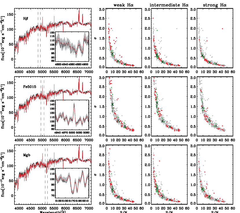
Figure 1.— Error estimation for absorption-line indices. The observed spectrum of a sample galaxy is shown in the left three panels, together with its best gandalf fit (red lines). In each of these panels, the inset shows the SDSS spectrum and our fit in a specific index region (for H$\beta$, Fe5015 and Mgb from top to bottom, respectively, and as indicated by the dashed vertical lines in each main panel), as well as the flux density range of 100 synthetic realizations of this particular spectrum (grey bands) based on the formal SDSS uncertainties on the flux density and our gandalf fit. The right panels show the range (from top to bottom for the same indices as the left) when considering a sample of 405 objects (grey points) with varying quality of spectra, as traced by S/sN, and different strengths of nebular emission, as traced by the H$\alpha$ line. From left to right, the red and green points highlight objects with increasing strength of H$\alpha$ emission, with green points showing objects within specific S/sN ranges, where the median value of the errors on the absorption-line indices and the standard deviations are shown (crosses and vertical lines).

2.5. Errors

Both the pPXF and gandalf returned formal errors for the stellar and gaseous kinematics and the flux values of the fitted emission lines. From MonteCarlo simulations based on synthetic spectra created from our best gandalf fit to a subsample of galaxies in our catalogue and the formal uncertainties of their SDSS spectra, we verified that the formal uncertainties were consistent with the scatter of the parameter estimations obtained from fitting the synthetic spectra. Errors on the line-strength indices for each single object in our database would be more cumbersome to compute. In fact, although the impact of the statistic uncertainties on the flux densities of the SDSS spectra could be easily described in terms of formal errors in the line indices, the knock-on effect of the uncertainties on the stellar kinematics and - most importantly - on the gandalf emission-line fit would require a MonteCarlo simulation in order to be properly estimated. Since this is not viable for nearly 700,000 objects, we decided instead to attach to any given line-index measurement in the objects of our catalogue the typical uncertainty that is measured in spectra showing a similar quality, a similar stellar kinematic broadening and strength of the emission falling in the pseudo-continuum of index passband of the considered index. To derive such typical errors, we selected a large number of SDSS spectra covering a wide range in quality (quantified by the average value of the S/N ratio between the values of the flux density and the statistical SDSS errors on them), of values of the stellar velocity dispersion $\sigma_{\star}$, and - within similar S/N and $\sigma_{\star}$ values - of strength for the emission possibly affecting the line indices (e.g., [Oiii] $\lambda 5007$ for Fe5015). The strength of the emission lines was quantified by the ratio A/rN of the best fitting amplitude A of the considered line and the level of scatter rN in the residuals of the gandalf fit. Based on our best gandalf fit for these objects and the formal SDSS errors on the flux densities, we created a number of synthetic spectra with a slightly different kinematic broadening and nebular emission, as allowed by the formal uncertainties on the pPXF and gandalf parameters, and re-ran our entire analysis on them to obtain new values for the line-indices. By re-matching each of these synthetic spectra and subsequently measuring the line-strength index after subtracting our best model for the nebular emission, we obtained a range of absorption-line strength values and the corresponding 1$\sigma$-errors. The scatter of such synthetic line-index values around the one measured on the original spectra provided us with the typical errors on the line-strength measured in our catalogue. Fig. 1 shows how their values vary as a function of S/N, $\sigma_{\star}$ and - when applicable, the A/N of the contaminating lines. Furthermore, despite the presence of nebular emission, the error budget in the absorption-line indices is chiefly dominated by the quality of the spectra themselves. The formal uncertainties are also provided for the values of both reddening components included in our gandalf fit. The typical errors for absorption-line indices are listed in Tab. 3.

Table 3Typical errors for absorption-line indices

	S/N$\sim 10$			S/N$\sim 20$			S/N$\sim 30$
Name	A/N$<$4	10$<$A/N$<$25	30$<$A/N$<$50	A/N$<$4	10$<$A/N$<$25	30$<$A/N$<$50	A/N$<$4	10$<$A/N$<$25	30$<$A/N$<$50
$\rm{H\delta_{A}}$	1.434$\pm 0.405$	1.046$\pm 0.212$	0.859$\pm 0.139$	0.462$\pm 0.193$	0.574$\pm 0.100$	0.439$\pm 0.017$	0.323$\pm 0.088$	0.332$\pm 0.018$	0.375$\pm 0.036$
$\rm{H\delta_{F}}$	0.960$\pm 0.294$	0.700$\pm 0.158$	0.557$\pm 0.087$	0.400$\pm 0.066$	0.379$\pm 0.051$	0.292$\pm 0.040$	0.247$\pm 0.055$	0.235$\pm 0.018$	0.214$\pm 0.023$
$\rm{CN_{1}}$	0.038$\pm 0.010$	0.031$\pm 0.007$	0.028$\pm 0.005$	0.013$\pm 0.001$	0.018$\pm 0.003$	0.013$\pm 0.001$	0.009$\pm 0.003$	0.010$\pm 0.001$	0.010$\pm 0.001$
$\rm{CN_{2}}$	0.051$\pm 0.013$	0.035$\pm 0.007$	0.030$\pm 0.005$	0.024$\pm 0.006$	0.019$\pm 0.003$	0.015$\pm 0.001$	0.014$\pm 0.003$	0.010$\pm 0.000$	0.012$\pm 0.001$
Ca4227	0.540$\pm 0.149$	0.442$\pm 0.091$	0.382$\pm 0.042$	0.259$\pm 0.049$	0.258$\pm 0.046$	0.193$\pm 0.012$	0.153$\pm 0.022$	0.168$\pm 0.030$	0.152$\pm 0.016$
G4300	1.180$\pm 0.309$	0.905$\pm 0.159$	0.832$\pm 0.125$	0.507$\pm 0.073$	0.494$\pm 0.067$	0.414$\pm 0.065$	0.283$\pm 0.027$	0.305$\pm 0.028$	0.297$\pm 0.030$
$\rm{H\gamma_{A}}$	1.345$\pm 0.395$	1.019$\pm 0.221$	0.899$\pm 0.116$	0.568$\pm 0.082$	0.559$\pm 0.086$	0.468$\pm 0.067$	0.352$\pm 0.045$	0.338$\pm 0.040$	0.435$\pm 0.051$
$\rm{H\gamma_{F}}$	0.866$\pm 0.283$	0.592$\pm 0.114$	0.538$\pm 0.087$	0.356$\pm 0.045$	0.330$\pm 0.045$	0.264$\pm 0.032$	0.214$\pm 0.031$	0.184$\pm 0.009$	0.225$\pm 0.020$
Fe4383	1.454$\pm 0.324$	1.242$\pm 0.220$	1.160$\pm 0.129$	0.599$\pm 0.060$	0.621$\pm 0.107$	0.571$\pm 0.068$	0.417$\pm 0.044$	0.387$\pm 0.014$	0.444$\pm 0.046$
Ca4455	0.655$\pm 0.183$	0.559$\pm 0.088$	0.523$\pm 0.066$	0.315$\pm 0.035$	0.312$\pm 0.037$	0.257$\pm 0.024$	0.181$\pm 0.018$	0.205$\pm 0.026$	0.211$\pm 0.028$
Fe4531	1.048$\pm 0.218$	1.020$\pm 0.176$	0.968$\pm 0.103$	0.493$\pm 0.064$	0.511$\pm 0.081$	0.426$\pm 0.042$	0.316$\pm 0.025$	0.313$\pm 0.003$	0.328$\pm 0.056$
C4668	1.912$\pm 0.295$	1.745$\pm 0.356$	1.742$\pm 0.234$	0.848$\pm 0.068$	0.881$\pm 0.118$	0.758$\pm 0.054$	0.493$\pm 0.048$	0.564$\pm 0.047$	0.578$\pm 0.022$
$\rm{H\beta}$	0.726$\pm 0.133$	0.646$\pm 0.266$	0.623$\pm 0.068$	0.352$\pm 0.027$	0.299$\pm 0.031$	0.283$\pm 0.029$	0.190$\pm 0.009$	0.208$\pm 0.004$	0.232$\pm 0.026$
$\rm{H\beta_{G}}$	0.523$\pm 0.110$	0.460$\pm 0.180$	0.462$\pm 0.049$	0.242$\pm 0.027$	0.238$\pm 0.037$	0.213$\pm 0.021$	0.148$\pm 0.009$	0.140$\pm 0.004$	0.161$\pm 0.012$
Fe4930	0.912$\pm 0.384$	0.885$\pm 0.237$	0.908$\pm 0.105$	0.539$\pm 0.100$	0.534$\pm 0.231$	0.401$\pm 0.049$	0.274$\pm 0.025$	0.315$\pm 0.013$	0.298$\pm 0.012$
$\rm{OIII_{1}}$	0.693$\pm 0.147$	0.743$\pm 0.123$	0.649$\pm 0.127$	0.350$\pm 0.075$	0.402$\pm 0.051$	0.309$\pm 0.109$	0.205$\pm 0.030$	0.244$\pm 0.016$	0.223$\pm 0.010$
$\rm{OIII_{2}}$	0.525$\pm 0.114$	0.604$\pm 0.296$	0.508$\pm 0.300$	0.384$\pm 0.101$	0.281$\pm 0.086$	0.223$\pm 0.218$	0.226$\pm 0.128$	0.278$\pm 0.100$	0.141$\pm 0.043$
Fe5015	1.606$\pm 0.361$	1.668$\pm 0.327$	1.446$\pm 0.310$	0.789$\pm 0.127$	0.767$\pm 0.070$	0.814$\pm 0.105$	0.520$\pm 0.111$	0.483$\pm 0.009$	0.544$\pm 0.066$
$\rm{Mg_{1}}$	0.021$\pm 0.012$	0.020$\pm 0.003$	0.020$\pm 0.005$	0.009$\pm 0.003$	0.010$\pm 0.001$	0.009$\pm 0.003$	0.006$\pm 0.001$	0.006$\pm 0.000$	0.007$\pm 0.001$
$\rm{Mg_{2}}$	0.022$\pm 0.006$	0.022$\pm 0.006$	0.024$\pm 0.006$	0.012$\pm 0.002$	0.015$\pm 0.004$	0.010$\pm 0.002$	0.008$\pm 0.001$	0.007$\pm 0.001$	0.007$\pm 0.001$
$\rm{Mg_{b}}$	0.742$\pm 0.265$	0.816$\pm 0.186$	0.779$\pm 0.048$	0.377$\pm 0.027$	0.406$\pm 0.137$	0.391$\pm 0.067$	0.237$\pm 0.013$	0.243$\pm 0.031$	0.242$\pm 0.015$
Fe5270	0.931$\pm 0.204$	0.904$\pm 0.367$	0.910$\pm 0.141$	0.405$\pm 0.072$	0.447$\pm 0.072$	0.480$\pm 0.125$	0.260$\pm 0.050$	0.275$\pm 0.014$	0.304$\pm 0.018$
$\rm{Fe5270_{S}}$	0.634$\pm 0.154$	0.644$\pm 0.291$	0.665$\pm 0.082$	0.277$\pm 0.048$	0.277$\pm 0.043$	0.318$\pm 0.124$	0.181$\pm 0.038$	0.294$\pm 0.158$	0.204$\pm 0.010$
Fe5335	0.882$\pm 0.288$	0.905$\pm 0.149$	0.817$\pm 0.208$	0.506$\pm 0.068$	0.461$\pm 0.048$	0.390$\pm 0.050$	0.284$\pm 0.050$	0.406$\pm 0.080$	0.318$\pm 0.038$
Fe5406	0.669$\pm 0.252$	0.664$\pm 0.299$	0.734$\pm 0.094$	0.339$\pm 0.072$	0.376$\pm 0.075$	0.284$\pm 0.078$	0.191$\pm 0.023$	0.243$\pm 0.004$	0.267$\pm 0.089$
Fe5709	0.553$\pm 0.152$	0.484$\pm 0.144$	0.539$\pm 0.109$	0.237$\pm 0.013$	0.234$\pm 0.037$	0.216$\pm 0.035$	0.154$\pm 0.030$	0.167$\pm 0.021$	0.183$\pm 0.018$
Fe5782	0.476$\pm 0.102$	0.395$\pm 0.071$	0.463$\pm 0.087$	0.196$\pm 0.080$	0.235$\pm 0.030$	0.175$\pm 0.035$	0.139$\pm 0.006$	0.146$\pm 0.010$	0.131$\pm 0.023$
NaD	0.601$\pm 0.172$	0.530$\pm 0.141$	0.644$\pm 0.112$	0.271$\pm 0.037$	0.353$\pm 0.083$	0.260$\pm 0.037$	0.175$\pm 0.028$	0.225$\pm 0.013$	0.191$\pm 0.032$
$\rm{TiO_{1}}$	0.015$\pm 0.004$	0.015$\pm 0.004$	0.019$\pm 0.005$	0.008$\pm 0.001$	0.008$\pm 0.001$	0.007$\pm 0.001$	0.005$\pm 0.001$	0.005$\pm 0.000$	0.005$\pm 0.001$
$\rm{TiO_{2}}$	0.013$\pm 0.001$	0.013$\pm 0.002$	0.015$\pm 0.003$	0.006$\pm 0.001$	0.007$\pm 0.001$	0.006$\pm 0.001$	0.004$\pm 0.001$	0.004$\pm 0.000$	0.005$\pm 0.000$

2.6. Final Remarks

We conclude this section with a couple of remarks. First, before the strength of the absorption features were assessed at the end of our procedure, the first two steps of our analysis were repeated in order to optimize our gandalf fit. In particular, once the position and the width of the lines were measured the first time, we repeated the pPXF fit by placing a better emission-line mask on only the region where some emission was found. This makes us more confident in the stellar kinematics, in particular for galaxies with little or no emission or in star-forming objects where the Balmer absorption lines are the predominant feature in the stellar spectrum and cannot be properly matched unless the mask around the Balmer emission lines - generally narrower than the absorption lines - is properly adjusted. A better stellar kinematic leads to a better gandalf fit.

A second point to keep in mind is that the second component for the dust extinction used in the gandalf fit - that affecting only the nebular spectrum - should only be considered reliable in the presence of Balmer lines, and thus of an observed Balmer decrement. If no Balmer lines are detected, or if only H$\alpha$ is, then the de-reddened values for the fluxes of all the lines fitted by gandalf will also be very uncertain, and one should only use the observed fluxes. Finally, we stress that even in the presence of a Balmer decrement in a good quality spectrum, the values of the diffuse component for the reddening - approximated as a uniform screen affecting the entire galaxy spectrum - may to some extent be degenerate with the particular gandalf choice for the stellar templates. Determining the star-formation history and the exact values of the reddening in our sample galaxies is beyond the scope of this catalogue, however, and here we are interested mostly in providing the best physically motivated and accurate description of the stellar and nebular spectrum, in order to provide reliable values for the stellar and gas kinematics, for the emission-line fluxes and for the infill-corrected absorption-line indices.

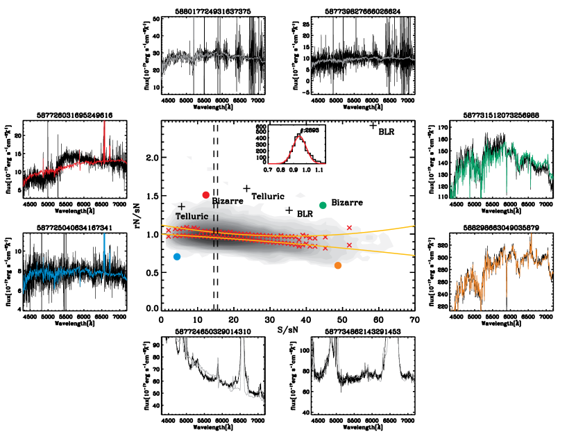
Figure 2.— Quality assessment for continuum with examples inducing bad fits. This figure shows a quality assessment for a continuum region using randomly selected $\sim$46000 objects. Red crosses on the central panel denote the median (lower) and 1 $\sigma$ (upper) distribution for each S/sN bin and orange solid lines fit (note that there is a demarcation line for 1 $\sigma$ in the direction of larger rN/sN.). The vertical dashed lines indicate a specific bin and its Gaussian distribution has been inserted on the top side as an example. The color filled dots correspond to the colored left and right panels and clarify the trend for quality assessments. The black solid lines represent the observed spectra and the coloured lines are the fits. Furthermore, the top and bottom examples with gray fits are the major reasons for the bad fits. These telluric contaminated spectra (top) and Broad Line Regions (bottom) are marked with black crosses on the central panel. A minor reason which brought about bad fits is also denoted by red and green filled dots.

3. Fitting quality assessment

Assessing the quality of our fits to the SDSS spectra is a key to the accuracy of our measurements for the stellar and gaseous kinematics, as well as for the strengths of both the emission and absorption lines. An inadequate model for the observed spectrum, or artificial features in the data themselves is likely to introduce biases to the measured parameters that are not accounted for by our formal errors. Such parameters are affected in different ways by data mismatches. For the stellar kinematics, and in particular for the velocity dispersion, the most crucial match is the stellar continuum across the entire wavelength range, whereas the accuracy of the emission-line parameters (and of the absorption-line indices that are affected by nebular emission) are more sensitive to the quality of the fit in more localized spectral regions around the emission lines.

The quality of the data, as routinely estimated by dividing the average level of the flux density (hereafter S, for signal) by the level of the formal uncertainties for the latter (hereafter sN, for statistical noise), does not guarantee a good fit. Artifacts introduced during data reduction may not be picked up by such an S/sN ratio, whereas a severe template mismatch to the stellar continuum or the presence of additional components in the nebular spectrum (e.g., a Broad Line Region or Wolf-Rayet features that are not included in our standard fitting procedure) may lead to biased results, even in a case of excellent data. A more direct way to assess the quality of our model would be to compare the level of fluctuations in the fit residuals (hereafter rN, for residual noise) to the expected statistical fluctuations, sN. A rN/sN ratio close to unity indicates a good fit, as this ration corresponds to a reduced $\rm{\chi^{2}}$, which is also close to 1.

3.1. Continuum fit

In order to assess the quality of the fit to the stellar continuum and help in isolating biased measurements for the stellar kinematics, we measured the rN/sN ratio in four different wavelength regions of equal width that were devoid of nebular emission. Specifically, we adopted the 4500 – 4700Å, 5400 – 5600Å, 6000 – 6200Å and 6800 – 7000Å wavelength intervals and combined the corresponding values for the rN/sN ratio into a single average, excluding the largest value in order to avoid a spurious contribution of continuum bands, where the SDSS spectra happened to be broken.

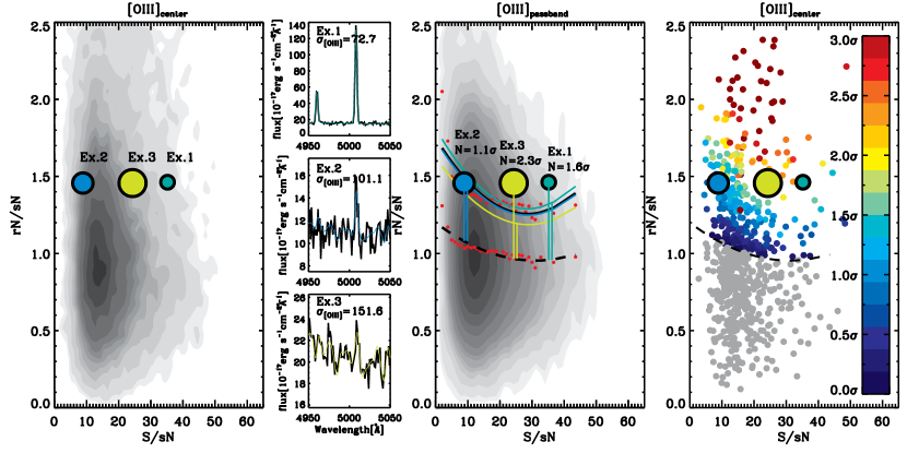
Figure 3.— Quality assessment process for [O iii] $\lambda 5007$ with three examples. Left : The quality assessment plane drawn by a central emission region using randomly selected $\sim$46000 objects. The three examples which have different emission line widths are shown as Ex.1,2 and 3. Middle : Quality assessment plane given by a typical passband. The lower and upper red filled dots are the median and 1$\sigma$ at each S/sN bin. The black dashed and solid lines trace each point. Moreover, [O iii] $\lambda 5007$ emissions for these three examples are shown on left sub-panels in corresponding colors. The black line represents the observed spectrum and the colored one the fit. Once we derived the median and 1$\sigma$ from the typical passband, we measured the N$\sigma$ of every [O iii] $\lambda 5007$ emission. The newly derived 1$\sigma$ are also shown using the same colors. Right : 1,000 objects shown in different colors depend on N$\sigma$. The objects below the median are indicated in gray.

As shown in Fig. 2, for $\sim$46000 randomly selected SDSS galaxy spectra, the distribution of the rN/sN average values for the fit to the stellar continuum as a function of the quality of the spectrum itself, as measured by the S/sN ratio, measured and averaged in the same continuum bands. The vast majority of the spectra were well matched by our model, with rN/sN close to unity. Our ability to match the data also appears to have improved as the quality of the spectra increased. In fact, for data of excellent quality (high S/sN), the level of fluctuation in the fit residual became even smaller than the formal uncertainties in the flux density, suggesting that the latter errors must under-predict the real level of statistical fluctuations in the SDSS spectra in such high-quality regimes.

Fig. 2 also shows a few representative examples of gandalf fits to the the SDSS spectra. As stated above, the quality of the data themselves does not guarantee success or failure in the fit. It is possible to have formally good fits, both in cases of data with good and relatively poor values for the S/sN ratio (orange and blue examples), whereas our model did not necessarily fail only in a case of poor data (red example), but also when the quality was very good (green example).

In general there are three reasons that our objects show rN/sN ratios that are significantly above unity. Most often a poor fit to the continuum is the result of the presence of a conspicuous Broad line region (grey examples, lower panels), which was not noticed by the SDSS pipeline in the process of separating the galaxy from the QSO spectra. Although the presence of broad line regions (BLR) can be accounted for by gandalf (see § 3.3), in the framework of our standard recipe that includes only narrow-line regions, the presence of an additional component leads to a considerable mismatch outside the wavelength regions near the H$\alpha$ and H$\beta$ lines. A second kind of failure occurs for objects in which the adopted stellar library appears to be inadequate in matching the observed SDSS spectrum (dubbed as “Bizarre” in Fig. 2 and already shown in the red and green examples). This occurs in a very small fraction of objects ; however, it often appears the spectra have been contaminated by features in the sky foreground. Finally, for a third kind of spectra, a high rN/sN value is the result of telluric atmospheric features at the red end of the spectra. When such features are present, the SDSS formal errors underestimate the fluctuations around the stellar continuum introduced by the telluric features, biasing the rN/sN value in the 6800-7000 continuum band to high values. We note however, that in this case the fit to the rest of the spectrum is not necessarily poor.

Having ascertained that the vast majority of our models showed good fits for the stellar continuum of the SDSS spectra, we could assign, to any object with rN/sN above unity, a probability of being a true outlier (in the distribution shown in Fig. 2), and hence a galaxy to which the stellar continuum has been poorly matched. For this we determined, as a function of the quality of the spectrum, the median of the rN/sN distribution and corresponding outlier-resistant standard deviation ($\sigma$). We used the rN/sN distributions in S/sN bins containing at least 100 objects (see the inset of the central panel of Fig. 2), which we determined using the Voronoi binning scheme(Cappellari & Copin 2003), and fitted the resulting median and sigma values (red crosses) with a polynomial function (orange lines).

We then computed the distance of each point from the median line in Fig. 2, expressing its distance in units of sigma, N$\sigma$. Since the rN/sN distributions in each S/sN bin were well matched by log-normal functions, such N$\sigma$ value readily gave the probability of a point being a true outlier. For example, N$\sigma$=3 indicated that there was a 99.73% probability that the object was a true outlier and only a 0.27% probability of being the result of random fluctuations.

3.2. Nebular fit

Similar to the case of the stellar continuum, we needed to check the quality of the fit with the emission lines in order determine possible biases in the physical parameters we wanted to measure, such as the line width or fluxes. Even when the nebular emission was clearly detected, it was possible that the underlying assumptions in our modeling approach were not met, due to the presence of a broad line region or to non-Gaussian line profiles, for example.

In order to assess the quality of the emission-line fit using the previous approach, it was important to give as much weight as possible to the deviations that arose only in the spectral regions around the nebular emission, and to adopt, for the wavelength interval where the rN/sN ratio was computed, a width that scaled with the width of the lines. Indeed, if we were to evaluate the rN/sN ratio over a fixed number of sampling elements, at a given fit quality the deviations from the fits of lines of very different widths would contribute unevenly to the rN/sN budget, thus limiting our ability to spot bad fits in the case of narrow lines. For each emission line we thus computed rN/sN around the line within a passband of width equal to five times the gas velocity dispersion $\sigma_{\rm gas}$. To then assess the quality of an emission-line fit in a given object, we normalized the distance from the median line in the rN/sN vs. S/sN diagram using the $\sigma_{\rm rN/sN}$ value (at a given S/sN) that would be found if all of the rN/sN and S/sN ratios had been measured with passbands of identical widths corresponding to the value of the $\sigma_{\rm gas}$ observed in the object of interest. Such a $\sigma_{\rm rN/sN}$ was found by simply rescaling the $\sigma_{\rm rN/sN}$ values obtained using a fixed bandwidth, corresponding, for instance, to the typical value of $\sigma_{\rm gas}$ found in the SDSS galaxies ($\sim 90$ ${\rm km}~{}{\rm s}^{-1}$). For a good fit, the amplitude of the fluctuations around the median value for the rN/sN ratio (at a given data quality or S/sN value) scaled simply with the square root of the number of sampling elements used in computing the rN/sN ratio.

There was a second complication in assessing the quality of the emission-line fit. Even for systems with similar line widths, evaluating the amplitude of the statistical fluctuations in the rN/sN ratio at a given data quality was difficult due to the presence of a larger fraction of formally bad fits compared to the case of the stellar continuum. Put another way, it was more difficult to isolate the tail of the outliers when estimating the standard deviation in the rN/sN histograms for the emission-line fit. To circumvent this problem, for every line that we wanted to check in terms of the quality of our fit, we defined a continuum passband in its immediate vicinity and used the rN/sN vs. S/sN distribution for this passband to determine the reference rN/sN median and sigma profiles that were actually used to assess the quality of each fit. As previously mentioned, such profiles were derived by adopting for the continuum passband a single width, which was set to five times the typical $\sigma_{\rm gas}$ value in the SDSS galaxies, or approximately 90${\rm km}~{}{\rm s}^{-1}$.

Fig. 3 illustrates how this procedure works for the specific case of the [O iii] $\lambda 5007$ emission line. The left panel shows, for the same $\sim$46000 galaxies shown in Fig. 2, the rN/sN vs. S/sN distribution for the [O iii] $\lambda 5007$ fit, adopting for each object a bandwidth equal to five times $\sigma_{[\mbox{O{\sc iii}}]}$. In this panel, we show the positions of three objects with similar values of the rN/sN ratio around the [O iii] $\lambda 5007$ line, but with different $\sigma_{[\mbox{O{\sc iii}}]}$ values, as indicated by the size of the symbols.

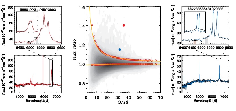
Figure 4.— Broad line region objects. The central panel shows how we picked out broad line regions from the entire DR7 galaxies. The median and 3$\sigma$ distributions are shown with red crosses and orange lines, which are shown on left and right panels. Left : The black and red lines represent the observed spectrum and fit, respectively. The two shaded regions on the top panel are the continuum and blue-side wing of the broadened emission region that was used to derive the flux ratio. The dashed horizontal bars represent the mean flux levels for the specifically defined continuum and wing. The inserted panel on the top is the fitting result, without the new prescription for the broad line region objects. Once we picked the broad line region objects from the entire DR7 galaxies, we re-fitted them to improve the fit. Right : The blue line is our fit.

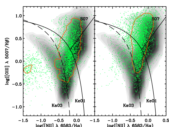
Figure 5.— BPT diagnostic diagram including broad line regions. The objects morphologically classified into early type galaxies by FracDeV and the concentration index were drawn with filled contours. We determined the broad line regions from the “galaxies” in the SDSS DR7, which is shown in green dots in both panels. Many of the green dots moved to Seyfert regimes at the right panel, by applying a new prescription which masked the entire Balmer absorption series to a properly find continuum. Broad line regions, with the exception of widely broadened emission lines, need this new prescription to exactly fit their continuum.

If the median and $\sigma_{\rm rN/sN}$ profiles could be drawn in this panel and used to assess the quality of the [O iii] $\lambda 5007$ fit in these objects, we would have been led to believe that the goodness of the emission-line fit degrades as we move from left to right, to higher S/sN values. This is not quite the case, as illustrated by the central panel. This panel shows the rN/sN vs. S/sN distribution obtained in the continuum passband adjacent to the [O iii] $\lambda 5007$ line, centered at 5006.7Å and adopting a width equal to five times 90${\rm km}~{}{\rm s}^{-1}$. The dashed and solid black lines show the median rN/sN values and the level where the objects are one $\sigma_{\rm rN/sN}$ away from the median, respectively (using the same method as for the continuum fit). For lines that are considerably broader than 90${\rm km}~{}{\rm s}^{-1}$ the statistical fluctuations around the median ought to be considerably smaller since a broader passband containing a larger number of sampling elements was adopted. Conversely, the quality of the fit for much narrower lines should be compared against a higher bar. This is illustrated by the coloured solid lines in the central panel of Fig. 3, which shows the level where objects with the same $\sigma_{[\mbox{O{\sc iii}}]}$ of the three considered examples should lie when found one $\sigma_{\rm rN/sN}$ away from the median rN/sN line. When such yardsticks are used to express the distance from the median in terms of $N_{\sigma}$ values, although the object with highest S/sN ratio (green point) lies further away from the median line, due to its narrower [O iii] $\lambda 5007$ line, the quality of its gandalf fit was not much worse than in the case of the galaxy with the worse data (lowest S/sN, light blue) and was much better than for the object with the broadest [O iii] $\lambda 5007$ lines (light green). Using this quality-assessment scheme, the right-hand panel shows how the goodness of our emission-line fit can be illustrated (albeit only for a small number of objects for the sake of clarity), by colour-coding each point in the rN/sN vs. S/sN diagram for the [O iii] $\lambda 5007$ line according to the $N_{\sigma}$ values derived in the rN/sN vs. S/sN diagram for the continuum band adjacent to [O iii] $\lambda 5007$.

Typically, formally bad emission-line fits occur either in the presence of strong lines where even small deviations from a Gaussian profiles lead to high rN/sN values, or in the presence of an additional BLR component. Non-Gaussian lines can have a double-horned shape. For instance, in the case of the Balmer lines, tracing star-formation activity confined to a circumnuclear ring can show blue or red wings, presumably due to out or inflows of gaseous material, or, can display the triangular Voigt profile that is typical of strong AGN activity. Our Gaussian fit could lead to biased measurements for the position of the lines with blue or red wings, and to an overestimation of the width of the true thermal component in lines with a Voigt profile. Our flux estimates, on the other hand, are not heavily affected by the presence of non-Gaussians profiles. This is not the case, however, for objects with an additional BLR component, in particular when gandalf chooses to match the broad lines rather than the narrow component of the Balmer spectrum. Since the BLR fluxes can greatly exceed the flux of the narrow Balmer lines, when these objects are plotted on standard BPT diagrams, such as the [N ii] $\lambda 6584$/H$\alpha$ vs. [O iii] $\lambda 5007$/H$\beta$ diagram, they can be easily spotted in regions with very low values for the [N ii] $\lambda 6584$/H$\alpha$ or [O iii] $\lambda 5007$/H$\beta$ ratio that are not occupied by other galaxies with well-matched nebular spectra from AGNs or star-forming regions (refer to the following section). Conversely, no object with a non-Gaussian profile ends up in similarly strange regions of the BPT diagrams.

3.3. Broad Line Region

In the previous two subsections, we argued that the presence of a broad-line region frequently causes a bad fit to both the emission lines and the stellar continuum, in particular near the H$\alpha$ and H$\beta$ lines. Yet, provided that the presence of a BLR is automatically spotted, the impact of such a component on the pPXF extraction of the stellar kinematics and the subsequent gandalf fit to both the stellar continuum and nebular lines can be easily dealt with. In fact, one needs only to add a second series of broader Balmer lines in the gandalf setup to place a broader mask around to Balmer lines during the pPXF fit and then include the BLR component in the gandalf fit.

In order to recognize the presence of BLR, we looked for a “shoulder” in the continuum region adjacent to the H$\alpha$+[N ii] $\lambda 6584$ region, which would otherwise be relatively flat. For this, we computed the ratio between the flux levels observed in two spectral regions of equal width on the blue side of the H$\alpha$+[N ii] $\lambda 6584$ blend. The first was placed as close as possible to the [N ii] $\lambda 6548$ (avoiding any flux from this line even for the broadest narrow-line region, $\sim 300$${\rm km}~{}{\rm s}^{-1}$), and the second was located just beyond the extent of the broadest BLR (centering it on the blue side of the 6594Å absorption line that is predominantly due to Calcium and Iron). Then, similar to our quality-assessment procedures, once such flux ratio was measured in a given object, we simply checked to determine if it was exceptionally high compared to the distribution of other flux ratios in spectra of similar quality. Fig. 4 shows two examples of spectra with BLR components and how our procedure isolated them. This diagram juxtaposes the quality of the spectra in the H$\alpha$+[N ii] $\lambda 6584$ region (using the S/sN ratio in the 6000 – 6200Å window, § 4.1) and the flux ratio defined above. This figure also shows the gandalf fit according to our standard prescription and, after adding a BLR component, and illustrates how our standard gandalf fit does not always fail while choosing to match the BLR region (as already noticed in § 4.2).

To assess the efficiency of our criterion in spotting BLR components, we visually inspected the spectra and the residuals of the standard gandalf fit for 10,000 randomly chosen objects, labeling those where we recognized the presence of a BLR. Adopting a 3$\sigma$ cut to isolate exceptionally high values for the previously defined flux ratio, our procedure selected 83% of the BLR that we identified by eye, while wrongly deeming likely the presence of a BLR in 0.8% of the objects where we had found none. Although these figures are quite encouraging, it must be acknowledged that only the strongest BLR regions can be identified if the S/sN is small(i.e., poor-quality spectra).

Even then, such BLR components appear in a non-negligible fraction of the SDSS spectra of nearby galaxies, as overall we found 8,610 objects with a BLR component out or the entire DR7 sample, or almost 1.3% of the galaxies.

As mentioned in § 4.2, the impact of a failed gandalf fit due to a BLR can be crucial when classifying the nebular emission with standard BPT diagrams. In fact, when the gandalf algorithm opts to fit the BLR region within our standard prescription, the object will move to a strange region in the BPT diagram, below and to the left of the area occupied by the star-bursting systems. Adding a BLR component in the gandalf fit rectifies this problem, and usually moves the narrow-line components of these galaxies back to the regions of the BPT diagram that are occupied by active galactic nuclei, either Seyfert nuclei or low-ionization nuclear emission regions (LINERs). Such a correction was particularly evident when considering a sample of objects that rarely showed signs of central star formation, such as early-type galaxies. Fig. 5 shows an area occupied by the early-type galaxies in our DR7 sample (as morphologically classified in § 7.2) in the standard [N ii] $\lambda 6584$/H$\alpha$ vs. [O iii] $\lambda 5007$/H$\beta$ diagnostic diagram, as well as the position of those objects where we spotted the presence of BLR, before and after adding a BLR component in the gandalf fit, in the left and right panels, respectively. For the vast majority of the objects with a BLR, our procedure failed to match the narrow H$\alpha$+[N ii] $\lambda 6584$ lines in the standard gandalf fit and they resided in the lower left side of the BPT diagram. If we properly dealt with the BLR component, however, they generally moved to the region occupied by Seyfert nuclei.

4. Database

Our measurements of the stellar and nebular kinematics, for the strength of both the emission lines and the stellar absorption features, for the diffuse and nebular reddening components, as well as our assessments of the quality of the fit to the stellar continuum and each of the emission lines, formed a rather complicated database. To facilitate distribution, we decided to organize our pPXF, gandalf and absorption-line index measurements in IDL structures, which allowed us to group all the emission- and absorption-line quantities. Such structures were then saved in single FITS files for each of the objects in our public catalogue. These files can be queried for single or multiple objects by their SDSS ID, galaxy coordinate and redshift via a web interface, or can be downloaded in single archive. For the case of single objects, we also provide a second FITS file showing the gandalf fit to the object of interest.

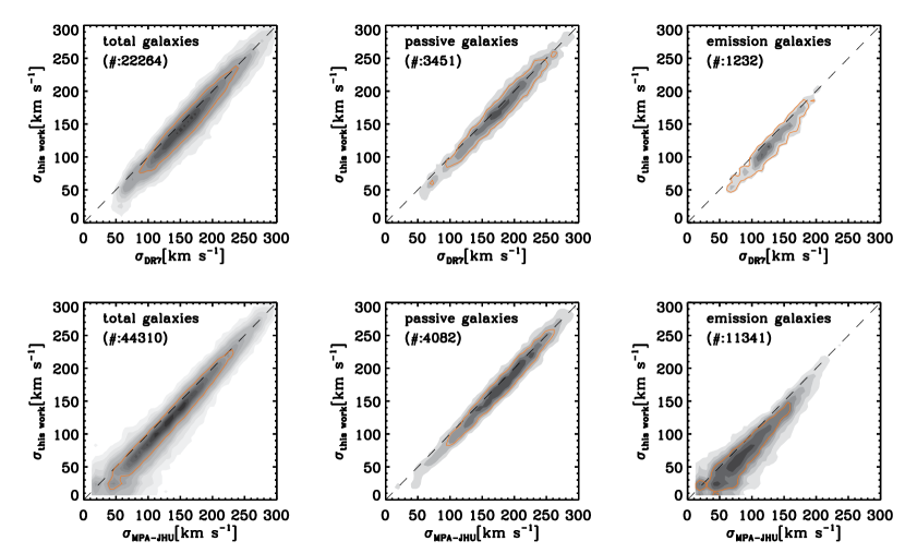
Figure 6.— Comparison between our values for the central stellar velocity dispersion and those computed by the SDSS pipeline (upper panels) and those listed in the MPA-JHU catalogue (lower panels). Starting from an original sample of randomly drawn 46,000 objects from our catalogue, the left panels shows the comparisons with matches in the SDSS and MPA-JHU databases, whereas the central and left panels shows objects with no nebular emission (A/N$<1$ for [O iii] $\lambda 5007$, H$\alpha$ and [N ii] $\lambda 6584$) or with strong lines (A/N$>4$ for the same lines, at the same time), respectively. In each panel the dashed lines show the one-to-one line and the solid lines show the 1$\sigma$ contour for the plotted data.

The output parameters in the IDL structures are organized following the logical order of our fitting procedure. First we found the pPXF outputs, the stellar redshift $z_{\star}$ and velocity dispersion $\sigma_{\star}$ (in ${\rm km}~{}{\rm s}^{-1}$). These are followed by the nominal quality of the spectra and of our fit in the continuum, as quantified by the S/sN and rN/sN ratios introduced in §4.1, which relate to the probability that the fit is biased by some artificial or unaccounted feature, as given by the N_σ parameter. Negative N_σ values occur when the rN/sN ratio are below the median value, and always indicate a good fit. Next are the gandalf emission-line measurements, which we provide for all of the lines listed in Tab.1, in addition to the H$\beta$ line. For each line we list the observed and de-reddened fluxes (in $\rm 10^{-17}erg\,s^{-1}\,cm^{-2}\,\AA^{-1}$), the equivalent width of the line (in negative Å values), the A/N ratio that relates to how well a line is detected (§ 2.2), and the N_σ value (as defined in a §4.2). The strength of the lines and our ability to match them is then followed by the redshift and width of the recombination and forbidden lines (labelled as $z_{\rm H\alpha}$, $\sigma_{\rm H\alpha}$, $z_{\rm[O\,{\sc III}]}$, $\sigma_{\rm[O\,{\sc III}]}$) as well as by the value of the interstellar reddening $A_{V}$, which includes a second, nebular component $A_{V,neb}$, when the Balmer decrement is detected (§ 2.2). The presence of a BLR is also flagged at this point. Although no detection cut based on the A/N values was applied to the emission-line measurements, these should be deemed unreliable when little or no emission is detected. Last, but not least, are the absorption-line measurements for each of the indices listed in Tab. 2, measured in Å. It is most likely that only the objects with SDSS of the best quality (e.g., $\rm S/sN\geq 30$) would prove useful.

All the previously listed redshift, velocity dispersion, flux, equivalent width and reddening values are also accompanied by their corresponding formal uncertainties. In some cases, due to the presence of sky lines or gaps and artifacts in the SDSS spectra, the values of the parameters can diverge, in which case they are flagged.

We provide our entire database (line strengths, quality assessments, fitting SED) at http://gem.yonsei.ac.kr/ossy/.

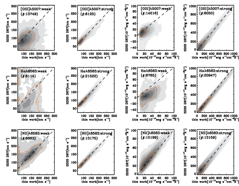
Figure 7.— Comparison between our values for the emission-line width and flux and those from the SDSS pipeline, starting from the same 46,000 randomly drawn objects used for Fig. 6. From top to bottom we compared the measurements for the [O iii] $\lambda 5007$, H$\alpha$ and [N ii] $\lambda 6584$ lines, for the line widths (in the left panels) and the line fluxes (in the right ones). The left and right panels are further split according to the global strength of the emission (weak : 2$<$A/N$<$5 for [O iii] $\lambda 5007$, H$\alpha$ and [N ii] $\lambda 6584$, strong : A/N$>$10 for the same lines, at the same time). In each panel, the dashed line shows the one-to-one line and the solid contour shows the 1$\sigma$ contour level for the plotted data.

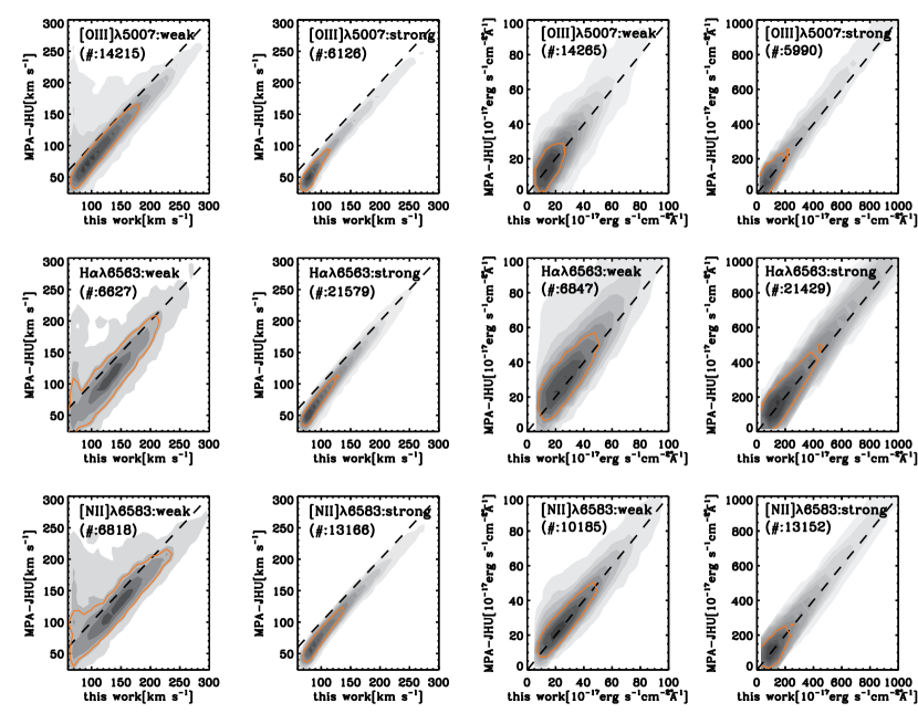
Figure 8.— Same as Fig. 7, but showing a comparison between the MPA-JHU values and those reported in this work.

5. Comparisons with other public database

There are two existing databases of SDSS DR7 data with which we can compare our own measurements. The first consists of the SDSS DR7 pipeline outputs, and the second comes from the MPA-JHU release of DR7 spectral measurements. As in previous releases, the SDSS DR7 pipeline does not remove the nebular emission prior to the absorption-line measurements, so we expected biases in cases of considerable ionised-gas emission. On the other hand, by following the method of Tremonti et al. (2004), the MPA-JHU measurements were based on a procedure that is similar to ours, whereby the nebular contribution to the spectra and the corresponding absorption-line infill was carefully treated. Yet, from the description of the MPA-JHU database, we determined some technical differences between their procedure and the method adopted here which proved important for interpreting possible discrepancies with our measurements. For instance, we measured the emission-line fluxes while simultaneously matching the stellar continuum and the nebular emission with gandalf, whereas the MPA-JHU emission-line measurements were carried out on the residuals of a previous fit to the stellar continuum, presumably while masking the regions affected by emission, which we did when extracting the stellar kinematics with pPXF.

5.1. Stellar Kinematics

With the data in Fig. 6, we began by comparing, for the same subsample of randomly drawn $\sim$46000 objects used in Fig. 2 and Fig. 3, our pPXF velocity dispersion $\sigma_{\star}$ measurements with the corresponding values from both the SDSS DR7 and MPA-JHU databases. The overall agreement between the various measurements was good, although our $\sigma_{\star}$ values appeared to follow more closely the SDSS DR7 data than the MPA-JHU. This occurred, in particular, at the low-$\sigma_{\star}$ regime, which is inhabited mostly by relatively faint spiral galaxies showing considerable amounts of nebular emission. In fact, at the very low $\sigma_{\star}$ end of our sample the presence of emission caused most of the SDSS DR7 measurements to fail, and whereas the MPA-JHU catalogue reports $\sigma_{\star}$ values for these objects, in most cases their values exceed ours. The large scatter in this regime can be explained by considering the low S/sN ratio of the spectra for such faint spirals, but such a bias cannot be easily explained. It is worthy of note, however, that based on simulations similar to those presented in § 2.5, and featuring SDSS spectra for both very old and young stellar populations, we found the pPXF can recover $\sigma_{\star}$ values that scatter evenly around the input values down to $\sigma_{\star}=50$${\rm km}~{}{\rm s}^{-1}$ and S/sN = 10.

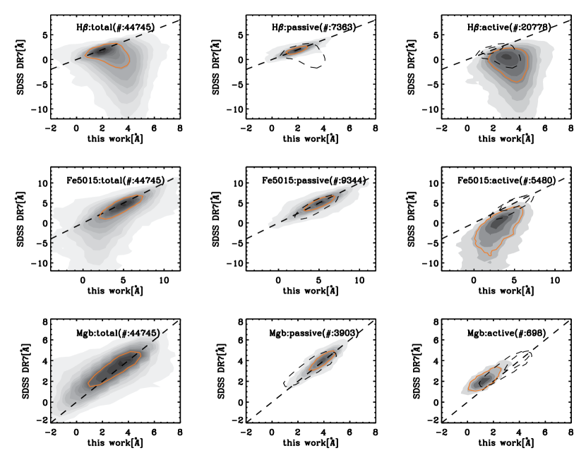
Figure 9.— Comparison between our values of the H$\beta$, Fe5015 and Mgb indices (top, middle, lower panels) and those from the SDSS pipeline, starting from the same 46,000 randomly drawn objects used for Fig. 6. As in Fig. 6, the left panels show all of the objects present in both databases, whereas the central and right panels show only the objects with weak nebular emission or with strong emission-lines. For the H$\beta$ and Fe5015 indices, we defined weak objects as those with A/N values below 1 for the H$\alpha$ and [O iii] $\lambda 5007$ lines, and active objects as those with A/N$>10$ for those lines. In the case of Mgb, we required intermediate A/N values for H$\alpha$, [O iii] $\lambda 5007$ and the [N i] $\lambda\lambda 5198,5200$ lines simultaneously to pick objects with weak emission. Conversely, we required strong emission in all three lines in order to select objects where the [N i] $\lambda\lambda 5198,5200$ contamination to the Mgb index was important. In each panel the dashed line shows the one-to-one line and the solid contour shows the 1$\sigma$ contour level for the plotted data, as in Fig. 6, in this figure the dashed lines also show the contours plotted in the previous panels (from left to right).

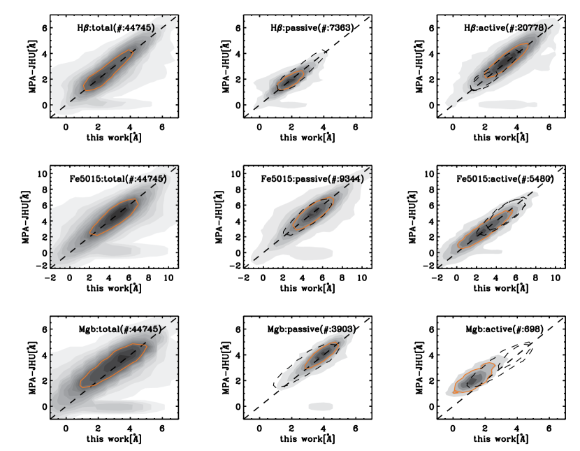
Figure 10.— Same as Fig. 9 but showing a comparison between the MPA-JHU values and those reported in this work.

5.2. Nebular Emission Fit

Continuing with the nebular fit, Fig. 7 and Fig. 8 show how our values for the width and the flux of strong lines such as [O iii] $\lambda 5007$, H$\alpha$ and [N ii] $\lambda 6584$ compare against the same quantities from the DR7 pipeline and the MPA-JHU catalog, respectively. When comparing our values to the DR7 and MPA-JHU measurements, we used observed and intrinsic line-widths, respectively, and in both cases the flux values that were still affected by reddening due to dust in the SDSS objects. We further corrected the DR7 fluxes for foreground galactic extinction to bring them in line with our and the MPA-JHU measurements, and brought the MPA-JHU fluxes back to their original values before the renormalisation for extended sources.

Our line-width and flux measurements agreed fairly well with the DR7 measurements (Fig. 7), in particular when the lines were strong and thus the manner by which the stellar continuum was accounted for should have had only a very limited impact on the emission-line width and flux estimation based on the Gaussian fits. Still, even at these regimes our H$\alpha$ flux values appear to exceed the DR7 measurements by a few percent. Furthermore, as we consider weaker lines, the way the H$\alpha$ flux measurements compared to each other appeared to be systematically biased, rather than being simply affected by a larger scatter due to larger relative errors on the measurements of weak lines in both the DR7 and our dataset, as seems to be the case for [O iii] $\lambda 5007$ and [N ii] $\lambda 6584$. Our flux values became systematically larger than the DR7 measurements as the H$\alpha$ lines become weaker, which is to be expected given that we accounted for the presence of the underlying stellar spectrum and that in this regime the strength of the H$\alpha$ emission became comparable to its corresponding stellar absorption feature.

No such bias as a function of the emission-line strength was observed when we compared our H$\alpha$ flux values with the MPA-JHU measurements, which do account for the stellar continuum (Fig. 8), although our intrinsic H$\alpha$ line-width values were larger than the MPA-JHU estimates. From the limited information provided with the MPA-JHU on-line catalog, it is difficult to understand the cause of such small deviations; however, in the strong-emission regime where the flux estimates should be consistent between all three databases, our values were in agreement with the DR7 values, whereas the MPA-JHU measurements were not.

5.3. Absorption Line Measurements

We conclude this section by presenting Fig. 9 and Fig. 10, where we compare our line-strength measurements with the values for the same Lick indices provided by both the DR7 pipeline and the MPA-JHU catalogue. The DR7 release webpages specify that the DR7 measurements were made on the original SDSS spectra, without degrading their resolution to match the resolution of the Lick/IDS system. Furthermore, a first inspection of the objects with good quality spectra and that were completely devoid of emission revealed that this was also the case for the MPA-JHU measurements and that in both cases no attempt was made to correct the line-strength measurements for the impact of kinematic broadening. The central panels of Fig. 9 and Fig. 10 show how, for passive objects, our uncorrected measurements were well-matched with both catalogues.

When objects with emission are considered, however, the DR7 values (Fig. 9) were heavily biased for the Lick indices where an emission line could fall either in the index passband or within the adjacent regions that were used to estimate the level of the pseudo-continuum above the absorption line region. In fact, during the DR7 pipeline analysis, the nebular emission was not subtracted prior to the line-strength measurements. When the emission-line fell within the index passband, as happened for the H$\beta$ and [Oiii] $\lambda 5007$ lines in the case of the H$\beta$ and Fe5015 indices (top and central panels of Fig. 9 and Fig. 10), the strength of the absorption line was under-estimated. When the emission fell in one of the continuum passbands, as happened for the [N i] $\lambda\lambda 5198,5200$ doublet in the case of the Mgb index (lower panels), the line-strength was over-estimated, as it was measured against an artificially enhanced pseudo-continuum level (see also Emsellem, Goudfrooij, & Ferruit 2003). On the other hand, the MPA-JHU line-strength measurements tended to agree with ours in the presence of nebular emission, as they were also corrected for line-infill (Fig. 10, top and middle panels for H$\beta$ and Fe5015). Yet, the MPA-JHU catalogue does not include several of the emission lines that are present in our catalogue, such as the [N i] $\lambda\lambda 5198,5200$ doublet, which explains why disagreement between the Mgb measurements still persists (Fig. 10 (lower panels)).

As a final remark, it should be noted that the necessary correction for the impact of kinematic broadening can be quite severe in the most massive galaxies with correspondingly high values for the central stellar velocity dispersion (Kuntschner 2004). This occurs, in particular, for the case of indices, such as Fe5015 and Mgb, that were typically used to estimate the metallicity of the degree of $\alpha$-enhancement of stellar populations, for which not accounting for kinematic broadening would lead to an underestimation of their values. When we considered that the MPA-JHU measurements for the Mgb index could have been over-estimated in the presence of [N i] $\lambda\lambda 5198,5200$ emission, we note that using the MPA-JHU values could lead to over-estimated values of the Mgb/Fe5015 ratio, which is a useful gauge of $\alpha$-enhancement (Worthey, Faber, & Gonzalez 1992).

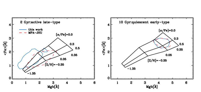
Figure 11.— Effect of [N i] $\lambda\lambda 5198,5200$ emission on the Mgb absorption-line index and connected estimates of the $\alpha$-element abundance. The left panel shows a comparison of the position of a sample of spiral galaxies with strong nebular emission (shown by the 1$\sigma$ contour level of the data) in the Mgb vs. $<$Fe$>$ diagram with the model grids of Thomas et al. (2003). The solid and dashed contours indicate the distribution of the data from our catalogue and from that of the MPA-JHU database. Similarly, the right panel shows the same quantities, but for a sample of quiescent early-type galaxies (see § 5.3.1 for more detail). The model grids assume a luminosity-weighted mean age of 2 Gyr and 10 Gyr for the spirals and early-type galaxies, respectively.

5.3.1 The impact of the [N i] $\lambda\lambda 5198,5200$ doublet on element abundance estimates

To give an example of the potential extent of this problem, we considered two different subsamples: one comprising spiral galaxies displaying nebular emission, and a second including only quiescent early-type galaxies. These objects were morphologically selected as described in the following section and, after applying our standard $A/N>4$ and $A/N<1$ requirement for strong lines in order to pick active and quiescent objects (in addition to requiring the detection or not of [N i] $\lambda\lambda 5198,5200$ emission), we assembled 311 and 579 objects for spirals and early-type galaxies, respectively. Adopting an indicative luminosity-weighted age of 2 and 10 Gyr for the stellar populations of these two classes of galaxies, we compared the position of ours and the MPA-JHU measurements for the Iron and Magnesium sensitive $<$Fe$>$ and Mgb indices to the grids of Thomas et al. (2003) to determine stellar population models of varying metallicities and overabundance of $\alpha$ elements, such as Magnesium(Fig. 11). For the case of passive objects (right panel), the 1-$\sigma$ contours for the distribution of ours and the MPA-JHU measurements overlapped well and indicated an $\alpha$ enhancement with respect to the solar values of the $[\alpha/{\rm Fe}]$ ratio. On the other hand, for the case of spirals (left panel), not accounting for the presence of the [N i] $\lambda\lambda 5198,5200$ lines led to an overestimation of the Mgb/$<$Fe$>$ ratio, and therefore an abundance of $\alpha$ elements in the central regions of spiral galaxies which, from our database, would seem to have solar abundances.

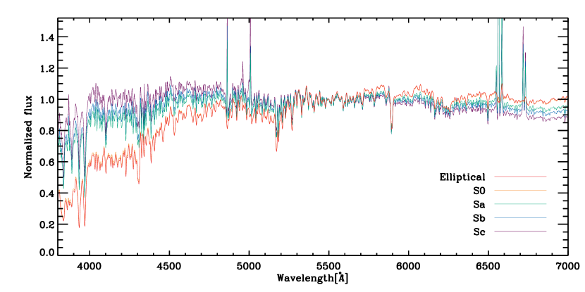
Figure 12.— Stacked galaxy templates for the various morphological types listed in Tab. 4 (except edge-on late-type spirals), normalized at 5,500 Å.

6. Galaxy spectral templates

Large-scale spectroscopic surveys, such as SDSS, have made it possible to create spectral templates for galaxies of various kinds and morphological classes, which can be used as inputs in SED fitting routines where optical template spectra are needed, such as in photometric redshift codes (e.g. Stebbins & Whitford 1948; Baum, W. A. 1962; Bolzonella, Miralles & Pello 2000; Wolf et al. 2004). Therefore, we present here template spectra of elliptical, S0, Sa, Sb, Sc, and edge-on late-type galaxies, in the wavelength range between 3,799Å and 7,000Å(see Figs. 12, 13 and 14).

We began the construction of our stacked galaxy spectra by restricting ourselves to a volume-limited parent sample of objects with $M_{r}$ $<$ -17.62 and in the narrow redshift range of 0.020 $<$ z $<$ 0.025. This ensured a sufficient quality for the spectra to enable analysis and stacking, and to ensure that galaxy evolution would not be a concern given than such a redshift slide covers only $\sim$ 67 Myr.

Table 4The properties of the sample galaxies used for the SED stacking

Morphology	N	${\texttt{FracDeV}}_{g}$	${\texttt{FracDeV}}_{r}$	${\texttt{FracDeV}}_{i}$	$C_{r}$	$isoB_{r}$/$isoA_{r}$	$isoA_{r}$	$R_{\rm eff,r}$	$Fraction_{r}$
Elliptical	111	1.0$\pm$0.0	1.0$\pm$0.0	1.0$\pm$0.0	3.3$\pm$0.2	0.8$\pm$0.1	69.1$\pm$19.9	5.9$\pm$1.8	17.1$\pm$4.2
S0	85	1.0$\pm$0.0	1.0$\pm$0.0	1.0$\pm$0.0	3.3$\pm$0.1	0.7$\pm$0.1	68.4$\pm$17.1	5.6$\pm$1.5	19.7$\pm$4.6
edge-on late-type	175	0.0$\pm$0.0	0.0$\pm$0.0	0.0$\pm$0.0	2.4$\pm$0.1	0.2$\pm$0.0	61.1$\pm$18.7	23.7$\pm$5.2	8.7$\pm$2.6
Sa	28	0.0$\pm$0.0	0.0$\pm$0.0	0.0$\pm$0.0	2.0$\pm$0.1	0.6$\pm$0.2	57.6$\pm$13.4	25.2$\pm$4.9	4.6$\pm$1.7
Sb	32	0.0$\pm$0.0	0.0$\pm$0.0	0.0$\pm$0.0	2.0$\pm$0.2	0.6$\pm$0.2	60.0$\pm$16.9	26.9$\pm$4.2	4.9$\pm$2.6
Sc	21	0.0$\pm$0.0	0.0$\pm$0.0	0.0$\pm$0.0	1.9$\pm$0.2	0.7$\pm$0.2	50.7$\pm$8.2	25.5$\pm$4.3	4.5$\pm$1.2

We then applied a set of selection criteria based on SDSS estimates for the galaxy size, inclination and light concentration in order to obtain early- and late-type galaxies for which we could check the morphology by eye. To allow such a visual inspection, we restricted ourselves to sufficiently extended and face-on SDSS galaxies, by imposing a lower limit on the angular size as $isoA_{r}>40^{\prime\prime}$ and the axis ratio as $isoB_{r}/isoA_{r}>0.4$. Furthermore, we initially split early-type galaxies from their late-type counterparts by looking for objects with concentrated light profiles that were best matched by a de Vaucouleur profile. For this we required values for the FracDeV parameter, which measures how well the light profile is matched by a de Vaucouleur law rather than by an exponential profile, above 0.95 (see also Schawinski et al. 2007) and values for the concentration index $C_{r}$ ($C_{r}=r_{90}$/$r_{50}$ where $r_{90}$ and $r_{50}$ are the radii containing 90 and 50% of the light, respectively) above 2.6 (see also Shimasaku et al. 2001; Strateva et al. 2001).

Through this pre-selection we obtained 2591 galaxies, which were all carefully inspected by eye and which in the end yielded 452 objects, subdivided in E, S0, Sa, Sb and Sc morphologies (as listed in Tab. 4). This included 175 late-type and edge-on galaxies as well, which were selected in a similar way, but by imposing $isoB_{r}/isoA_{r}<0.3$. Our selection criteria is summarized in Tab. 4.

With these robustly classified objects at hand, we proceeded to combine their SDSS central spectra by stacking the best gandalf spectral fit for each of them, once each of our models was brought back to the rest frame and normalized in flux at 5,500Å. In this process we also recorded, at each wavelength, the 1$\sigma$ scatter of the flux values contributed by each of the stacked spectra, in order to estimate how much the spectral energy distributions of the galaxies entering our templates differed from each other. Fig. 12 presents all such spectral templates (except for the edge-on late-type spirals), which extend from 3,799Å to 7,000Å, and Figs 13 and 14 show each of the spectral templates by itself, together with SDSS images for the twelve sample galaxies in each morphological class that we selected.

As a concluding remark, we note that our stacked spectra encompass only the central regions of the objects we selected. Specifically, on average the $3^{\prime\prime}$-wide SDSS fibers sample 20% of the light from the E and S0 galaxies in our sample, and 5% for the late-type galaxies. For our E, S0, Sa, Sb, and Sc galaxies, the difference between their total magnitudes and their fiber magnitudes is 0.02, 0.01, 0.09, 0.12 and 0.07 mag, respectively. Obviously, our templates are more representative for early-types than for late-type. Even for late-types, the systematic trend along the morphological type is still visible in our templates, and the systematic offset from the total light properties is only of order 10%.

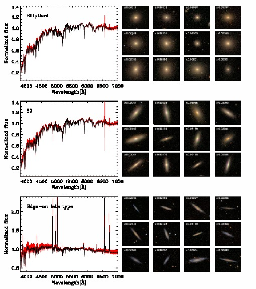
Figure 13.— Stacked templates and optical images for elliptical, lenticular and edge-on late-type galaxy morphologies. The left panel includes the 1$\sigma$ scatter estimated while stacking the spectra, with the aim of conveying how much difference there was in the shape of the spectral energy distribution of the galaxies used in each morphological template. As in Fig. 12, the templates were normalized at 5,500 Å. Each image is 100.0″$\times$ 100.0″ across, corresponding, on average, to a physical size of 100 kpc.

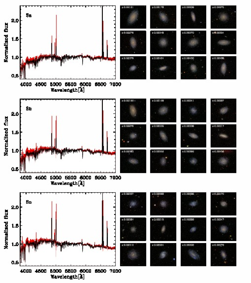
Figure 14.— Same as Fig. 13, but for Sa, Sb and Sc morphologies.

7. Summary

We presented a new database of absorption and emission-line measurements for all galaxies within a redshift of 0.2, for which there are central spectra in 7^th SDSS data release. We modeled the stellar and nebular components of such SDSS spectra, adopting publicly available IDL machineries, with the aim of extracting both reliable and reproduceable measurements for the stellar velocity dispersion, the strength of various absorption-line features, and for both the flux and width of the recombination and forbidden emission lines that were observed in the central region of our sample galaxies. In an attempt to improve on existing databases of SDSS spectral measurements, we included in our fit to the stellar continuum both standard stellar population models and empirical templates. Our match for the nebular spectrum features an exhaustive list of both recombination and forbidden lines. Foreground dust Galactic extinction is also implicitly treated in our models as a simple dust screen component affecting the entire spectrum, whereas a second reddening component affects only the nebular spectrum.

Our absorption-line measurements compare well with the SDSS pipeline values in the absence of emission. Conversely, the nebular flux and line-width measurements agree in the strong line regime. This is consistent with our superior separation of the nebular and stellar spectra. On the other hand, since The MPA-JHU catalogue is based on a similarly careful procedure, our measurements also agree when considering weak emission, although some emission lines were omitted in the MPA-JHU catalog. This is the case for the [N i] $\lambda\lambda 5198,5200$ lines in particular, which affect estimates for the $\alpha$-element abundance of galaxies.

Most importantly, our absorption- and emission-line measurements come with a quality assessment for the spectral fit that yielded them, in both the stellar continuum and the nebular emission and across different wavelength regions of the SDSS spectra. Such a quality assessment also allows the identification of objects with either problematic data or with peculiar features that are not accounted for by the rather standard set of assumptions that enter into our models. For instance, based on the quality assessment around the H$\alpha$ and [N ii] $\lambda 6584$ lines, we report here that approximately 1% of the SDSS spectra classified as “galaxies” by the SDSS pipeline do in fact require additional broad lines to be matched.

We conclude our work by providing new spectral templates for galaxies of different Hubble types, obtained by combining the results of our spectral fits for a subsample of 452 morphologically selected objects. As they represent the average spectral energy distribution of galaxies of a given Hubble type, these templates should be well-suited for photometric redshift estimates based on broad-band fluxes as long as the target galaxies appear to have a relaxed morphology. The spectral variations with narrower wavelength ranges, due for instance to the impact of a different mass on the strength and width of stellar and nebular features, will be the subject of future investigations based on larger parent sample for the stacked templates that could be selected, for instance, with less stringent morphological or redshift criteria.

Finally, with the hope of further fostering the discovery potential of our database, we also made all of our spectral fits available to the community.

References

- Abazajian et al. (2009) Abazajian, K. N., et al. 2009, ApJS, 182, 543
- Baldwin, Phillips & Terlevich (1981) Baldwin, J. A., Phillips, M. M., Terlevich, R. 1981, PASP, 93, 5
- Baum, W. A. (1962) Baum, W. A. 1962, in IAU Symp. 15, Problems of Extra-Galactic Research, ed. G. C. McVitte (New York;MacMillan), 390
- Bennett et al. (2003) Bennett C. L., et al. 2003, ApJS, 148, 1
- Blanton et al. (2003) Blanton, M. R., Lin, H., Lupton, R. H., Maley, F. M., Young, N., Zehavi, I., & Loveday, J. 2003, AJ, 125, 2276
- Bolzonella, Miralles & Pello (2000) Bolzonella, M., Miralles, J. -M., & Pello, R. 2000, A&A, 363, 476
- Brinchmann, Kunth & Durret (2008) Brinchmann, J., Kunth, D., & Durret, F. 2008, A&A, 485, 657
- Bruzual & Charlot (2003) Bruzual, G., & Charlot, S. 2003, MNRAS, 344, 1000
- Burstein et al. (1984) Burstein, D., Faber, S. M., Gaskell, C. M., & Krumm, N. 1984, ApJ, 287, 586
- Davies, Sadler & Peletier (1993) Davies, R. L., Sadler, E. M., & Peletier, R. F. 1993, MNRAS, 262, 650
- Cappellari & Copin (2003) Cappellari, M., & Copin, Y. 2003, MNRAS, 342, 345
- Cappellari & Emsellem (2004) Cappellari, M., & Emsellem, E. 2004, PASP, 116, 138
- Cardamone et al. (2009) Cardamone, C., et al. 2009, MNRAS, 399, 1191
- Chen et al. (2010) Chen, Y., Tremonti, C. A., Heckman, T. M., Kauffmann, G., Weiner, B. J., Brinchmann, J., & Wang, J. 2010, AJ, 140, 445
- Cid et al. (2005) Cid Fernandes, R., Mateus, A., Sodre, L., Stasinska, G., & Gomes, J. M. 2005, MNRAS, 358, 363
- Conselice, (2003) Conselice, C. J., 2003, ApJS, 147, 1
- Conselice, (2006) Conselice, C. J., 2006, MNRAS, 373, 1389
- Eisenstein et al. (2001) Eisenstein, D. J., et al. 2001, AJ, 122, 2267
- Emsellem, Goudfrooij, & Ferruit (2003) Emsellem, E., Goudfrooij, P.,& Ferruit, P. 2003, MNRAS, 345, 1297
- Emsellem et al. (2004) Emsellem, E., et al. 2004, MNRAS, 352, 721
- Erb et al. (2006) Erb, D. K., Shapley, A. E., Pettini, M., Steidel, C. C., Reddy, N. a., & Adelberger, K. L. 2006, ApJ, 644, 813
- Faber et al. (2007) Faber, S. M., et al. 2007, ApJ, 665, 265
- Fisher, Franx & Illingworth (1995) Fisher, D., Franx, M., & Illingworth, G. 1995, ApJ, 448, 119
- Fisher, Franx & Illingworth (1996) Fisher, D., Franx, M., & Illingworth, G. 1996, ApJ, 459, 110
- Fukugita et al. (1996) Fukugita, M., Ichikawa, T., Gunn, J. E., Doi, M., Shimasaku, K., & Schneider, D. P. 1996, AJ, 111, 1748
- Gonzalez, J. J. 1993, PhD thesis, Univ. California, Santa Cruz (1993) Gonzalez, J. J. 1993, PhD thesis, Univ. California, Santa Cruz
- Gorgas et al. (1993) Gorgas, J., Faber, S. M., Burstein, D., Gonzalez, J. J., Courteau, S., & Prosser, C. 1993, ApJS, 86, 153
- Gorgas, Efstathiou, & Aragon Salamanca (1990) Gorgas J., Efstathiou G., Aragon Salamanca A., 1990, MNRAS, 245, 217
- Gunn et al. (1998) Gunn, J. E., et al. 1998, AJ, 116, 3040
- Gunn et al. (2006) Gunn, J. E., et al. 2006, AJ, 131, 2332
- Ivezic et al. (2004) Ivezic, Z., et al. 2004, in ASP Conf. Ser. 311, AGN Physics with the Sloan Digital Sky Survey, ed. G. T. Richards & P. B. Hall(San Francisco, CA:ASP), 437
- Jorgensen, I. (1999) Jorgensen, I. 1999, MNRAS, 306, 607
- Kauffmann et al. (2003) Kauffmann, G., et al. 2003, MNRAS, 346, 1055
- Kauffmann et al. (2004) Kauffmann, G., White, S D. M., Heckman, T., Menard, B., Brinchmann, J., Charlot, S., Tremonti, C., & Brinkmann, J. 2004, MNRAS, 353, 713
- Kewley et al. (2001) Kewley, L. J., Dopita, M. A., Sutherland, R. S., Heisler, C. A. & Trevena, J. 2001, ApJ, 556, 121
- Kewley et al. (2006) Kewley, L., J., Groves, B., Kauffmann, G., & Heckman, T. 2006, MNRAS, 372, 961
- Kuntschner (2000) Kuntschner, H. 2000, MNRAS, 315, 184
- Kuntschner (2004) Kuntschner, H. 2004, A&A, 426, 737
- Kuntschner et al. (2006) Kuntschner, H., et al. 2006, MNRAS, 369, 497
- Osterbrock & Pogge (1985) Osterbrock, D. E., & Pogge, R. W. 1985, ApJ, 297, 166
- Pier et al. (2003) Pier, J. R., Munn, J. A., Hindsley, R. B., Hennessy, G. S., Kent, S. M., Lupton, R. H., & Ivezic, Z. 2003, AJ, 125, 1559
- Poole et al. (2010) Poole, V., Worthey, G., Lee, H. C., & Serven, J. 2010, AJ, 139, 809
- Richards et al. (2002) Richards, G. T., et al. 2002, AJ, 123, 2945
- Rix & White (1992) Rix, H,, & White, S. D. M. 1992, MNRAS, 254, 389
- Sánchez-Blázquez et al. (2006) Sánchez-Blázquez, P., et al. 2006, MNRAS, 371, 703
- Sarzi et al. (2006) Sarzi, M., et al. 2006, MNRAS, 366, 1151
- Sarzi et al. (2010) Sarzi, M., et al. 2010, MNRAS, 402, 2187
- Sato et al. (2009) Sato, T., Martin, C. L., Noeske K. G., Koo, D. C., & Lotz, J. M. 2009, ApJ, 696, 214
- Schawinski et al. (2007) Schawinski, K., et al. 2007, ApJS, 173, 512
- Schawinski et al. (2007) Schawinski, K., et al. 2007, MNRAS, 382, 1415
- Schlegel, Finkbeiner & Davis M. (1998) Schlegel, D. J., Finkbeiner, D. P., & Davis M. 1998, ApJ, 500, 525
- Shimasaku et al. (2001) Shimasaku, K., et al. 2001, AJ, 122, 1238
- Smith et al. (2002) Smith, J. A., et al. 2002, AJ, 123, 2121
- Stebbins & Whitford (1948) Stebbins, J., & Whitford, A. E. 1948, ApJ, 108, 413
- Strateva et al. (2001) Strateva, I., et al. 2001, AJ, 122, 1861
- Strauss et al. (2002) Strauss, M. A., et al. 2002, AJ, 124, 1810
- Stoughton et al. (2002) Stoughton, C., et al. 2002, AJ, 123, 485
- Thomas et al. (2003) Thomas, D., Maraston, C., & Bender, R. 2003, MNRAS, 339, 897
- Thomas et al. (2005) Thomas, D., Maraston, C., Bender, R., & Mendes de Oliveira, C. 2005, ApJ, 621, 673
- Tremonti et al. (2004) Tremonti, C.A., et al. 2004, ApJ, 613, 898
- Veilleux & Osterbrock (1987) Veilleux S., Osterbrock D. E., 1987, ApJS, 63, 295
- Wolf et al. (2004) Wolf, C., et al. 2004, A&A, 421, 913
- Worthey, Faber, & Gonzalez (1992) Worthey G., Faber S. M., Gonzalez J. J., 1992, ApJ, 398, 69
- Worthey et al. (1994) Worthey G., Faber S. M., Gonzalez J. J., & Burstein, D. 1994, ApJS, 94, 687
- Worthey & Ottaviani (1997) Worthey, G., & Ottaviani, D. L. 1997, ApJS, 111, 377