Interplay between coherence and decoherence in LHCII photosynthetic complex

I Abstract

This paper investigates the dynamics of excitonic transport in photocomplex LHCII, the primary component of the photosynthetic apparatus in green plants. The dynamics exhibits a strong interplay between coherent processes mediated by the excitonic Hamiltonian, and incoherent processes due to interactions with the environment. The spreading of the exciton over a single monomer is well described by a proper measure of delocalization that allows one to identify two relevant time scales. An exciton initially localized in one chromophore first spreads coherently to neighboring chromophores. During this initial coherent spreading, quantum effects such as entanglement play a role. As the effects of a decohering environment come into play, coherence and decoherence interact to give rise to efficient and robust excitonic transport, reaching a maximum efficiency at the levels of decoherence found in physiological conditions. We analyze the efficiency for different possible topologies (monomer, dimer, trimer, tetramer) and show how the trimer has a particular role both in the antenna and the wire configuration.

II Introduction

Recent experiments probing excitonic transport in green sulphur bacteria suggest that quantum coherence plays an important role in photosynthesis Engel07 ; Scholes10 ; Engel10 . Detailed models of the interplay between coherent exciton dynamics and decoherence and relaxation induced by the exciton’s environment show that the resulting transport is robust and efficient SethFMO1 ; SethFMO2 ; Plenio08 , an effect known as environmentally assisted quantum transport (ENAQT). This paper extends these analyses to the light-harvesting complex of green plants IshiFleming10 , specifically, transport through the light-harvesting complex LHCII . Excitonic transport through sets of coupled LHCII complexes Grondelle06 ; Exciton09 ; Fleming09 ; RengerLHCIIsinks10 differs in significant ways from the transport through the Fenna-Matthews-Olson complex (FMO) of green bacteria . Notably, the LHCII can act both as antennae and ’wires’ capable of transferring the excitons captured by other complexes through the structure. In order to move through a sequence of LHCII complexes, the exciton must move both up and down in energy, a process mediated by interactions with the environment. LHCII complexes can be found in different forms allowing for various regulation activities. In particular, some LHCII complexes can migrate, under specific light conditions, from the Photosystem II (PSII) to Photosystem I (PSI) in order to optimize the photosynthetic process (state transition), or disassamble into monomeric subunits in order to favor the regulation of light harvesting in excess light LHCIItrimervsmonomer .

This paper applies a purely-decohering Haken-Strobl model to analyze interactions between coherent and decoherent dynamics in excitonic transport in LHCII HakenStrobl ; HakenReineker . The advantage of using Haken-Strobl model is that it is the simplest model that allows this transport to be investigated in the strongly-coupled, non-perturbative regime. The disadvantage of a purely decohering model is that it does not include relaxation, and so will over-estimate transport rates as the exciton moves up in energy, and under-estimate them as it moves down. Nonetheless, our analysis shows that pure decoherence is a surprisingly effective transport mechanism even when the exciton is moving down through an energy funnel.

To analyze the interplay of coherence and decoherence, we use familiar tools from quantum information theory. Quantum mutual information between sets of sites is used to track the pathways by which correlations spread through the LHCII monomeric complex due to exciton motion. Negativity and concurrence are used to demonstrate and quantify entanglement. The comparison among the different measures allows us to identify two timescales. Over the first half picosecond, an initially localized exciton spreads coherently to neighboring chromophore. This coherent spreading is accompanied by rapid oscillations in quantum mutual information and negativity, indicating the presence of significant coherence and entanglement. Next, over the course of several picoseconds, the coherent oscillations disappear, the negativity decreases, and quantum mutual information between sites grows as decoherence kicks in and the exciton diffuses partially incoherently to more distant sites. The interplay between coherence and decoherence gives rise to highly efficient transport through the complex. We analyze the efficiency of transport for various geometries of LCHII (monomer, dimer, trimer, and tetramer) and for the two possible configurations: antenna and wire. We show that efficiency increases as the number of subunits increases, saturating at the trimer. That is, the dimer exhibits more efficient transport than the monomer; the trimer is more efficient than the dimer; and the trimer and tetramer give the same efficiency.

III Background

Photoabsorption, the initial step of photosynthesis, takes place in photosynthetic complexes formed by groups of pigments (chlorophylls, Chl) and proteins placed within the thylakoid membrane Photosynthesisbook . The light-harvesting pigments are arranged in protein matrices in such a way that the photo-excitation is funneled to the reaction center, where the energy carried by the excitation is used for fueling chemical reactions.

One of the main elements in the photosynthetic complexes of higher plants is the light-harvesting complex LHCII. In the following we will refer to the LHCII that can be found in the Arabidopsis thaliana, which is a flowering plant that has been extensively studied as a model in plant biology and genomics. In this plants, LHCII can be found as peripheral antenna in the supercomplex PSII LHCIIwebsite . Its role in the supercomplex is to collect photons from the incoming light or excitons from the neighbouring complexes (other LHCIIs or other minor antenna complexes) and transfer them to other LHCII complexes or to the reaction center.

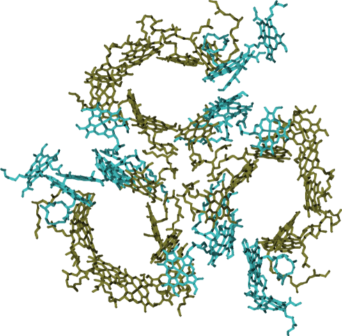
Figure 1: The chains of Chls in the trimeric LHCII. Blue: CHls-b; green: CHls-a.

The LHCII crystal structure has been determined up to $2.5\,{\AA}$ in resolution LHCIIcrystal1 ; NatureSpinach : it is composed of three similar monomeric subunits (Lhcb1-3) each containing 14 Chls molecules embedded in a protein matrix (see Fig.1). Two different types of Chls are present: $8$ Chl-a type, and $6$ Chl-b type. The main difference between the two is the presence in Chl-b of a carbonyl group that allows for higher excitation energies. The Chls are disposed in two layers which are called stromal and lumenal, the first being oriented towards the outer part of the thylakoid membrane, the second towards its inner part (see fig. 2).

Within each layer, the Chls can be grouped on the basis of their relative distance and orientations which determine the strength of the electronic interaction. The main groups of Chls are depicted in fig. 3; different groups have different linear absorption spectra and two main bands can be identified: the Chl-a band centered at $14925\,cm^{-1}$, and the Chl-b band centered at $15385\,cm^{-1}$.

Figure 2: LHCII monomer in the membrane, and its top and bottom view. Blue: CHls-b; green: CHls-a

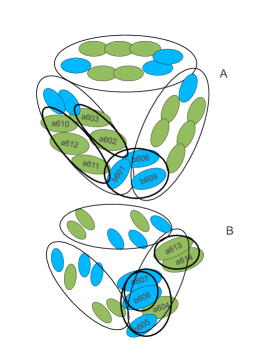
Figure 3: Stromal (A) and lumenal (B) layers of the LHCII. The groups of strongly coupled Chls are enclosed in thick circles.

The exciton energies and the relative pigment participations in LHCII have been determined in Exciton09 . The energy relaxation pathways of the system were described by van Grondelle (see Grondelle06 ) and refined in Fleming09 by means of the experimental data obtained by applying 2D spectroscopic techniques to samples of LHCII at $77K$; in the same paper, the Hamiltonian for the monomeric unit we will use in the following was also derived and optimized in order to account for the experimental results. The Hamiltonian is written in the site basis: the diagonal terms are the site energies, determined by fitting the linear absorptions spectrum and the off-diagonal terms account for the Coulomb interactions between pairs of Chls (see Fleming09 and references therein). The experimental evidences allows to identify two main downhill relaxation pathways Grondelle06 ; Fleming09 . One takes entirely place at the stromal level (stromal-stromal) while the second starts in the lumenal level (lumenal-stromal) (see fig. 4).

One of the fundamental mechanisms that is at the basis of the energy transfer through the LHCII is given by the interplay between strong electronic couplings between nearby Chls. The coupling allows both for the energy splitting between excitonic levels and for the exciton delocalization. If we focus for example on the group of Chls $a610,a611,a612$ (fig. 3) we see that the contiguity and the relative orientation of these molecules result in a strong interaction which in turn it allows for the presence of three exciton levels (levels $5,2,1$ in fig. 4) which are separated in energy and at the same time are spatially overlapping. In presence of exciton-exciton coupling, for example mediated by the environment, the spatial overlap allows for fast ($<100fs$) relaxation processes within the group-excitonic band (levels $5,2,1$ in fig. 4).

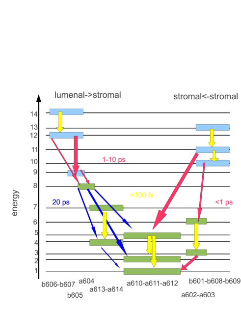
Figure 4: Energy relaxation pathways as experimentally determined in Fleming09 .

The same mechanism can be seen in another group of Chls $b601,b608,b609$ which allows for a fast ($<100fs$) relaxation process within the stromal b-band (levels $13,11,10$ in fig. 4).

In analogy with what happens for the previous groups of Chls, the intra-group energy pathways can be described by the same mechanism. In particular, in the lumenal-stromal pathways, one can identify a bottleneck of the pathway that is given by the Chls $b605$ and $a604$; here the interaction between the two molecules gives rise to a pair of well localized excitonic states (levels $8$ and $9$ in fig. 4) which have poor spatial overlap with the lower energy states concentrated on the Chl-a groups in the lumenal and the stromal side. The localization of the wave function gives rise to the experimentally determined slowdown in the relaxation process relative to the lumenal-stromal pathway. The dynamics of the bottleneck will be seen in action in the simulations of exciton transport through the monomer in the next section.

The lowest energy states of the monomer are two of the excitonic states localized in the $a610,a611,a612$ group of Chls. These sites are therefore indicated as the output sites of the monomer unit (donors), which can be coupled to other LHCII monomeric units, or other complexes in the PSII. The coupling can be between exitonic states corresponding to similar energies but located on different neighbouring complexes. In Fleming09 these two output states have been studied in terms of their directionality, which is determined by the interplay between the site basis contribution to the specific excitonic state (delocalization over the group of Chls $a610,a611,a612$) and the relative orientation of the donor transition dipoles. The result of the calculations showed that the two excitons can act as donor states in two different directions, and this mechanism has been suggested as a way that LHCII complexes have to optimize the exciton transfer to other complexes even in presence of their misalignment. In our analysis we want to compare two different ways in which the monomer can be coupled with the outer complexes: $i)$ a sites based coupling, where each output site (Chls $a10,a611,a612$) is independently coupled with an external complex that we model as a sink; $ii)$ an exciton based coupling, where the two lowest excitonic states are independently coupled with an outer sink.

For the inter-monomeric couplings, the experimental evidences in NatureSpinach (Fleming09 ), show that the main coupling should be localized in the stromal side between Chls of b type ($b601,b608,b609$); the strength of the coupling should be of the order of $42cm^{-1}$, ($35cm^{-1}$). In Fleming09 this inter-monomeric coupling has been neglected in the determination of the single monomer Hamiltonian. While this has the effect of shifting the excitonic b-band, it should not significantly affect the other transitions which are localized within each monomer. In order to have a description of the whole trimeric LHCII, we reintroduce the coupling between Chl-b pertaining to different adjacent monomers; in particular we choose two different configurations: $b601\leftrightarrow b609$ and $b601\leftrightarrow b609,b608$.
We finally note that another Hamiltonian for the LHCII complex has been derived in RengerLHCIIsinks10 . However the results that can be obtained in the following analysis by using the data reported in RengerLHCIIsinks10 instead of the ones reported in Fleming09 do not change in a significant way.

IV Model and tools

In the following we will focus on transport properties of the monomeric, dimeric, trimeric and tetrameric LHCII systems. We study the dynamics of the open quantum system in the presence of dephasing processes (Haken- Strobl formalism) in the presence of recombination and trapping mechanisms. In this model we resort to the description used in SethFMO1 ; SethFMO2 , where recombination and trapping processes are modeled by adding non-Hermitian terms to the Hamiltonian. The effects of static disorder will be taken into account below. The equation of motion for the density matrix of the monomer subunit can be written as

$$\frac{d\rho}{dt} = \frac{-i}{\hbar}\left[H_{monomer},\rho(t)\right]+L_{deph}\rho(t)-\left\{H_{recomb}+H_{trapping},\rho\right\}\equiv$$ (1)

$$\equiv L[\rho(t)],$$

The free Hamiltonian of the monomer is a tight binding Hamiltonian and it is expressed in terms of the site energies and couplings given in Fleming09

$$H_{monomer}=\sum_{m}\epsilon_{m}|m\rangle\langle m|+\sum_{m<n}V_{mn}(|m\rangle\langle n|+h.c)$$ (2)

The term

$$L_{deph}\rho(t)=\gamma_{\phi}\sum_{m}A_{m}\rho(t)A_{m}^{\dagger}-\frac{1}{2}\left\{A_{m}A_{m}^{\dagger},\rho(t)\right\},$$ (3)

accounts for the presence of pure dephasing, $A_{m}=|m\rangle\langle m|$. The term

$$H_{recomb}\equiv-i\Gamma\sum_{m}|m\rangle\langle m|,$$

accounts for the recombination processes. For the trapping, we suppose that once the exciton has reached the output sites $a610,a611,a612$, it leaves the LHCII complex with a rate $k_{trap}$. The trapping process can be expressed either with respect to the site basis i.e., the sites $a610,a611,a612$ are supposed to be singularly linked with other surrounding complexes

$$H_{trapping}\equiv-ik_{trap}\sum_{m=610,611,612}|m\rangle\langle m|,$$ (4)

or with respect to the two lowest exciton eigenstates that are localized in the $a610,a611,a612$ sites:

$$H_{trapping}\equiv-ik_{trap}(|E_{1}\rangle\!\langle E_{1}|+|E_{2}\rangle\!\langle E_{2}|).$$ (5)

The main difference between the two pictures should be that with the site-based trapping mechanism the sink acts on the output sites, including the case where only the highest exciton localized on the output states (number $5$ in figure 4) is populated. By contrast, with the excitonic-based mechanism only the two lowest energy excitonic states are involved in the trapping dynamics.

The functionals we use to evaluate the efficiency of the transport are the efficiency $\eta$, defined as

$$\eta=2k_{trap}\sum_{m}\int_{0}^{\infty}dt\langle m|\rho(t)|m\rangle$$ (6)

and the average transfer time $\tau$, defined as

$$\tau=\frac{2}{\eta}k_{trap}\sum_{m}\int_{0}^{\infty}dt\,t\,\left\langle m|\rho(t)|m\right\rangle$$ (7)

The system dynamics and the efficiency $\eta$ can be evaluated numerically by vectorizing the density matrix and constructing the proper linear super operator associated to $L$

$$\rho(t)\rightarrow|\rho(t)\rangle\rangle$$

$$L\rightarrow\mathcal{L}$$

$$|\frac{d\rho(t)}{dt}\rangle\rangle=\mathcal{L}|\rho(t)\rangle\rangle\implies|\rho(t)\rangle\rangle=e^{\mathcal{L}t}|\rho(0)\rangle\rangle.$$

$\mathcal{L}$ has been constructed using the identity $|ABC\rangle\rangle=A\otimes C^{t}|B\rangle\rangle,$ where A,B and C are matrices of size n and $|\cdot\rangle\rangle$ is a vector of size $n^{2}.$ We can now compute $\eta$ in terms of $\mathcal{L}$ as

$$\eta=-2k\sum_{m}\langle\langle m|\mathcal{L}^{-1}|\rho(0)\rangle\rangle.$$

Before passing to analyze the results of our simulations a comment on the monomer Hamiltonian is in order. The Hamiltonian given in Fleming09 has been obtained after many optimization processes with the goal of faithfully reproducing the 2-D spectroscopy experimental results. This implies that the actual eigenstates that can be derived by diagonalizing the Hamiltonian are delocalized over groups of Chls which are sometimes different by the ones showed in fig. 4, where the relative pigment participations are derived via other optimization processes. The differences manly involve the highest energy eigenstates of the b lumenal and stromal band. In our analysis, we stick to the experimentally optimized Hamiltonian and use its actual eigenstates; the spectrum of the monomer and the trimer is given in figure 5.

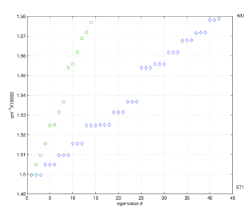
Figure 5: Energy levels for the Hamiltonian of the monomer and the trimer.

The maximal, minimal and average difference in energy for the monomer are $\Delta_{min}\approx 4cm^{-1},\Delta_{max}\approx 172cm^{-1},\Delta_{Av}=59cm^{-1}$ ($k_{B}T\approx 200cm^{-1}$ at room temperature). The differences in energies for the dimer and the trimer are very similar.

In order to study the dynamics of the monomer we make use of well established quantum information measures of correlations. In particular, we measure the total amount of correlations between two subsystems of chromophores $A$ and $B$ with the quantum mutual information NielsenChuang

$$\mathcal{I}_{AB}=\mathcal{(}S)_{A}+\mathcal{(}S)_{B}-\mathcal{(}S)_{AB}$$ (8)

where $\mathcal{(}S)_{X}=\sum_{i}\lambda_{i}\log_{2}{\lambda_{i}}$ is the von Neumann entropy of the reduced density matrix $\rho_{X}$ of subsystem $X$ evaluated in terms of its eigenvalues $\{\lambda_{i}\}$. As for the quantum correlations between subsystems composed by arbitrary number of chromophores we use the negativity $\mathcal{N}_{AB}$ vidalvernerneg that in the single exciton manifold can be written as Caruso10

$$\mathcal{N}_{AB}=\sqrt{a_{00}^{2}+4\sum_{n=1}^{k}\sum_{m=k+1}^{N}|\left\langle n|\rho_{AB}|m\right\rangle|^{2}}-a_{00}$$ (9)

where $a_{00}$ is the element corresponding to the zero exciton subspace and $A=1,\cdots,k$, $B=k+1,\cdots,N$ are two generic subsystems of chromophores. The quantum correlations between pairs of sites $m,n$ are also measured by means of the concurrence WoottersConcurrence which in the single site exciton has the simplified form Sarovar10

$$\mathcal{C}_{m,n}=2|\rho_{m,m}|.$$ (10)

In order to study the relationship between the dynamics of the above described correlations measures and the delocalization of the exciton over the monomeric structure we define a measure of delocalization $\mathcal{D}(t)$ that involves the single site populations. In keeping with this paper’s methods of using information-based measures to characterize the excitonic transport, we use Shannon entropy as a measure of delocalization. If $\left\langle n_{i}\right\rangle$ is the population of site $i$ at time t, then by using the normalized populations $\lambda_{i}=\left\langle n_{i}\right\rangle/\sum_{i}\left\langle n_{i}\right\rangle$ we can define

$$\mathcal{D}(t)=-\sum_{i}\lambda_{i}\log{\lambda_{i}}$$ (11)

as the Shannon entropy of the normalized populations. The higher $\mathcal{D}(t)$, the flatter the probability distribution $\{\lambda_{i}\}$, the higher the delocalization of the exciton over the complex.

V Monomer dynamics

In the following we describe the dynamics of the monomer. The values of the recombination and trapping coefficients used for the simulations are the ones used for the FMO complex in SethFMO1 ; IshiFleming10 . The recombination coefficient $\Gamma=10^{-3}ps^{-1}$ takes into account the estimated lifetime of the exciton, $1ns$. The trapping coefficient is $k_{trap}=1ps^{-1}$ and is assumed to be equal for each output exciton state. Our results do not depend sensitively on the exact value of the exciton lifetime and the trapping rate: what is important for the analysis is that the exciton has a relatively long lifetime compared with coupling rates, and that the trapping rate is comparable to those rates.

We first focus on the time simulation of the evolution of the monomer in order to identify the possible energy transfer pathways. We therefore fix the value of the dephasing rate $\gamma_{\phi}\approx 3ps^{-1}$ that corresponds to $77K$ (temperature at which the experiments were done in Fleming09 ). The dephasing rate can be written in terms of the bath correlation function as SethFMO2 :

$$\gamma_{\phi}(T)=2\pi\frac{k_{B}T}{\hbar}\partial_{\omega}J(\omega)|_{\omega=0}=2\pi\frac{k_{B}T}{\hbar}\frac{E_{r}}{\hbar\omega_{c}}$$ (12)

where we have supposed to have an Ohmic correlation function $J(\omega)=\pi\frac{k_{B}TE_{r}}{\hbar}\frac{\omega}{\omega_{c}}\exp{\omega/\omega_{c}}$ (super- and sub-Ohmic correlation functions give a similar dependence on $T$, $E_{r}$, and $\omega_{c}$). The recombination energy $E_{r}=35cm^{-1}$ and the cut-off frequency $\omega_{c}=150cm^{-1}$ are chosen to be the ones used for the FMO simulations. Again, the qualitative behavior of the excitonic transport does not depend sensitively on the precise values of $E_{r}$ and $\omega_{c}$.

V.1 Energy and correlation pathways

We want to describe the time evolution of the state of the monomer coupled with the environment. We first try to identify and characterize the existence of two possible pathways, stromal-stromal and lumenal-stromal, by which the exciton, starting from a high energy state belonging to the b band, can reach the output sites. We therefore focus our attention on the behaviour of the system without any trapping and for a value of the dephasing rate that corresponds to the temperature of $77K$ used in Fleming09 . As noted above, since the Haken-Strobl model is purely dephasing and does not include an explicit relaxation term, we expect our analysis to underestimate the rate of transfer from high energy states to low energy states. Nonetheless, as will now be seen, pure decoherence gives efficient excitonic transport down the energy ladder.

The distinct pathways can be studied by plotting the following populations: $i)$ the populations of the excitonic states which are mostly localized on Chl-b molecules that belong to the stromal (lumenal) side $P_{bStrom}(P_{bLum})$ $ii)$ the populations of the excitons states which are mostly localized on Chl-a molecules that belong to the stromal (lumenal) side $P_{aStrom}(P_{aLum})$.

The different excitonic behaviors along the two distinct pathways can also be highlighted by using measures of quantum correlations. In particular, we study the quantum mutual information between the relevant subsystems that are naturally suggested by the energy landscape in fig. 4; in this way we can identify the correlation pathways and their dynamics. On the lumenal side we select the subsystems $bL=\{606,607\},abL=\{605,604\},aL=\{613,614\}$, while on the stromal side we select the subsystems $bS=\{601,608,609\},aintS=\{602,603\},aoutS=\{610,611,612\}$ and $aS=aintS\cup aoutS$; the bipartitions are schematically depicted in fig. 6. The growth of quantum correlations between subsystems is a signature of the spreading of the initially localized exciton between subsystems. The form that these correlations take over time reveals the mechanism of this spreading – an almost purely coherent initial propagation followed by semi-coherent diffusion.

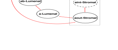
Figure 6: Schematic picture of the bipartitions used for the analysis of correlations dynamics

For the stromal-stromal pathway we choose as initial state of our simulations the highest energy eigenstate $|E_{14}\rangle$ of the Hamiltonian, which is mostly localized on the $b601$ Chl. In Fig.7 we see how the exciton mostly flows from the stromal b-band to the stromal a-band on a very short time scale ($\approx 5ps$). On a slower time scale the population partially delocalizes over the lumenal band. The flow of population between the two b-bands was highlighted in the energy pathway given in Grondelle06 (but not highlighted in Fleming09 ), where the possibility of a flow from the b-lumenal to the b-stromal band is estimated to be of the order of $2ps$. Here we observe the inverse passage b-stromal to b- lumenal and this is due also to the partial delocalization of the $|E_{14}\rangle$ on the b-lumenal sites. The global population decreases because of excitonic decay with a time scale of the order of $1ns$.

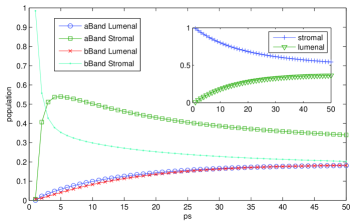
Figure 7: Stromal-Stromal pathway: populations for initial state $|E_{14}\rangle$

The dynamics can be further analyzed by considering the correlation pathways. Figure 8 refers to the stromal-stromal pathway starting with $|E_{14}\rangle$. The plots shows that the dynamics mostly takes place on the stromal side. In particular (left plot) the $bS$ subsystem initially gets correlated with a-band stromal sites as a whole ($MIaSbS$); in the first few picoseconds most of the correlations are established between the subsystems $bS$-$aintS$, and the subsystems $aintS$-$aoutS$. From the first picosecond on the $bS$ sites get directly correlated with the output sites $aoutS$. The right plot in fig. 8 shows that while there are correlations between the stromal and the lumenal b-bands ($MIbLbS$), the correlations among the subsystems on the lumenal side and the lumenal-stromal correlations at the level of the a-bands are negligible ($\approx$ one order of magnitude smaller). This picture is consistent with a dynamics mostly localized on the stromal side of the monomer.

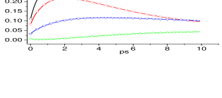
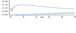
Figure 8: Stromal-Stromal pathway: mutual information for initial state $|E_{14}\rangle$; left: stromal side; right: lumenal side

We now pass to analyze the behaviour of the system when the exciton starts on a a high energy eigenstate $|E_{13}\rangle$ which is mostly localized on the lumenal side (in particular on the site $b606$). The behaviour of the populations shown in fig. 9 accounts for the presence of a bottleneck in the energy pathways Fleming09 ; Grondelle06 . The latter is due on one hand to the high spatial localization of the exciton involving the site $a604$ (which is far from the other a-lumenal sites), and on the other hand to the large energy separation with respect to the excitons localized on the neighbouring lumenal sites $b605,b606,b607$ ($\Delta E\approx 172cm^{-1}$ eigenvalue $8$ with respect to eigenvalue $9$ in fig. 5). Indeed, while in the first few picoseconds, the population of the b-lumenal sites decreases in favor of the population of a-lumenal band, part of the b-lumenal population start to flow toward the b-stromal band. The overall effect is that the a-stromal sites, and therefore the output sites, become populated with a smaller rate than in the stromal-stromal case.

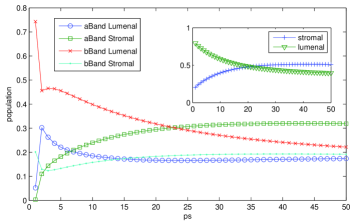
Figure 9: Lumenal-Stromal pathway: populations for initial state $|E_{13}\rangle$

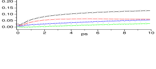
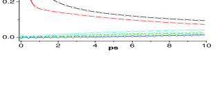
Figure 10: Lumenal-Stromal pathway: mutual information for initial state $|E_{13}\rangle$; left: stromal side; right: lumenal side

The trapping effect on the lumenal side can also interpreted in terms of correlation pathways. As it is shown in the right plot of fig. 10 the b-lumenal band is initially highly correlated with the b-stromal band (black line, right plot).

On one hand this is due to the fact that the eigenstate $|E_{13}\rangle$ is partially delocalized on the sites $b608,b609$. On the other hand, as already mentioned, the b-lumenal to b-stromal flow, was already pointed out in terms of energy pathways in Grondelle06 , where the transfer time between b-lumenal sites and b-stromal sites were estimated of the order of $2-4ps$, and, despite the small level of interaction ($\leq 11cm^{-1}$, see Ham) it is consistent with the contiguity of the b-lumenal and b-stromal sites in the monomer.

While the correlations between b-lumenal and b-stromal bands rapidly decay in the first few picoseconds, there is not a corresponding growth of correlations on the lumenal side: the b-lumenal and a-lumenal sites remain very poorly correlated among each other and with the rest of the a-stromal sites. At the same time there is a clear enhancement of the correlations on the stromal side, which become rapidly greater than those on the lumenal side, suggesting the activation of the stromal-stromal pathway.

The above analysis is robust with respect to the choice of the initial state; for example in fig. 11 the same simulations have been carried out for an initial state $|b607\rangle$ fully localized on the b-lumenal site $b607$. Here the activation of the stromal-stromal pathway is evident; in the first $1ps$ the b-lumenal subsystem gets correlated both with the sites $b605,a604$ ($MIabLbL$)and with the b-stromal band ($MIbLbS$ right plot); then the correlations are mostly built on the stromal side (left plot) while on the same time scales the correlations with the output sites on the lumenal side are build with a slower rate.

The net effect of the presence of the above mentioned bottleneck on the lumenal side is a substantial slowdown of the lumenal-stromal dynamics. There are a number of possible functional advantages for this slowdown. One possibility is to assist in photoprotection, the elimination of triplet exciton states that can create harmful singlet oxygen. This elimination takes place primarily by the transfer of triplet excitons to triplet carotenoid states, and has a relatively slow timescale (a fraction of a microsecond) compared with singlet exciton transfer Photoprotect1 . Triplet transfer is a Dexter process, mediated by wave function overlap, and requires the carotenoids to be physically close to the chromophore carrying the triplet. X-ray crystallography studies of LHCII suggest that the $a604$ chromophore in the lumenal bottleneck is close enough to a lutein carotenoid to allow triplet transfer, a process confirmed by spectroscopy NatureSpinach ; Photoprotect1 .

A second possible function for the lumenal bottleneck is that the bottleneck $b605$ chromophore could mediate excitonic transport from one trimer to another NatureSpinach . This chromophore ‘sticks out’ from the others in the LHCII crystallographic structure, giving both weaker couplings to the other chromophores within the LHCII monomer, and potentially stronger couplings to chromophores in neighboring triples. Crystallographic investigations of LHCII suggest that the $b605$ is positioned to transfer excitons to the $b606$ and $a614$ chromophores of neighboring trimers in LHCII aggregates NatureSpinach . This transfer pathway could also participate in photoprotection via non-photochemical fluorescence quenching.

A third possible reason for the slower lumenal pathway is that it might allow two excitons to propagate through the LHCII complex simultaneously without quenching. The weak coupling between the bottleneck chromophores of the lumenal pathways and the chromophores of the stromal pathway, together with their relative spatial separation, could allow an exciton localized in the lumenal pathway to wait for a stromal exciton in the same complex to pass through the stromal trapping states, before passing through itself.

To summarize, the dynamics of the slow lumenal side and the fast stromal side have many have a rich set of potential biological functions. These dynamics are in turn based on a rich quantum structure, which the next section elucidates.

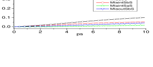
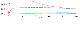
Figure 11: Lumenal-Stromal pathway: mutual information for initial state $|b607\rangle$; left: stromal side; right: lumenal side

V.1.1 Delocalization and quantum correlations

In the following we examine the monomer dynamics from the point of view of the time scales that characterize the delocalization of the excitons over the whole monomeric structure and the quantum correlations between the various subsystems. In order to estimate the delocalization time we plot the populations of the various bands in fig. 12 (left plot), and the previously defined measure of delocalization $\mathcal{D}(t)$ (11). Since we want to study the dynamics of the spreading of the correlations we first focus on the initial state $|b601\rangle$ localized on the Chl $b601$ only. We choose this state because it is very close to the highest energy eigenstate $|E_{14}\rangle$, which is mostly localized on the same site but has non-negligible quantum correlations with the rest of the system. We want to start with a state localized on a single chromophore, in order to study how the correlations spread through the structure. In fig. 12 we plot the delocalization function $\mathcal{D}(t)$ for $\gamma_{\phi}=3ps$ ($\approx 77K$), $\Gamma=0.001$ and no trapping. The delocalization has a very fast growth and it can be well represented by a function $\mathcal{D}(t)=y0+A1\exp{-t/t_{1}}+A2\exp{-t/t_{2}}$ where two time scales $t_{1}\approx 250fs$ and $t_{2}\approx 2.68ps$ appear. The relevance of these time scales can be understood by studying the quantum correlations between the relevant subsystems.

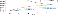
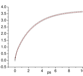
Figure 12: Initial state $|b601\rangle$ ($\approx|E_{14}\rangle$), state localized on the Chl $b601$ on the stromal side. Populations (left) and delocalization (right) $\mathcal{D}(t)$ with fitting curve.

,

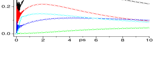
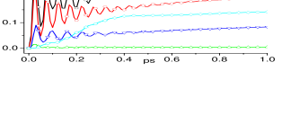
Figure 13: Initial state $|b601\rangle$ ($\approx|E_{14}\rangle$), state localized on the Chl $b601$ on the stromal side. Mutual information between subsystems on the stromal side and between b-lumenal and b-stromal band ($MIbLbS$); the right plot displays the dynamics during the first $1ps$.

In the left panel of fig. 13 we plot the mutual information for the relevant subsystems over a time of $10ps$. As it can be easily seen, the second time scale $t_{2}\approx 2.68ps$ can be correlated with the growth of the mutual information between the various subsystems which reach its maximum at a time $t$ very close to $t_{2}$. In particular the correlations between the b-band and the a-band on the stromal side has a maximum at $t\approx 2.63ps$. In the right panel of fig. 13 we show the dynamics of correlations within the first picosecond. Here the dynamics displays an initial fast growth of all correlations ($\approx 0.50ps$) which are characterized by an oscillating behaviour; the time scale of these oscillations is of the order of $0.1ps$. These oscillations are signatures of the high degree of quantum coherence in the initial spreading. The growth becomes regular within the first $400fs\approx 1.5t_{1}$; within the same period of time the correlations spread toward the lumenal side ($MIbLbS$)

The overall effect can therefore be described in terms of the two relevant timescales: the delocalization takes place over the structure with an initial fast rate, and subsequently it grows toward its asymptotic behaviour with a slower rate. The time scale of the initial rapid and oscillating growth is consistent with the dynamics of the quantum correlations present in the system. In fig. 14 (left plot) we show the behaviour of the negativities among the relevant subsystems over the first $10ps$ (NegbLbS is the negativity between the lumenal and the stromal b-bands). In the first picosecond (right plot), after a first rapid growth ($\approx 50fs$ ) they show the same oscillatory behaviour of the mutual information and they then decay in a smooth way after the first $\approx 400ps$ (left plot). This behaviour is also shown by the concurrences between sites: in fig. 15 we show the relevant (non-negligible) concurrences between the site $b601$ and other sites. Non-zero negativity and concurrence demonstrate the presence of entanglement during the initial coherent spreading, similar to the presence of entanglement in FMO Sarovar10 ; Caruso10 . The quantum correlations are therefore established in the first few hundreds of femtoseconds and they give their contribution for the first rapid growth of the delocalization of the exciton over the whole structure (stromal and lumenal side).

,

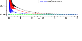
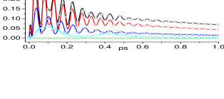
Figure 14: Initial state $|b601\rangle$ ($\approx|E_{14}\rangle$), state localized on the Chl $b601$ on the stromal side. (Un-normalized) Negativities between subsystems on the stromal side and between b-lumenal and b-stromal band ($NegbLbS$); the right plot displays the dynamics during the first $1ps$.

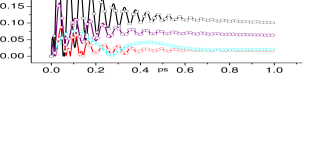
Figure 15: Initial state $|b601\rangle$ ($\approx|E_{14}\rangle$), state localized on the Chl $b601$ on the stromal side. Relevant, i.e. non-negligible, concurrences between site $b601$ and other sites on the stromal ($b603$,$b11$) and lumenal ($b606$) sides; the plot displays the dynamics during the first $1ps$.

V.2 Effect of the trapping on the monomer dynamics

In order to see how the trapping modifies the monomer dynamics we focus on the stromal-stromal dynamics. The initial exciton state is $|E_{14}\rangle$ and we choose to fix the value of the dephasing rate to $\gamma_{\phi}=12ps^{-1}$ (that approximately corresponds to the ambient temperature if one uses 12). In fig. 16, the left plot displays the populations of the various subsystems. The comparison of the populations dynamics with the site based trapping mechanism and the exciton based mechanism shows that the first one is obviously more efficient in reducing the total population and the population of the various band (in particular the a-lumenal one). As noted above, this difference arises in our model because site-based trapping operates on three sites, while the exciton based mechanism acts only when the two lowest eigenstates get populated.

In the right plot of fig. 16 we show the delocalization functional for no trapping and for site/exciton based trapping. The presence of the trapping mechanism starts to be relevant already after the first picosecond, i.e. before the full delocalization of the exciton has occurred. Indeed for $\gamma_{\phi}=12ps^{-1}$ the typical time scales of the delocalization without trapping are $t_{1}\approx 400fs$ and $t_{2}\approx 1.5ps$. This means that, in presence of trapping, the delocalization due to the initial dynamics of the quantum correlations has a fundamental role in the energy transfer process.

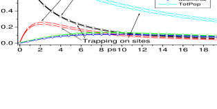
Figure 16: Initial state $|E_{14}\rangle$. Dephasing $\gamma_{\phi}=12ps^{-1}$; trapping $k_{trap}=1ps^{-1}$; recombination $\Gamma=0.001ps^{-1}$. Left: populations of the different bands with exciton/site base trapping; right: delocalization functional $\mathcal{D}(t)$ with exciton/site base trapping and no trapping

V.3 The monomer as wire

An interesting problem is to determine the typical time scales that govern the delocalization of an exciton initially localized on the output sites $a610,a611,a612$ of the monomer. These quantities become relevant when one describes the behaviour of the dimer and the trimer when they act as quantum wires. Indeed, the LHCII complex can in principle be activated by other neighbouring LHCII complexes and this should happen when the output sites of a pair of LHCII are sufficiently close. In this process, the $a610$, $a611$, and $a612$ sites on an LHCII monomer accept an exciton from the same sites on a neighboring trimer. The exciton then spreads first through the monomer, and then throughout the three LHCII units of the trimer. When it reaches another set of output sites, the exciton can be transferred to another trimer, and the process repeats.

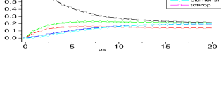
Figure 17: Initial state $|E_{1}\rangle$, ground state of the monomer localized over the output sites. Populations of the different subsystems and delocalization functional $\mathcal{D}(t)$

Accordingly, we now analyze the interaction between donors $a610,a611,a612$ on one monomer within the trimer, and “acceptor” $a610,a611,a612$ sites on a second monomer within the trimer. The acceptor LHCII sites behave as a sink with a trapping rate that depends on how fast the exciton localized on those “acceptor” sites diffuses to a neighboring LHCII trimer or to some other part of the overall photocomplex. In order to study this diffusion process, we first focus on a single monomer, initialized in the monomer Hamiltonian ground state $|E_{1}\rangle$ (localized on $a610,a611,a612$). In order to estimate the delocalization time we plot the populations of the various bands in fig. 17 (left plot). We use the previously introduced delocalization measure $\mathcal{D}(t)$ which is plotted in the right part of fig. 17. The simulations employ a fixed value of the dephasing rate $\gamma_{\phi}=12ps^{-1}$ that approximately corresponds to ambient temperature. The population of the acceptor sites decreases and becomes of the same order of the other populations in about $10ps$. If we take $\mathcal{D}(t)=y0+A1\exp{t/t_{1}}+A2\exp{t/t_{2}}$ to estimate the delocalization process over the whole monomer ($\mathcal{D}(t)$ is a site based measure of delocalization) we see that the relevant time scale $t_{2}\approx 2ps$ (while for the initial fast growth we have $t_{1}\approx 350fs$).

The value of $t_{2}$ is of the same order of the inverse of the trapping rate which is characteristic of the FMO $k_{trap}^{-1}=1ps$ that we used for the monomer in the previous section, and that we will use for the dimer, the trimer and the tetramer in the following section.

VI Efficiency: a comparison between clusters of monomers

In this section we examine the efficiency and typical transfer time of the single monomer and of groups of 2, 3, and 4 monomers. The clusters are build by connecting monomeric subunits via a site-site interaction: as pointed out in Fleming09 there is evidence of a relatively strong coupling in the cluster $\{b601,b608,b609\}$, where $b601$ belongs to one monomer and $\{b608,b609\}$ to another one. In NatureSpinach , where the LHCII of the spinach is analyzed, the link between the $b601$ and the $b609$ sites is estimated to be $42\;cm^{-1}$. We therefore write the overall Hamiltonian of the complex, say the trimer, as:

$$H_{trimer}=\sum_{i=1,2,3}H^{i}_{monomer}+H_{12}^{int}+H_{23}^{int}+H_{31}^{int},$$ (13)

where the terms $H_{ij}^{int}=V_{b601_{i},b609_{j}}(|b601_{i}\rangle\!\langle b609_{j}|+|b609_{j}\rangle\!\langle b601_{i}|$ account for the Coulomb interaction between the Chl $b601$ on the $i-th$ monomer and the Chl $b609$ on the $j-th$ monomer. $V_{b601_{i},b609_{j}}$ is chosen to be equal to $42cm^{-1}$ Fleming09 . We will also consider the case when the coupling $b601-b608$ is present and equal to $42cm^{-1}$.

The recombination parameter is fixed at $\Gamma=0.001ps^{-1}$, which again is the value used for the FMO in SethFMO2 . Trapping is supposed to be similar to the monomeric case; the output sites are now the group of sites $a610,a611,612$ on each monomer, and the trapping Hamiltonian is $\sum_{i}k_{trap}(|a610_{i}\rangle\!\langle a610_{i}|+|a611_{i}\rangle\!\langle a611_{i}|+|a612_{i}\rangle\!\langle a612_{i}|)$, where $i$ labels the monomers, with $k_{trap}=1ps^{-1}$.

The main result of these simulations is that there is a clear evidence for a dephasing-assisted mechanism that enhances the transport efficiency of the systems. This mechanism is an example of environmentally assisted quantum transport (ENAQT) SethFMO1 ; SethFMO2 ; Plenio08 . The result is independent of the structure analyzed. Efficiencies and the average transfer times have their optimal values in correspondence of a dephasing rate $\gamma_{\phi}\geq 10ps^{-1}$, i.e. the rate corresponding to ambient temperature.

VI.1 The antenna configuration

We first describe the efficiency of the various complexes when they act as antennae. We start by focusing on the relevant figures of merit for the single monomeric unit. In fig. 18 we show the efficiency (left) and the average transfer time (right) for two different initial states: $|E_{14}\rangle$, mostly localized on the stromal side and $|E_{13}\rangle$, mostly localized on the lumenal side. The plots show that the differences highlighted by our analysis of the dynamics in the previous section have relevant effects also in terms of the transport efficiency of the monomer. The stromal-stromal pathway that starts with $|E_{14}\rangle$ results in general in a better efficiency and a smaller $\tau$ over the whole range of dephasing rates. In particular, at $\gamma_{\phi}\geq 10$ $\tau$ is $\approx 1.5$ times smaller than the corresponding lumenal-stromal value. The mismatch in the characteristic time of the two pathways arises from the bottleneck present in the lumenal pathway.

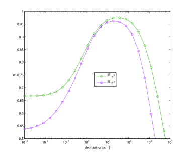
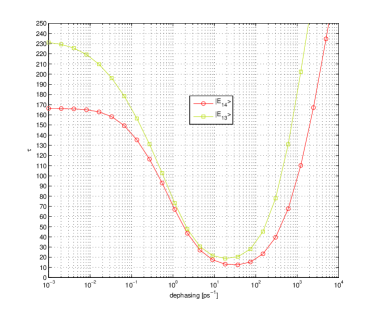
Figure 18: Efficiency $\eta(\gamma_{\phi})$ (left) and Average transfer time $\tau(\gamma_{\phi})$ (right) for the monomer with different initial states: $|E_{13}\rangle$ (mostly localized on the lumenal side) and $|E_{14}\rangle$ (mostly localized on the stromal side).

We now describe in detail the results of our simulations for more complex structures. We first examine the case in which there is an active sink attached to each of the monomers of a given structure. The initial state used for the various simulations is the highest excited state of the Hamiltonian, which is basically a copy over different monomers of the eigenstate $|E_{14}\rangle$ of one single monomer: it is thus mainly localized on the b-stromal Chls of each structure. In Fig. 19 (left) we compare the efficiency of the energy transport for different geometries in presence of only one inter-monomeric coupling. While the dephasing assisted mechanism is always present, we see that for physically relevant values of the dephasing parameter the change of geometry does not provide significant modifications in the efficiency. Fig. 19 (right) shows the result of the simulations for $\tau$, the characteristic transfer time. The value corresponding to the highest efficiency in the transport is around 10-15 ps. This transport time is consistent with that observed for the FMO complex, taking into account the fact that each monomer subunit of the LHCII has twice the number of chromophores of FMO.

The results we obtain in this paper are robust with respect to the introduction of static disorder. In Fig.20 we add the effects of static disorder (on site-energy values) and compare the efficiency for different numbers of monomers. The strength of disorder is taken to be that reported in disorder . The qualitative behavior of the efficiency with disorder is the same as that without. The monomer is more affected by disorder than the dimer and trimer, indicating greater robustness for the more complicated geometries. This is consistent with the fact that fluctuations due to disorder are stronger for systems of smaller size.

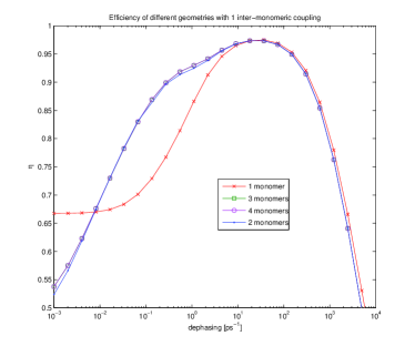
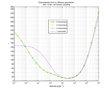
Figure 19: Efficiency $\eta$ (left) and average transfer time $\tau$ ($ps$) (right)for the different topologies (monomer, dimer, trimer and complex with 4 monomers) with single intra-monomeric coupling for various values of the dephasing rate $\gamma_{\phi}$. Initial state: highest energy eigenstate of the given structure.

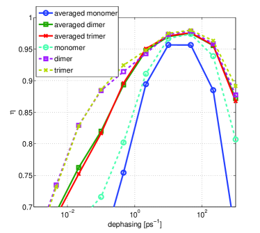
Figure 20: Efficiency $\eta$ for different topologies (monomer, dimer, trimer) in the presence of static disorder, varying the dephasing rate $\gamma_{\phi}$. Solid lines represent the averaged value, while dashed lines represent the result for the non-disordered Hamiltonian that we use in this work.

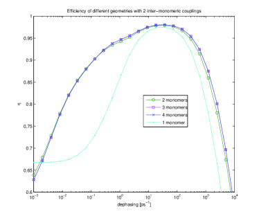
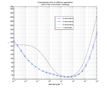
Figure 21: Efficiency $\eta$ (left) and average transfer time $\tau$ ($ps$) (right)for the different topologies (monomer, dimer, trimer and complex with 4 monomers) with two intra-monomeric coupling for various values of the dephasing rate $\gamma_{\phi}$. Initial state: highest energy eigenstate of the given structure.

Differences between the various geometries can be observed when the inter-monomeric coupling is supposed to be present between the b601 Chl in one monomer and both b608 and b609 in the neighbouring monomer, see fig. 21. The efficiency of the clusters of monomers benefits from this kind of coupling: $\eta$ is enhanced with respect the single monomer case over a wide range of dephasing values. Moreover, while the dimer is slightly less efficient than the trimer and the tetramer structures that have a higher number of traps, our simulations suggest that there is no advantage in adding more than three subunits: the trimer behaves just as well as the tetramer. This results could be an indication for a functional selection of the trimeric configuration with respect to the other ones: the trimer could be the result of an optimization with respect to the “cost” of the structure.

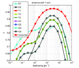
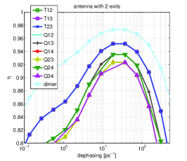
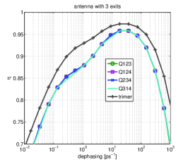
Figure 22: Efficiency of the transport for dimer, trimer and tetramer clusters, with one inter-monomeric coupling, acting as ANTENNAS In the legend Q23 means that we consider a tetrameric complex where the exciton is captured in the first monomer, and can exit only from the II and III monomers. Analoguosly for the trimer (T) and the dimer (D).

Interesting differences between the behaviour of the different structures appear when one considers a variable number of active sinks. In Fig. 22 we compare the transport in monomeric and dimeric, trimeric and tetrameric antennas with only one inter-monomeric coupling, and with different numbers of sinks attached to the available monomeric subunits. The initial state in these simulations is always the highest excited state of the structure. The main feature here is that the efficiency at physiological temperatures is always greater for the structure with a number of sinks equal to the number of monomers. For example, with a single sink attached, the monomer is more efficient than the dimer, trimer and tetramer. This behaviour is reasonable since the exciton is initially delocalized over the whole structure and in particular over those monomers that do not have any sink attached. A qualitative explanation of the relative behavior for the different configurations is based on the competition between an enhancement of the efficiency due to a greater number of sinks, and the depletion of efficiency due to a greater number of chromophores, where the exciton can delocalize and dissipate in the bath, causing a slow down in the funneling process. As already noticed, Fig. 19, the trimer saturates the enhancement of efficiency due to the number of exits: the tetrameric complex with four sinks and the trimer complex with three sinks have the same efficiency.

VI.2 The wire configuration

We now analyze the multi-monomer structures when they are used as “wires”. As noted above, the LHCII complexes can function as connecting structures between different units of the PSII complex. In the following we analyze this case by fixing as the initial state of the dynamics the ground state $|E_{1}\rangle$ of one single monomer in the cluster and by connecting a sink to each of the other monomers in the complex.

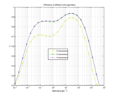
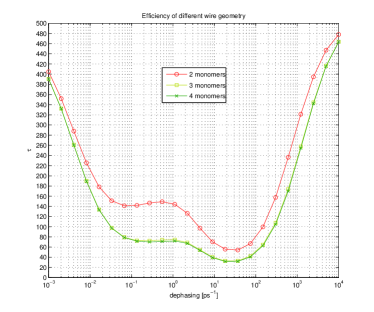
Figure 23: Efficiency $\eta$ (left) and average transfer time $\tau$ ($ps$) (right) for the different topologies (dimer, trimer and complex with 4 monomers) with single intra-monomeric coupling for various values of the dephasing rate $\gamma_{\phi}$. Initial state $|E_{1}\rangle$, i.e. ground state of a single monomer, localized on the ”acceptor” sites $a610,a611,a612$ .

Fig. 23 shows the efficiency and the characteristic time of the dimer, the trimer and of a cluster of four monomers coupled together with only one inter-monomer connection. The simulation suggests again a special role played by the trimer. It is significantly more efficient than the dimer, but almost indistinguishable from the cluster of four monomers. In the wire configuration, the exciton passing through the dimer has only one trapping site that it can reach, while in the trimer, tetramer, and higher order polymers, the exciton entering at the lowest energy site has two trapping sites that it can reach – those on the two monomers adjacent to the entrance site. Consequently, the efficiency of trapping is higher for the trimer and tetramer than for the dimer: two traps are better than one. Moreover, the dynamics for passing from the entrance site to those two adjacent traps are identical for the trimer, tetramer, and higher order polymers. Consequently, the efficiency profiles for the trimer, tetramer, and higher order polymers are identical.

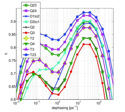
Figure 24: Efficiency of the transport for dimer, trimer and tetramer clusters, with one inter-monomeric coupling, acting as WIRES. In the legend Q23 means that we consider a tetrameric complex where the exciton is captured in the first monomer, and can exit only from the II and III monomers. Analoguosly for the trimer (T) and the dimer (D).

We finally describe how the number of attached sinks modifies the overall efficiency of the different quantum wires. In Fig. 24 the simulations refer to a situation where the initial state of the structure is the ground-state $|E_{1}\rangle$ localized in the $a610,a611,a612$ Chls of a single monomer of the structure. Here again we see a behaviour similar to the antenna confirguration case: at fixed number of sinks attached the efficiency is higher for those structures with a smaller number of chromophores . The trimer is again a limiting case, it is always more or as efficient as the tetramer, and, as already shown in fig. (23) the trimer with two sinks has the same performance of the four-monomer structure with three sinks. An analogue comparison holds true for the dimeric vs trimeric cluster. When only one sink is active, at the relevant values of dephasing – i.e. where the efficiency is maximal – the dimer can perform slightly better than the trimer. From our simulations it is also evident that, within our assumptions for the inter-monomer links, the various structures show a directionality of transport. For example the efficiency of the dimer changes significantly over a wide range of dephasing values depending on the direction of the energy flow.

VII Conclusion

We have analyzed excitonic transport in the primary component of the photosynthetic apparatus in green plants: LHCII. By means of a simple decoherence model (Haken-Strobl), the analysis shows that an exciton initially localized on a single chromophore moves through the LCHII photocomplex in a two-step process which clearly signaled by a quantum information motivated measure of delocalization. First, over the timescale of a few hundreds of picosecond, the exciton spreads coherently to neighboring chromophores. This coherent spreading exhibits rapid quantum oscillations and entanglement. Second, as the environment decoheres the exciton’s position, the exciton diffuses semi-coherently throughout the complex over a timescale of ten to twenty picoseconds. Although the Haken-Strobl model does not include relaxation, we expect this two-step, coherent–semicoherent model to hold for more detailed models of the dynamics as well, for example, in the full hierarchy approach of IshiFleming09 .

Detailed comparison of different measures of correlations also allows us to identify how the two main downhill relaxation pathways unveiled by the experiments (stromal-stromal, lumenal-stromal) can be dynamically described in terms of correlations pathways: the correlations among subsytems of pigments are mostly established on the stromal side of the monomeric complex even when the excitation is initially localized on the lumenal side. This behaviour has important consequences when the efficiency of the transport is considered: the stromal pathway is in general more efficient than the lumenal one.

In general, the analysis shows that even in the absence of relaxation, pure dephasing induces effective transport down the LHCII energy funnel. The transport is efficient and robust in the presence of static disorder, and exhibits the characteristic signature of characteristic environmentally assisted quantum transport (ENAQT) – low efficiency at low temperature due to transient localization, followed by a robust maximum efficiency at physiological temperature, with a falling off of efficiency at very high temperature. In the second part of the paper, we compared the efficiency of transport through LHCII structures with different topologies (monomers, dimers, trimers, and tetramers) and different configurations (antenna and wire). We find that the efficiency of transport increases as the number of subunits increases, saturating at the level of the trimer. These results provide evidence for the functional selection of the trimeric configuration.

References

- (1) R.E. Blankenship, Molecular Mechanisms of Photosynthesis, Blackwell Science Ltd., London, 2002.
- (2) G.S. Engel, T. R. Calhoun, E. L. Read, T. K. Ahn, T. Mancal, Y. C. Cheng, R. E. Blankenship and G. R. Fleming, Nature 446, 782 (2007).
- (3) E. Collini, C. Y.Wong, K. E.Wilk, P.M. Curmi, P. Brumer, and G. D. Scholes, Nature 463, 644 (2010).
- (4) G. Panitchayangkoon, D. Hayes, K. A. Fransted, J. R. Caram, E. Harel, J. Wen, R. E. Blankenship, G. S. Engel, Proc. Nat. Acad. Sci. 107, 12766 (2010).
- (5) M. Mohseni, P. Rebentrost, S. Lloyd, and A. Aspuru-Guzik, J. Chem. Phys. 129, 174106 (2008).
- (6) P. Rebentrost, M. Mohseni, I. Kassal, S. Lloyd, and A. Aspuru- Guzik, New J. Phys. 11, 033003 (2009).
- (7) M.B. Plenio and S.F. Huelga, New J. Phys. 10, 113019 (2008).
- (8) R. van Grondelle and V. I. Novoderezhkina, Phys. Chem. Chem. Phys. 8, 793807 (2006).
- (9) T.R. Calhoun, N.S. Ginsberg, G.S. Schlau-Cohen, Y.-C. Chen, M. Ballottari, R. Bassi, G.R. Fleming, J. Phys. Chem. B 2009, in press.
- (10) G.S. Schlau-Cohen, T.R. Calhoun, N.S. Ginsberg, E.L. Read, M. Ballottari, R. Bassi, R. van Grondelle, G.R. Fleming J. Phys. Chem. B 113, 15352 (2009).
- (11) F. Muh, M. El-Amine Madjet, and T. Renger, J. Phys. Chem. B, 2010, 114 (42)
- (12) H. Haken, G. Strobl, in The Triplet State, Proceedings or the International Symposium, Am. Univ. Beirut, Lebanon (1967), A.B. Zahlan, ed., p. 311, Cambridge University Press, Cambridge (1967).
- (13) a description of the thylakoid membrane, PSII complex and LHCII complex can be found at http://photosynthesis.peterhorton.eu/research/lightharvesting.aspx
- (14) D. Galetskiy, I. Susnea, V. Reiser, I. Adamska, and M. Przybylskia, Am. Soc. Mass. Spectrom. (2008), 19, 1004-1013; E. Romanowska, JOURNAL OF BIOLOGICAL CHEMISTRY VOL. 283, NO. 38, pp. 26037 26096, September 19, (2008); R. Danielsson et al., THE JOURNAL OF BIOLOGICAL CHEMISTRY VOL. 281, NO. 20, pp. 14241 14249, May 19, (2006) G. Garab et al, Biochemistry (2002), 41, 15121 15129; B. W. Dreyfuss and J. P. Thornber, Plant Physiol. (1994) 106: 829-839
- (15) H. Haken, P. Reineker, Z. Phys. 249, 253 (1972).
- (16) R. Standfuss, A.C.T. van Scheltinga, M. Lamborghini, R. Kuhlbrandt, W. EMBO J. 24, 919 (2005).
- (17) Z. Liu et. al., Nature 428, 287 (2004).
- (18) A. Ishizaki and G. R Fleming, New J. Phys. 12, 055004 (2010).
- (19) M. Mozzo, L. Dall’Osto, R. Hienerwadel, R. Bassi, R. Croce, J. Gio. Chem. 283, 6184 (2008).
- (20) M. A. Nielsen and I. L. Chuang, Quantum Computation and Quantum Information (Cambridge University Press, Cambridge, 2000).
- (21) G. Vidal and R. F. Werner, Phys. Rev. A 65, 032314 (2002).
- (22) F. Caruso, A.W. Chin, A. Datta, S.F. Huelga, M.B. Plenio, Phys. Rev. A 81, 062346 (2010).
- (23) W. K. Wootters, Phys. Rev. Lett. 80, 2245 (1998).
- (24) M. Sarovar, A. Ishizaki, G.R. Fleming, K.B. Whaley, Nat. Phys. 6, 462 (2010).
- (25) A. Ishizaki, G.R. Fleming, J. Chem. Phys. 130, 234111 (2009).
- (26) Novoderezhkin et al J.Phys.Chem B 109, 10493 (2005).