Abstract

Let $\Xi_{0}=[-1,1]$, and define the segments $\Xi_{n}$ recursively in the following manner: for every $n=0,1,\dots$, let $\Xi_{n+1}=\Xi_{n}\cap[a_{n+1}-1,a_{n+1}+1]$, where the point $a_{n+1}$ is chosen randomly on the segment $\Xi_{n}$ with uniform distribution. For the radius $\rho_{n}$ of $\Xi_{n}$ we prove that $n(\rho_{n}-1/2)$ converges in distribution to an exponential law, and we show that the centre of the limiting unit interval has arcsine distribution.

Keywords: Arcsine law; Continuous state space Markov chain; Poisson–Dirichlet law; Intersection of convex discs.

1 Introduction

We consider the following stochastic process. Let $\Xi_{0}=[-1,1]$, and define the segments $\Xi_{n}$ recursively in the following manner: for every $n=0,1,\dots$, let

$$\Xi_{n+1}=\Xi_{n}\cap[a_{n+1}-1,a_{n+1}+1],$$

where the point $a_{n+1}$ is chosen randomly on the segment $\Xi_{n}$ with uniform distribution. After $n$ steps, one obtains the segment

$$\Xi_{n}=[Z_{n}-\rho_{n},Z_{n}+\rho_{n}].$$

The (centre, radius) process $(Z_{n},\rho_{n})$ is a continuous state space Markov chain. The radius sequence $(\rho_{n})$ is monotonically decreasing, and it is easy to see that with probability 1, $\rho_{n}\to 1/2$. Moreover, $(Z_{n})$ is a convergent sequence, assuming values on $[-1/2,1/2]$. Denote $\lim_{n\to\infty}Z_{n}$ by $Z$.

We are interested in the most straightforward questions:

• What is the distribution of $Z_{n}$ and $\rho_{n}$ for a given $n$?

• What is the asymptotic behaviour of the radius?

• What is the limit distribution of the centre?

Our work was motivated by the following problem formulated by Bálint Tóth (Tóth, 2010) some 20 years ago with $K$ being the unit disc of the plane. Let $K=K_{0}$ be a convex body in the ${\mathbb{R}}^{d}$ that contains the origin, and define the process $(K_{n},p_{n})$, $n\geqslant 1$, similarly to the above construction: let $p_{n+1}$ be a uniform random point in $K_{n}$, and set $K_{n+1}=K_{n}\cap(p_{n+1}+K)$. Clearly, $(K_{n})$ is a nested sequence of convex bodies which converge to a non-empty limit object, again a convex body in ${\mathbb{R}}^{d}$. What can we say about the distribution of this limit body? When $K$ is the unit disc the limit object is almost surely a convex disc of constant width 1. The present note deals with the $1$-dimensional analogue of this problem. Intriguingly, apart from almost trivial results, nothing is known about the related questions even in the plane.

Another direction of generalising the problem treated here is to choose the subsequent centres according to a previously fixed distribution instead of the uniform one. Research on this version is currently in progress.

The paper is organised as follows. In Section 2 we give a recursion for the density function of $\rho_{n}$, which allows us to explicitly calculate the expectation for small $n$’s. In Section 3 we show that $n(\rho_{n}-1/2)$ converges in distribution to an exponential law, which actually shows the rapidness of the process. Section 4 contains the limit distribution of the centre, while in the last section we derive a somewhat unexpected connection between the process and the Poisson–Dirichlet distribution.

2 First observations

At the $(n+1)$st step, we separate two cases according to the location of $a_{n+1}$. First, if $a_{n+1}\in[Z_{n}+\rho_{n}-1,Z_{n}-\rho_{n}+1]$, then no change occurs to the segment, and thus $\Xi_{n+1}=\Xi_{n}$. In the second case, when $a_{n+1}$ is close to one of the endpoints of $\Xi_{n}$, the centre moves and the length decreases. Introduce yet two new random processes measuring the change of the location of the centre by

$$\varepsilon_{n}X_{n}=Z_{n}-Z_{n-1},\ n\geqslant 1,$$

with $\varepsilon_{n}=\pm 1$ and $X_{n}\geqslant 0$ (if $Z_{n}=Z_{n-1}$, then of no consequence, let $\varepsilon_{n}=1$). Thus, for $n\geqslant 1$,

$$X_{n}=\begin{cases}0&\textrm{w.prob. $(1-\rho_{n-1})/\rho_{n-1}$}\\ \textrm{uniform on $[0,\rho_{n-1}-1/2]$}&\textrm{w.prob. $(2\rho_{n-1}-1)/\rho_{n-1}$,}\end{cases}$$ (1)

moreover,

$$\mathbb{P}(\varepsilon_{n}=1|X_{n}\neq 0)=\frac{1}{2}\,.$$

By definition,

$$Z_{n}=\sum_{i=1}^{n}\varepsilon_{i}X_{i},$$ (2)

and it is easy to see that

$$\rho_{n}=1-\sum_{i=1}^{n}X_{i}=:1-S_{n}.$$

Thus, with probability 1, $\sum_{1}^{\infty}X_{i}=1/2$. By an inductive argument, it follows that $S_{n}$ has a continuous distribution. Denote by $f_{n}(x)$ the probability density function of $S_{n}$. Using the Markov property and (1) it is easy to express $f_{n+1}$ in terms of $f_{n}$: for $0\leqslant x\leqslant 1/2$,

$$\mathbb{P}(S_{n+1}>x) =\int_{0}^{1/2}\mathbb{P}(S_{n+1}>x|S_{n}=y)f_{n}(y)\,{\rm d}y$$

$$=\mathbb{P}(S_{n}>x)+\int_{0}^{x}f_{n}(y)\frac{1-2x}{1-y}\,{\rm d}y,$$

whence differentiating

$$f_{n+1}(x)=f_{n}(x)\frac{x}{1-x}+2\int_{0}^{x}\frac{f_{n}(y)}{1-y}\,{\rm d}y.$$ (3)

The first few examples are, for $0\leqslant x\leqslant 1/2$,

$$f_{1}(x) =2$$

$$f_{2}(x) =\frac{2x}{1-x}-4\ln(1-x)$$

$$f_{3}(x) =\frac{2x(2-x)}{(1-x)^{2}}+\frac{4(1-2x)}{1-x}\ln(1-x)+4(\ln(1-x))^{2}.$$

In order to calculate the expectation of $S_{n}$ (and thus $\mathbb{E}\rho_{n}$), we consider the Taylor series expansion of $f_{n}$ about 0:

$$f_{n}(x)=\sum_{k=0}^{\infty}c_{n,k}x^{k}.$$

Based on (3), one readily obtains the formula

$$c_{n+1,k}=\frac{k+2}{k}\sum_{j=0}^{k-1}c_{n,j}\,,$$ (4)

and hence

$$\mathbb{E}S_{n}=\int_{0}^{1/2}xf_{n}(x){\rm d}x=\sum_{k=0}^{\infty}c_{n,k}\frac{2^{-(k+2)}}{k+2}=\frac{1}{4}\sum_{j=0}^{\infty}c_{n-1,j}\sum_{k=j+1}^{\infty}\frac{2^{-k}}{k},$$ (5)

which may be useful for obtaining a recursive expression involving only the expectations. These formulas also enable us to efficiently compute the expectations for relatively small $n$’s, see the figure below.

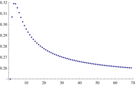
Figure 1: The first 70 values of $n(1/2-\mathbb{E}S_{n})$

3 Asymptotics of the length

We determine the asymptotic behavior of $\rho_{n}$, the radius of the $n$th segment.

Theorem 1.

We have the distributional convergence

$$n\left(\rho_{n}-\frac{1}{2}\right)\stackrel{{\scriptstyle{\mathcal{D}}}}{{\longrightarrow}}\mathrm{Exp}(4).$$

Accordingly, for any $k\geqslant 1$,

$$\lim_{n\to\infty}\mathbb{E}n^{k}\left(\rho_{n}-\frac{1}{2}\right)^{k}=\frac{k!}{4^{k}}\,.$$

Proof.

Since $\rho_{n}=1-S_{n}$, it is equivalent to prove the corresponding limit theorems for $1/2-S_{n}$.

It follows from (1) that

$$S_{n+1}=\begin{cases}S_{n}&\textrm{w.prob. $S_{n}/(1-S_{n})$}\\ \textrm{uniform on $[S_{n},1/2]$}&\textrm{w.prob. $(1-2S_{n})/(1-S_{n})$.}\end{cases}$$

Observe that given $S_{n}$, $S_{n+1}$ has the same distribution as $\max\{S_{n},U\}$, where $U$ is a uniform random variable on $[S_{n}/2,1/2]$, independent of $S_{n}$. Let $0\leqslant\alpha\leqslant 1/2$, and $U_{1}^{\alpha},U_{2}^{\alpha},\dots$ be independent, uniform random variables on $[1/4-\alpha/2,1/2]$. Define $M^{\alpha}_{n}=\max_{1\leqslant i\leqslant n}U^{\alpha}_{i}$. It is well-known in extreme value theory (Billingsley, 1995, p.192), and easy to check that

$$n\left(\frac{1}{2}-M_{n}^{\alpha}\right)\stackrel{{\scriptstyle{\mathcal{D}}}}{{\longrightarrow}}\mathrm{Exp}(4/(1+2\alpha)).$$ (6)

We say that $X$ stochastically dominates (or just dominates) $Y$ if $\mathbb{P}(X>x)\geqslant\mathbb{P}(Y>x)$ for all $x\in{\mathbb{R}}$.

To obtain a lower estimate, we use that $S_{n}\leqslant 1/2$, and thus an easy induction argument shows that $M^{0}_{n}$ dominates $S_{n}$. From this and (6) we obtain

$$\mathbb{P}\left(n\left(\frac{1}{2}-S_{n}\right)>x\right)\geqslant\mathbb{P}\left(n\left(\frac{1}{2}-M_{n}^{0}\right)>x\right)\to\mathrm{e}^{-4x},$$

i.e.

$$\liminf_{n\to\infty}\mathbb{P}\left(n\left(\frac{1}{2}-S_{n}\right)>x\right)\geqslant\mathrm{e}^{-4x},\quad x\geqslant 0.$$

The almost sure convergence $S_{n}\to 1/2$ heuristically means that with overwhelming probability, $1/2-S_{n}/2\approx 1/4$, hence for $n$ sufficiently large, $S_{n}$ behaves approximately like $M^{0}_{n}$ does. This heuristic idea is made precise as follows. Fix the small positive numbers $\beta>0$ and $\varepsilon>0$. Since $S_{n}\to 1/2$ a.s., for $n$ sufficiently large, $\mathbb{P}(S_{\beta n}<1/2-\varepsilon)\leqslant\varepsilon$. Moreover, if $S_{\beta n}\geqslant 1/2-\varepsilon$, then $S_{n}$ is minored by $M^{\varepsilon}_{n-\beta n}$. This can be shown again by induction. Thus, by (6),

$$\mathbb{P}\left(n\left(\frac{1}{2}-S_{n}\right)>x\right) =\mathbb{P}\left(S_{n}<\frac{1}{2}-\frac{x}{n}\right)$$

$$\leqslant\mathbb{P}\left(S_{n}<\frac{1}{2}-\frac{x}{n}\,\Big{|}\,S_{\beta n}\geqslant\frac{1}{2}-\varepsilon\right)+\varepsilon$$

$$\leqslant\mathbb{P}\left(M_{(1-\beta)n}^{\varepsilon}<\frac{1}{2}-\frac{x}{n}\right)+\varepsilon$$

$$\to\mathrm{e}^{-\frac{4x(1-\beta)}{1+2\varepsilon}}+\varepsilon\,,$$

i.e. for $x\geqslant 0$

$$\limsup_{n\to\infty}\mathbb{P}\left(n\left(\frac{1}{2}-S_{n}\right)>x\right)\leqslant\mathrm{e}^{-\frac{4x(1-\beta)}{1+2\varepsilon}}+\varepsilon.$$

Since $\varepsilon$ and $\beta$ are arbitrary, this gives the distributional convergence.

To prove the convergence of the moments, it is enough to show that for any $k\geqslant 1$, the sequence $\{n^{k}\left(\frac{1}{2}-S_{n}\right)^{k}\}_{n=1}^{\infty}$ is uniformly integrable (Billingsley, 1995, Theorem 25.12). The fact that $S_{n}$ dominates $M_{n}^{1/2}$ readily implies

$$\mathbb{P}\left(n\left(\frac{1}{2}-S_{n}\right)>x\right)\leqslant\mathrm{e}^{-2x},$$

which shows uniform integrability. ∎

In particular, $\mathbb{E}\rho_{n}=1/2-1/(4n)+o(n^{-1})$ and $\mathrm{Var}(\rho_{n})\sim 1/(16n^{2})$. The question of obtaining an exact or asymptotic formula for $\mathbb{E}S_{n}$ using only the recursive relations (4) and (5) remains open.

4 Limit distribution

In this section, we determine the limit behaviour of $Z_{n}$. Let $F(x)$ denote the cumulative distribution function of $Z$; based on the definition of $Z$, it follows that $F(x)=0$ if $x\leqslant-1/2$ and $F(x)=1$ if $x\geqslant 1/2$.

Theorem 2.

The distribution of $Z$ is a translated arcsine law: for $-1/2\leqslant x\leqslant 1/2$,

$$F(x)=\frac{2}{\pi}\arcsin\sqrt{x+1/2}\,.$$

Proof.

By (2), we have to determine the limit distribution of $\sum\varepsilon_{i}X_{i}$. Clearly, this is not affected by the steps where $X_{i}=0$. We introduce the thinned process $(\widetilde{Z}_{n},\tilde{\rho}_{n})$ as follows: for $n\geqslant 1$, let $\xi_{n}$ be independent Bernoulli(1/2) random variables, and $\widetilde{X}_{n}$ be a uniform random variable on $[0,1/2-\sum_{1}^{n-1}\widetilde{X}_{i}]$. The centre of the segment after the $n$th step of the thinned process is given by $\widetilde{Z}_{n}=\sum_{1}^{n}\xi_{i}\widetilde{X}_{i}$, and the radius is $\tilde{\rho}_{n}=1-\sum_{1}^{n}\widetilde{X}_{i}$. Plainly,

$$Z\stackrel{{\scriptstyle\mathcal{D}}}{{=}}\sum_{i=1}^{\infty}\xi_{i}\widetilde{X}_{i}.$$

Introduce $r_{n}=2\tilde{\rho}_{n}-1$. If $U_{1},U_{2},\dots$ are i.i.d. Uniform$(0,1)$ random variables, then setting $(\widetilde{Z}_{0},r_{0})=(0,1)$,

$$\begin{split}\widetilde{Z}_{n+1}&=\widetilde{Z}_{n}+\frac{1}{2}\,\xi_{n+1}(1-U_{n+1})r_{n}\,,\\ r_{n+1}&=U_{n+1}r_{n}\,.\end{split}$$ (7)

Notice that after choosing $(\widetilde{Z}_{1},r_{1})$, the process $(\widetilde{Z}_{2},r_{2}),(\widetilde{Z}_{3},r_{3}),\dots$ is a scaled and translated copy of the original one, which implies the distributional equation

$$Z\stackrel{{\scriptstyle\mathcal{D}}}{{=}}r_{1}\,Z^{\prime}+\widetilde{Z}_{1},$$ (8)

where $Z^{\prime}$ is independent from $(\widetilde{Z}_{1},r_{1})$, and has the same distribution as $Z$. Thus, for every $x\in[-1/2,1/2]$,

$$F(x) =\int_{0}^{1/2}F\left(\frac{x-y}{1-2y}\right)\,{\rm d}y+\int_{0}^{1/2}F\left(\frac{x+y}{1-2y}\right)\,{\rm d}y$$

$$=(1-2x)\int_{-\infty}^{x}\frac{F(z)}{(1-2z)^{2}}\,{\rm d}z+(1+2x)\int_{x}^{\infty}\frac{F(z)}{(1+2z)^{2}}\,{\rm d}z$$

$$=(1-2x)\int_{-1/2}^{x}\frac{F(z)}{(1-2z)^{2}}\,{\rm d}z+(1+2x)\int_{x}^{1/2}\frac{F(z)}{(1+2z)^{2}}\,{\rm d}z+\frac{1+2x}{4}\,.$$

This also shows that $F$ is continuously differentiable, and by differentiating we arrive at

$$F^{\prime}(x)=-2\int_{-1/2}^{x}\frac{F(z)}{(1-2z)^{2}}\,{\rm d}z+2\int_{x}^{1/2}\frac{F(z)}{(1+2z)^{2}}\,{\rm d}z+\frac{4xF(x)}{1-4x^{2}}+\frac{1}{2}\,.$$

Once again, we derive that $F$ is twice differentiable (being the reason for starting with the distribution function rather than the density function), whence

$$F^{\prime\prime}(x)=F^{\prime}(x)\frac{4x}{1-4x^{2}}\,.$$

Taking into account that $F^{\prime}(x)$ is a density function on $[-1/2,1/2]$ yields that the solution is

$$F^{\prime}(x)=\frac{1}{\pi\sqrt{(1/2+x)(1/2-x)}}\,,\,$$

the desired density function. ∎

5 Further remarks

Setting $v_{i}=U_{1}U_{2}\ldots U_{i}(1-U_{i+1})$, (7) implies that $\widetilde{Z}_{n}=1/2\,\sum_{0}^{n-1}v_{i}\xi_{i+1}$, hence the limit $Z$ has the infinite series representation

$$Z=\frac{1}{2}\sum_{i=0}^{\infty}v_{i}\xi_{i+1}.$$ (9)

It is easy to check that $\sum_{0}^{\infty}v_{i}=1$ almost surely, thus $v:=(v_{0},v_{1},\ldots)\in\Delta$, where

$$\Delta=\left\{x=(x_{0},x_{1},\ldots)\,:\,\sum_{i=0}^{\infty}x_{i}=1,x_{i}\geqslant 0,i=0,1,\ldots\right\}$$

is the infinite dimensional simplex. The construction of the random vector $v$ implies that it has the so-called GEM (Griffiths–Engen–McCloskey) distribution with parameter 1 (see the residual allocation model in Bertoin, 2006, p.89). This distribution appears in various contexts, such as prime factorisation of a random integer (Hirth, 1997); and in particular, the decreasing reordering of the GEM distribution is the so-called Poisson–Dirichlet distribution, which is one of the most important distributions in fragmentation theory, see Bertoin, 2006.

Using this terminology and (9), Theorem 2 can be reformulated as: if $v=(v_{0},v_{1},\ldots)$ is a GEM distributed random vector, and $\xi,\xi_{1},\xi_{2},\ldots$ is an iid sequence of Bernoulli random variables such that $\mathbb{P}(\xi=1)=1/2=\mathbb{P}(\xi=-1)$, which is independent of $v$, then $\sum_{i=0}^{\infty}v_{i}\xi_{i+1}$ has arcsine distribution. This theorem was first proved by Donnelly and Tavaré (1987), using the construction of the Poisson–Dirichlet distribution by means of an inhomogeneous Poisson process. Later Hirth (1997) also gave a proof by using the method of moments. As far as we know, our proof, solving an integral equation based on the distributional equality (8), is new.

Acknowledgements. Our thanks are due to Imre Bárány for introducing the problem to us and for illuminating discussions, and to Juan Carlos Pardo for bringing the connection with the Poisson–Dirichlet law to our attention. The authors are also grateful to the unknown referee for a number of comments and suggestions that improved the paper. While carrying out the research, the first named author held a pleasant visiting scholarship at the Isaac Newton Institute for Mathematical Sciences, University of Cambridge.

References

- [1] Bertoin, J. (2006) Random Fragmentation and Coagulation Processes, Cambridge University Press.
- [2] Billingsley, P. (1995) Probability and Measure, Wiley–Interscience Publication, New York.
- [3] Donnelly, P. and Tavaré, S. (1987) The population genealogy of the infinitely-many neutral alleles model. J. Math. Biol. 25, 381–391.
- [4] Hirth, U.M. (1997) Probabilistic number theory, the GEM/Poisson–Dirichlet distribution and the arc-sine law. Combinatorics, Probability and Computing 6, 57–77.
- [5] Tóth, B., Private communication, 2010.