Quantum Walk with Jumps

Abstract

We analyze a special class of $1$-D quantum walks (QWs) realized using optical multi-ports. We assume non-perfect multi-ports showing errors in the connectivity, i.e. with a small probability the multi-ports can connect not to their nearest neighbor but to another multi-port at a fixed distance – we call this a jump. We study two cases of QW with jumps where multiple displacements can emerge at one timestep. The first case assumes time-correlated jumps (static disorder). In the second case, we choose the positions of jumps randomly in time (dynamic disorder). The probability distributions of position of the QW walker in both instances differ significantly: dynamic disorder leads to a Gaussian-like distribution, while for static disorder we find two distinct behaviors depending on the parity of jump size. In the case of even-sized jumps, the distribution exhibits a three-peak profile around the position of the initial excitation, whereas the probability distribution in the odd case follows a Laplace-like discrete distribution modulated by additional (exponential) peaks for long times. Finally, our numerical results indicate that by an appropriate mapping a universal functional behavior of the variance of the long-time probability distribution can be revealed with respect to the scaled average of jump size.

1 Introduction

The quantum walk (QW) is a quantum mechanical model, a generalization of a classical random walk. It was introduced in 1993 aharonov-1993-48 ; gudder-1988 ; grossing-1988 and later found fruitful applications as a tool to design efficient quantum algorithms. The model of a quantum walk was defined in two distinct ways: continuous- and discrete-time. In the former, the particles (walkers) are achiral, the Hilbert space is spanned by the discrete position states corresponding to vertices of a graph. In the discrete-time case, the introduction of chirality is unavoidable. The Hilbert space corresponding to the chirality has its dimension equal to the number of possible directions of a step.

A possible experimental implementation of a classical random walk is the Galton board (also known as Quincunx). Here a large number of balls (walkers) fall through the board, changing their direction randomly on periodically arranged pins and forming so a binomial distribution of their final position. A quantum analogy of the Galton board (and one possible implementation of the QW) is shown in Fig. 1 where the walker is a coherent light pulse moving through a medium with periodical boundaries that split the signal; finally, there are detectors at the end which represent the quantum equivalent of the bins in the classical model.

The spectrum of investigation of the QW (and its modifications) is broad. The original idea was presented in aharonov-1993-48 ; gudder-1988 ; grossing-1988 and since then a few review papers have been published kempe-2003-44 ; meyer96from ; Vanegas-Andraca-2008 . Recently, there have been studies of QW allowing Lévy noise in the model. The latter is introduced via randomly performed measurements with waiting times following a Lévy distribution romanelli-2007-76 ; romanelli-2007-75 . The most relevant paper for the present work is yin-2007 in which the properties of the one-dimensional continuous-time QW in a medium with static and dynamic disorder are examined. Other studies of the QW have focused on the meeting problem of two particles stefanak-2006-39 ; stefanak-2009-11 . Recurrence properties of the walker have been investigated in stefanak-2009-11 ; Stefanak-2008 ; stefanak-2008-78 . Moreover, localization of the walker has been studied in konno-2009-3 . Finally, a theoretical investigation of the QW in random environment has been performed in konno-2009-4 ; konno-2009-1 , where a robust mathematical definition of a random environment is provided.

The simplest analytic task in the study of quantum walks is to determine the functional expression of the probability to find a particle at a certain location at a certain time. General analytic calculations of quantum walks are not known. However, asymptotic solutions of several quantum walk models have been found using path integral techniques in konno-2009-3 ; konno-2009-4 ; konno-2009-1 ; konno-2002 ; konno-2008-1 ; konno-2008-2 ; konno-2009-2 ; konno-2005-1 ; konno-2005-2 and in stefanak-2006-39 ; stefanak-2009-11 using Fourier transform.

Since their introduction, many experimental groups have tried to implement quantum walks. A number of successful realizations of one-dimensional QW have been reported in optical lattices Dur-2002 , trapped ions Travaglione-2002 , and cavity QED Sanders-2003 . More recently, additional realizations of a quantum walk using atoms in an optical lattice Karski-2009 , trapped ions Schmitz-2009 ; Zahringer-2010 and photons Schreiber-2010 have been announced.

Recent studies of quantum systems ElGhafar-1997 ; Kim-2000 with random potentials have shown that localization of the particle can occur as a result of the randomness. Focusing on quantum walks, Ribeiro et al. Ribeiro_2004 have used two different coin operators switched according to the Fibonacci series and they have observed localization in the system. Yin et al. yin-2007 have numerically simulated the continuous-time QW on a line and they have observed Anderson localization only in the case of static disorder, while dynamic disorder leads to decoherence and a Gaussian position distribution. In addition, effects of spatial errors have been studied by Leung et al. in Leung-2010 . They have examined QWs in $1$ and $2$ dimensions on networks with percolation where the missing edges or vertices absorb the walker, leading to topological randomness of the graph.

The simplest discrete QW is described by the action of the coin and the step operator. Much attention was paid to the alternation of the coin operator – position or time dependent coin and its implications on the walker dynamics have been extensively discussed. However, little focus was given to changes of the step operator. Our analysis takes a step in this direction. While assuming a constant coin we study changes in the step operator. When assuming a Galton board realization this amounts to a change in the connectivity between the layers of beam splitters forming the walks.

In the present paper, we focus on the QWs where signals can jump to a distant location, which is a generalization motivated by Lévy flights in classical mechanics. The jump may be caused by an inhomogeneity of the material, spatial proximity of non-neighbor channels or scrambling in the topology of the network (for instance relabeling of input-output label of multiports forming the network realising the QW).

We study two basic modifications of the QW. In the first case, which we call dynamic disorder, the jumps are prepared as independent and identically distributed in time, whereas in the second case, called static disorder, the positions of the jumps are perfectly correlated. We investigate the problem using computer simulations employing the Zarja library Lavicka-2010 and its offspring library focused on the QW .

The structure of the article is as follows. In Section 2, we motivate our study from an experimental point of view. Then we define a model with next neighbor interactions only. In Section 3, we show the results of the simulations based on Monte Carlo method. In Section 4, we discuss our results and draw conclusions. Finally, we describe in the appendix the set of operators used in the simulations and an algorithm to sample from the appropriate probability distribution.

2 Definition of a Quantum Walk

We model a sequence of optical layers by an array of multi-ports, or beam splitters (Fig. 2), forming so a large interferometer, see Fig. 1 – this is a quantum analog to Galton’s board (Quincunx). Due to the regular structure of the interferometer, it is natural to treat the temporal evolution of the system in discrete steps, discretized by the time needed for an excitation to travel the distance between two consecutive layers at a constant angle. If we let this angle approach the right angle, we obtain so-called static disorder (see Fig. 3d,e), where the same set of beam splitters is used repeatedly in every time step. An excitation enters the system of multi-ports at one selected position and spreads due to the coherent interaction with the beam splitters. A number of detectors is placed in the interferometer so that the signal hits one detector in every possible path after a given number of interactions with the medium. The resulting scheme is an implementation of the QW.

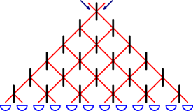
Figure 1: A schematic of an interferometer simulating material and implementing a random walk. The red lines are the connections of multi-ports along which the signal is transmitted. The light blue half-circles represent detectors. The blue arrows are two selected input channels. Every horizontal layer of the multi-ports is accessed simultaneously.

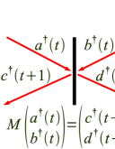
Figure 2: Action of a beam splitter on the input states $a^{\dagger}(t)$ and $b^{\dagger}(t)$ which are transformed to the output states $c^{\dagger}(t+1)$ and $d^{\dagger}(t+1)$ using the matrix $M$.

In the following, we introduce two ways to describe the system. First we introduce the standard notation for a discrete-time QW. We define the basis states of the system as states localized at the beam splitters just before or after the interaction takes place. Therefore, every basis state is described by a position within the beam splitter layer (an integer number) and a chirality, which can take values $L$ or $R$ for left and right, respectively. Formally, we define the state space $\mathcal{H}$ of the system as

$$\mathcal{H}=\mathcal{H}_{S}\otimes\mathcal{H}_{C}$$ (1)

where a “position” space $\mathcal{H}_{S}$ and a “coin” space $\mathcal{H}_{C}$ (the name stemming from the idea of a random walker tossing a coin to decide the direction of his next step) are defined as

$$\mathcal{H}_{S}=\text{Span}\{|n\rangle\mid n\in\mathbb{Z}\}$$ (2)

and

$$\mathcal{H}_{C}=\text{Span}\{|L\rangle,|R\rangle\}.$$ (3)

We define all the numbered states $|n\rangle$, as well as the states $|L\rangle$ and $|R\rangle$, to be normalized and mutually orthogonal. Therefore, $\mathcal{H}_{S}$ is isomorphic to the space $\ell^{2}$ of quadratically integrable complex sequences and $\mathcal{H}_{C}$ to $\mathbb{C}^{2}$. The basis states are then constructed as tensor product basis states $|n,R\rangle$ and $|n,L\rangle$, where $n\in\mathbb{Z}$.

Following Konno konno-2009-1 , we define that the state of the system at time $t$ in a random environment $\omega$ is described by the positive semi-definite density matrix $\widehat{\rho}_{\omega}(t)$ on $\mathcal{H}$ having $\mathbf{Tr}\ \widehat{\rho}_{\omega}(t)=1$. Thus the density matrix of the system $\widehat{\rho}(t)$ at time $t$ is

$$\widehat{\rho}(t)=\int_{\omega\in\Omega}\widehat{\rho}_{\omega}(t)\cdot\mathbb{P}(d\omega),$$ (4)

where symbols $\Omega$ and $\mathbb{P}$ will be specified later in section 2.2.

The evolution of the system by one timestep from $t$ to $t+1$ for one particular setup of environment $\omega$ is described by a unitary operator $U_{\omega}(t\rightarrow t+1)$ which acts as follows:

$$\widehat{\rho}_{\omega}(t+1)=U_{\omega}(t\rightarrow t+1)\cdot\widehat{\rho}_{\omega}(t)\cdot U_{\omega}^{{\dagger}}(t\rightarrow t+1)$$ (5)

just the same way as typical propagator on density matrix in quantum mechanics in, e.g., Blank_1993 .

2.1 Quantum Walk

The QW described, e.g., in kempe-2003-44 assumes that the conditions of the environment are stable and thus it holds $\widehat{\rho}(t)=\widehat{\rho}_{\omega}(t)$ for all $\omega\in\Omega$. If we set up the initial density matrix $\widehat{\rho}(0)$ as a pure state $|\psi_{0}\rangle\in{\cal H}$ using $\widehat{\rho}(0)=|\psi_{0}\rangle\langle\psi_{0}|$, then the system is in a pure state $|\psi_{T}\rangle=\prod_{t=0}^{T-1}$ $U^{QW}(t\rightarrow t+1)|\psi_{0}\rangle$ (the product expanded in the proper time ordering) at every timestep $T$ and the appropriate density matrix is $\widehat{\rho}(T)=|\psi_{T}\rangle\langle\psi_{T}|$. Moreover, the original QW was defined with fixed unitary operator $U^{QW}(t\rightarrow t+1)$ in the form of a composition of two unitary operations as follows:

$$U^{QW}(t\rightarrow t+1)=S\cdot C.$$ (6)

Thus, the evolution of the walker at time $T$ is $|\psi_{T}\rangle=$ $\left(U^{QW}\right)^{T}|\psi_{0}\rangle$. The operator $C$ is called a coin operator and describes the transformation induced by a beam splitter. Here the position of a localized state stays unchanged and the operation acts only on the coin state as $C=I\otimes M$, where $M$ is a unitary operation transforming the probability amplitudes due to a partial reflection on the beam splitter. We assume for simplicity that all the beam splitters have the same physical properties and perform a Hadamard transform on the input states,

$$M=\frac{1}{\sqrt{2}}\left(\begin{matrix}1&\phantom{-}1\\ 1&-1\end{matrix}\right).$$ (7)

The operator $S$ represents the propagation of an excitation in the free space between the beam splitters. Hence, the chirality of a basis state does not change but the position is shifted by $\pm 1$, depending on the coin state. We can express $S$ as

$$S=\sum_{n\in\mathbb{Z}}(|n+1,R\rangle\langle n,L|+|n-1,L\rangle\langle n,R|).$$ (8)

It is easy to show that the sum converges and defines a unitary operator defined on all the state space $\mathcal{H}$.

If the initial state of the walker is one of the basis states, for example $|0,R\rangle$, it evolves under the operation $U$ so that in terms of a complete measurement in the position space, the probability spreads to both sides from the starting position. However, it is bounded between the positions $-t$ and $t$ as it can’t change by more than $1$ in either direction in any step. Moreover, due to the fact that a transition by $1$ has to be done in every time step, the walk is restricted at each time $t$ to a subspace spanned by the basis states for which the position shares the same parity with $t$.

Alternatively, we can describe the path of the walk in terms of the edges of the underlying graph instead of its vertices, following the physical trajectories of the excitation and eliminating the need to describe the propagation between beam-splitters. In the following, we will call these edges “channels”. Due to the fact that every channel lies in between two consecutive positions of the beam splitters, as well as to avoid confusion in the notation, we will denote the channels by half-integer numbers. A notation based on the channel formalism can be introduced and mapped to the previously defined state space in more ways. One such possibility is to identify the channel as a given time $t$ with the state in which the excitation is at the end of the propagation, just before hitting another beam splitter (or a detector). This time-dependent mapping is given by the formulas

$$|n+{\textstyle\frac{1}{2}};t\rangle=\begin{cases}|n,L\rangle&\text{if $t$ is even},\\ |n+1,R\rangle&\text{if $t$ is odd}\end{cases}$$ (9)

for even $n$ and

$$|n+{\textstyle\frac{1}{2}};t\rangle=\begin{cases}|n+1,R\rangle&\text{if $t$ is even},\\ |n,L\rangle&\text{if $t$ is odd}\end{cases}$$ (10)

for odd $n$. One can verify that such a mapping respects the parity rule and covers all the subspace of $\mathcal{H}$ that is actually used by the quantum walk if we assume that the initial state was $|0,R\rangle$ or $|0,L\rangle$. In particular, these two initial states are denoted $|-{\textstyle\frac{1}{2}};0\rangle$ and $|{\textstyle\frac{1}{2}};0\rangle$ in the channel notation, respectively; cf. Fig. 1 for a visualization. Since the instantaneous chirality of an excitation is uniquely given by the position of the channel and the time, we do not need to specify the coin degree of freedom explicitly in this approach. The “coin toss” and “step” are merged into one unitary operation which mixes neighboring channels in pairs.

The above discussion gives two equivalent ways to describe QW on a line. Throughout this work, we will use the latter approach as it makes it much simpler to describe the jumps in the network.

2.2 Quantum Walk with jumps

We will assume that the quantum walk is disturbed by random topological errors, see Fig. 3, which are modeled by random changes of connectivities between the multi-ports forming the network in Fig. 1. We focus our analysis on two distinct situations. First we will assume that we deal with the repetition of random but stationary errors. Stationary errors mean that in each layer the same jumps appear. One could also realize static disorder with a single set of beam splitters, if the incident beam is parallel to the layer of beam splitters and repeatedly sent through them (see Fig. 3d,e). The other situation refers to the case when in each layer jumps are generated independently. We refer to the latter situation as dynamic disorder (see Fig. 3a,b,c).

In the QW with jumps we assume that the unitary operators $U_{\omega}(t\rightarrow t+1)=U_{\omega}^{jump}(t\rightarrow t+1)$ in Eq. 5 are random (the set of such operators forming a probability space of random unitary operators) and that $U_{\omega}^{jump}(t\rightarrow t+1)$ can be written in form of a joint action of two unitary operations,

$$U_{\omega}^{jump}(t\rightarrow t+1)=S_{\omega}^{jump}(t)\cdot U_{\omega}^{QW}(t\rightarrow t+1),$$ (11)

where $U_{\omega}^{QW}(t\rightarrow t+1)$ is the evolution operator of the $1$D QW in a clean media without errors, defined by Eq. 6.

We define that the set of all unitary operators $S_{\omega}^{jump}(t)$ forms the probability space $S(\Omega,{\cal F},\mathbb{P})$. For the sake of simplicity of the following discussion and the numerical simulations, we make the set $\Omega$ finite by replacing the infinite walking space by a cycle of size $N$ with a periodic boundary condition. If $N$ is chosen sufficiently large, this imposes no restriction on the validity of the results. The sample space $\Omega$ is then the set of all the possible combinations of jump operators $\mathbf{{P}}_{j_{i}}$ exchanging signals in channels $j_{i}$ and $j_{i}+j$, having the matrix form

$$\mathbf{{P}}_{j_{i}}=\left(\begin{smallmatrix}1&0&\ldots&0&\ldots&0&\dots&0&0\\ 0&1&\ldots&0&\ldots&0&\dots&0&0\\ \vdots&&\ddots&&&&&&\vdots\\ 0&0&\ldots&0&\ldots&1&\dots&0&0\\ \vdots&&&&\ddots&&&&\vdots\\ 0&0&\ldots&1&\ldots&0&\dots&0&0\\ \vdots&&&&&&\ddots&&\vdots\\ 0&0&\ldots&0&\ldots&0&\dots&1&0\\ 0&0&\ldots&0&\ldots&0&\dots&0&1\end{smallmatrix}\right),$$ (12)

i.e., that of a transposition operator. ${\cal F}=2^{\Omega}$ is the $\sigma$-field defined on

$$\Omega=\left\{\mathbf{E},\mathbf{P}_{j_{1}},\mathbf{P}_{j_{1}}\mathbf{P}_{j_{2}},\ldots\right\}$$ (13)

and $\mathbb{P}:{\cal F}\rightarrow\left[0,1\right]$ is the probability measure, specified by the probability of elementary events, defined as

$$\mathbb{P}\left(\pi\right)=\frac{1}{Z}p^{tr(\pi)}\left(1-p\right)^{N-2\cdot tr(\pi)}.$$ (14)

We define $tr(\pi)$ as the number of transpositions of indexes forming permutation $\pi$, $N$ is equal to the size of the system and consequently to the dimension of jump operators $\mathbf{{P}}_{j_{i}}$, $p$ is probability that one pair of errors with distance $j$ occurs and finally $Z=\left(1+\left(-p\right)^{\frac{N}{g}}\right)^{g}$ is normalization where $g=\mathrm{gcd}(N,j)$ ($\mathrm{gcd}$ stands for greatest common denominator).

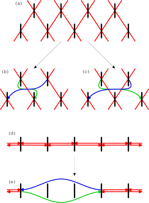
Figure 3: Schematic picture of different jumps of the signal. Scheme (a) shows a part of interferometer without jumps. Two schemes in the middle, namely (b) and (c), show dynamic disorder pattern where (b) and (c) shows even ($j=2$) and odd ($j=3$) size of jump, respectively, which can emerge independently at every level. Scheme (d) shows an interferometer without jumps for static disorder and a jump of size $j=2$ is illustrated in scheme (e).

3 Simulation of the model

The disorder of the system is expressed by the set of unitary operators displacing the signal to a distant location. In general, the system can undergo either static or dynamic disorder. The system with static disorder is propagated by random unitary operators fixed during the realization, i.e., the operators are correlated in time. On the other hand, the evolution of the system undergoing dynamic disorder is governed by the operators that are independently and identically distributed in time.

3.1 Static disorder

The random unitary operators propagating the system with typical structure of jumps according to Eq. 12 can have due to mapping 9 and 10 one of two fundamental distinguished forms, according to the parity of the length of the jumps induces by the errors in the media. Jumps of even lengths $j$ do not change chiral state of the walker in Hilbert state ${\cal H}$ in contrast to jumps of odd lengths $j$ which swap chirality of the walker from state $L$ to $R$ and vice versa.

3.1.1 Odd jumps

The only tunable parameter that affects the evolution of the walker is the probability $p$ that one error (jump with distance $j$) occurs. The value of the parameter $p$ close to $0$ should produce typical chiral $1$D QW pattern, which is clearly visible on the top of Fig. 4. Here the QW was initiated in a localized state $|0+{\textstyle\frac{1}{2}};0\rangle$ of the walker, causing an asymmetrically distributed walk. Higher values of $p$ produce totally different pattern where high-frequency oscillations of probability distribution of positions of the walker are suppressed. In the middle and at the bottom of Fig. 4 the probability distribution of the positions of the walker shows Laplace distribution modulated by Laplace distributed peaks with distance $j$ between neighboring peaks (clearly observable as the small triangular peaks modulated on a bigger structure in Fig. 4).

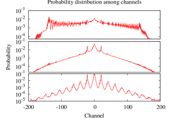
Figure 4: Typical patterns of probability distribution of position of the walker among channels after $T=200$ steps for $j=21$, from the top to the bottom $p=0.01$, $p=0.05$ and $p=0.2$. On the top, the typical structure of the QW without jumps that is perturbed by formation of an extra central peak. In the middle, we see formation of Laplace-like tail and $3$ peaks with distance $j$. Central peak is located at the position of the initial excitation of the system at $T=0$. On the bottom, the whole distribution follows an overall exponential decay which is modulated by exponential peaks with a distance $j=21$ between maxima. The graphs were obtained using Monte Carlo method after $R=20000$ runs of the randomized evolution.

Previous observations of the fundamental change induced by the variation of $p$ is supported by Fig. 5 showing evolution of the probability distribution. The top part shows the typical structure of evolution of the probability distribution of the walker—the quantum carpet Berry-2001 —with additional quantum carpets on the border of the main one which were formed at initial stages of evolution. For small values of $p$, the interference is not strong enough to change the pattern of distribution. In contrast, in the second case displayed at the bottom of Fig. 5, where $p=0.5$, we observe a typical structure of equidistant peaks separated by valleys of width $j$. The peaks are formed early during evolution and they do not change their positions later.

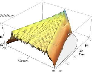
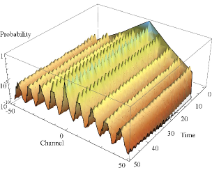
Figure 5: Probability distribution among channels for $T=200$, $R=20000$ and $j=11$; from the top to the bottom $p=0.01$ and $p=0.5$. On the top, the maxima of probability move outward similarly to the standard case of the QW. On the bottom, the maxima are formed and they stay at the point of original formation.

To support the idea that the walker froze in the close neighborhood of a few preferred locations we analyzed the evolution of entropy and variance of the probability distribution of the position of the walker. The evolution of the variance, shown in Fig. 6, visualizes the observation from the previous paragraph. For a probability $p$ close to $0$ (unperturbed QW), we see a clear ballistic diffusion of the walker ($\sigma^{2}\sim t^{2}$)—in contrast to this we stress that for a classical random walker $\sigma^{2}\sim t$. Increasing $p$, we observe sub-ballistic diffusion and finally, in the range close to $1/2$, the variance tends to finite constant.

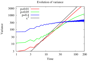
Figure 6: Evolution of variance of the system f or $T=200$, $R=20000$ and $j=11$. Transition from the case of ballistic diffusion of the signal for probabilities $p$ close to $0$ to the case of sub-ballistic diffusion, demonstrated for $p=0.05$ can be observed, and finally we observe for $p=0.4$ that variance tends to a constant, i.e., diffusion coefficient approaches $0$ and the walker ceases to “spread”—a characteristic property of localization anderson-1958 .

Next, we turn our attention to the evolution of the classical (Shannon) entropy of the probability distribution of the positions of the walker, which is shown in Fig. 7. The evolution of the classical entropy follows an analogous behaviour as described in the case of variance in the previous paragraph. Thus, we can observe for the probability $p$ close to unperturbed QW an increase of classical entropy proportional to $\ln\left(t\right)$. However, rising probability $p$ causes slower and slower increase in entropy in time and for the case $p=0.4$ we observe a saturation of entropy.

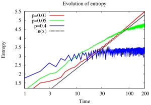
Figure 7: Evolution of classical (Shannon) entropy of probability distribution of positions of walker for $T=200$, $R=20000$ and $j=11$. Classical entropy is a rising function of time $t$ for $p=0.01$ where the functional form is proportional to $\ln t$. On the other hand, increasing probability $p$ causes “freezing” of the evolution, as can be observed for $p=0.4$.

The conclusion of the above paragraphs on odd-sized jumps in the QW is that we clearly observe localization of quantum walker in static disorder media described by the probability space of random unitary operators $S(\Omega,{\cal F},P)$ parametrized by probability $p$. Moreover, the numerical results suggest that taking separately odd and even timesteps the probability distribution of the position of the walker converges to a stationary distribution:

$$\langle{n+\frac{1}{2};2t}|\widehat{\rho}(2t)|{n+\frac{1}{2};2t}\rangle\xrightarrow{t\rightarrow+\infty}\mathbb{P}_{p,j}^{even}\left(n+\frac{1}{2}\right)$$ (15)

$$\langle{n+\frac{1}{2};2t+1}|\widehat{\rho}(2t+1)|{n+\frac{1}{2};2t+1}\rangle\xrightarrow{t\rightarrow+\infty}$$

$$\mathbb{P}_{p,j}^{odd}\left(n+\frac{1}{2}\right).$$ (16)

$\mathbb{P}_{p,j}^{even}(n$ ${}+\frac{1}{2})$ and $\mathbb{P}_{p,j}^{odd}(n+\frac{1}{2})$ are universal distributions for odd and even timesteps for probabilities $p$ in range close to $\frac{1}{2}$ and the size of the region of convergence is also dependent on $j$.

Let us consider the fundamental properties of the asymptotic probability distribution $\mathbb{P}_{p,j}^{even}\left(n+\frac{1}{2}\right)$; variables of the probability distribution $\mathbb{P}_{p,j}^{odd}\left(n+\frac{1}{2}\right)$ for odd timesteps are different but general properties are shared. We concluded from Fig. 4 that we observe a formation of an overall Laplace distribution modulated by Laplace distribution of peaks, both in the form

$$\mathbb{P}\left(x\right)=C\exp\left(-\frac{|x-\mu|}{a}\right),$$ (17)

where $\mu$ is the mean value of the distribution and $a$ is related to variance via $Var\ \mathbb{P}\left(x\right)=2\cdot a^{2}$. Our aim is to estimate the inverse parameter $\frac{1}{a}$ of Laplace distribution in two cases for

• the whole distribution (with mean at the point of injection),

• the modulated peaks (with mean at the center of the peak).

We focus on the shape of the whole probability distribution. The plots in Fig. 8 suggest a U-shape function of the fitted inverse parameter $1/a$ of the Laplace distribution for all parameter values. We vary the probability $p$ and we connect points for the same jump sizes $j$. Defining the $x$-axis as $x=p\cdot j$ we put all minima at a fixed position. Thus, for the minima $p\cdot j=x_{min}$ holds where an approximation of the constant is $x_{min}=2$. The values of minima of the fitted inverse parameter $1/a$, reached for $p=x_{min}/j$, form an increasing function of jump size $j$.

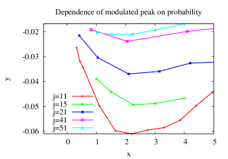
Figure 8: Fit of the inverse parameter $\frac{1}{a}$ of the probability distribution of position of the walker for $T=200$ and $R=15000$ with various odd sizes of jump $j$ taking $x$-axis as $x=p\cdot j$ and $y=1/a$. We observe the formation of a U-shape function for constant sizes of jump $j$ and changing $x=p\cdot j$ with a minimum at $x_{min}=2$.

The size of the central peak is $j$, $j/2$ on the left and on the right from the maximum at $0$. Estimation of the inverse parameter $1/a$ of the central peak is shown in Fig. 9. The shape of the central peak is an increasing linear function of probability of jump $p$ independent of the size of jump $j$. Thus the central peak becomes steeper and steeper with increasing $p$—localization of the walker becomes more evident. This is true not only for the central peak but it holds true for the other peaks as well, see Fig. 4.

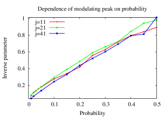
Figure 9: Fit of the inverse parameter $\frac{1}{a}$ of the central peak of the probability distribution of the position of the walker for $T=200$ and $R=15000$ with various odd sizes of jump $j$. Increasing probability causes linear increase of the inverse parameter $\frac{1}{a}$ with $p$ when $j$ is fixed. Moreover we observe a universal dependence on $p$, independent of the length of jump $j$.

Let us look at the dependence of entropy of probability distribution $\mathbb{P}_{j,p}\left(n+\frac{1}{2}\right)$ to find a walker at position $n+\frac{1}{2}$. We plot it in Fig. 10 where the entropy was measured by both extensive and non-extensive measures. In the first case, the extensive measure is classical (Shannon) entropy. The non-extensive one is the $q$-entropy introduced by Tsallis, which for a particular $q=1$ reduces to the classical entropy (for more about $q$-statistics, see Tsallis-1988 ; Tsallis-2004 ; Tsallis-2009a ; Tsallis-2009b ; Tsallis-2009c ). Both entropies are decreasing functions for increasing disorder measured by $p$. This leads to a counter-intuitive statement that increasing classical disorder organizes quantum system even if measured by a non-extensive entropy (in classical random walk longer jump causes increasing variance and increasing entropy as well). Moreover, the $q$-entropy of the probability distribution of position of the walker for the parameter value $q=2$ brings all curves corresponding to different sizes of jump $j$ on one single curve. This means that if we take into account non-additivity of the system quantified by the parameter $|1-q|$ (taken form the theory of the nonadditive $q$-entropy), we can map the QWs between each other for different sizes of error $j$ holding probability of occurrence of pair of error positions $p$ constant for $q=2$.

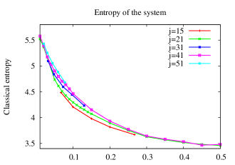
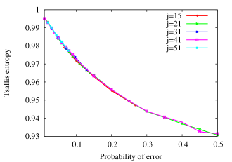
Figure 10: Classical entropy of the probability distribution is on the top, Tsallis entropy for $q=2$ on the bottom for parameters set to $T=200$ and $R=15000$. Classical entropy, on the top, decreases for increasing $p$ but the shape of the dependence is different for different values of $j$. The shape of the decrease becomes the same for Tsallis entropy with parameter $q=2$ as seen on the bottom.

Finally, the last studied variable for the QW with static disorder was the variance of position displacements $Var\ \mathbb{P}_{p,j}$, plotted in Fig. 11 on the left and with rescaled axes on right-hand side. The variance forms a U-shaped function of $p$ with moving minima for different but fixed $j$. Rescaling the axis $x=p\cdot j^{\alpha}$ where $\alpha=1.04$ and axis $y=j^{-\beta}\cdot Var\ \mathbb{P}_{p,j}$ where $\beta=1.67$, we clearly see from Fig. 11, right inset, that there is a universal U-shape function $f_{\mathbf{odd}}^{*}$(x) fulfilling

$$f_{\mathbf{odd}}^{*}\left(x\right)=j^{-\beta}\cdot Var\ \mathbb{P}_{x,j}.$$ (18)

Due to relation $\alpha\simeq 1$ and the U-shape of function $f_{\mathbf{odd}}^{*}\left(x\right)$ we can conclude that the overall variance of probability distribution of the walker’s position is strongly correlated with the fit of the inverse parameter $1/a$ (of the Laplace distribution) of whole probability distribution.

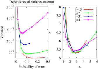
Figure 11: Dependence of variance of the probability distribution for odd $j$ on $p$ for $T=200$ and $R=15000$ is shown. The typical U-shape function can be observed with shifted position of the minimum. On the right, there are the same data with rescaled $x$-axis where $x=p\cdot j^{\alpha}$ where $\alpha=1.04$ and $y$-axis where $y=j^{-\beta}Var(i)$ where $\beta=1.67$. The data fit on the same U-shape function reaching their minimum at the same place.

3.1.2 Even jumps

Let us now assume that the ensemble of the random unitary matrices is still parametrized by the probability $p$ that the pair of erroneous positions occur, but the distance of a pair of errors $j$ is an even number and due to the mappings 9 and 10 the chirality of walker does not change. The typical formation of Laplace-like distribution as in the case of odd jumps is not present, but instead we observe a $3$-peaked structure, as seen in Fig. 12 (left-right asymmetric due to the initial condition) modulated by a periodic function that has its period equal to the length of jump $j$. To emphasize the difference between odd and even $j$, we conclude that both cases form a located peak at the initial position of the walker. However, odd sized jumps $j$ cause Laplace-like overall distribution while the case of even $j$ can form a $3$-peaked distribution where the central (localized) peak is sharp but the two others are broad and peaks with distance $j$ are modulated on the overall structure.

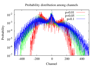
Figure 12: Probability distribution among channels for $T=200$ and $R=15000$ in the case of even sized jumps ($j=20$). The probability distribution forms a $3$-peak structure that is modulated by additional periodical small peaks which are separated by $j$.

3.2 Dynamic disorder

The static disorder analyzed in the preceding sections assumes random, but time-correlated emergence of pairs of errors that are expressed in the set of random unitary operators $S(\Omega,{\cal F},\mathbb{P})$. In contrast, dynamic disorder assumes independent and identically distributed random unitary operators from the same probability space $S(\Omega,{\cal F},\mathbb{P})$.

Let us consider on the probability distribution of the position of the walker, plotted in Fig. 13 on the top. We observe decoherence of the quantum walker forming a distribution reminiscent of a Gaussian distribution modulated by $1$D QW patterns for small probabilities of jump $p$. On the other hand, large $p$ causes a modulation by valleys with distance $j$ between peaks. The functional dependence of the standard deviation of the probability distribution of position of the walker on probability of jump $p$ in Fig. 13 on the bottom shows a linear behavior.

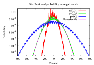
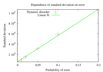
Figure 13: On top, probability distribution among the channels for dynamic disorder for $T=100$, $R=5000$ and $j=40$. Probability distribution can be fitted to a normal distribution where residual patterns of the QW are present for $p=0.01$; for $p=0.2$, formation of periodical valleys modulated on overall distribution (similar to static disorder with an odd size of jump) can be observed. On the bottom, functional dependence of standard deviation of the probability distribution of the position of the walker on probability of error $p$ and its linear fit.

4 Discussion and Conclusions

We have defined a modification of the QW in $1$D where the environment causes long but fixed-size jumps that emerge with a constant probability—the model is no longer deterministic but stochastic, depending on a random variable. In one step, first a unitary QW coin and shift operator act on the state, then a stochastic displacement operator generates jumps. We have studied two classes of QW with disordered connections between beam-splitters. First, dynamic disorder model shows decoherence that leads to Gaussian distribution modulated by residual patterns of QW (for small probabilities of jump $p$) or by valleys (for large probabilities of jump $p$). The standard deviation of the position of the walker is a linear function of $p$. In the second case, the QW is perturbed by static disorder. The behaviour of the model depends on the size of jump and we have investigated odd and even jump sizes separately. Even jump sizes cause localization of the walker at the initial position and two other broad peaks modulated by oscillations with a period of the size of jump $j$. The focus of the paper, however, was mainly given to jumps with odd size. In this case, the evolution of the variance shows a transition from the ballistic diffusion to a no-diffusion regime with increasing $p$ and this observation is supported by numerical calculation of classical entropy which changes from logarithmically increasing regime to a no-growth regime.

In addition, the probability distribution of positions of the walker changes from a pattern typical to the QW to Laplace distribution modulated by Laplace distributed peaks separated by the size of jump $j$. The formation of Laplace distribution depends on the probability $p$ that a pair of errors occurs. Moreover, the model exhibits the unusual property that classical disorder in quantum system can decrease, i.e., we observe a decrease of both the classical (Shannon) and $q$-entropy (with $q=2$) of measurements. Finally, our numerical calculation shows that using non-additive $q$-entropy with $q=2$ there is an universal functional dependence of $q$-entropy on $p$ for arbitrary $j$. The next part of out investigation was turned to the variance of the probability distribution. Our numerical results indicate that there is an universal functional form of variance of the probability distribution of the position of the walker—variance multiplied by $j^{-\beta}$ is an universal U-shaped function of one variable $p\cdot j^{\alpha}$ where $\alpha=1.04$ and $\beta=1.67$. The functional dependence of the universal function shows a minimum which separates two regimes—one with decreasing variance and the second with increasing variance. To put this result in the broader context of Complex Systems and Game Theory, we note that similar behavior of variance of attendance has been observed in Minority Game, exhibiting dynamical phase transition, see, e.g., Lavicka-2010 ; challet-1998 .

5 Acknowledgements

The financial support by MSM 6840770039, MŠMT LC 06002, GAČR 202/08/H072, the Czech-Hungarian cooperation project (KONTAKT CZ-11/2009), Hungarian Scientific Research Fund (OTKA) under Contract No. K83858, the Emmy Noether Program of the DFG (contract No LU1382/1-1) and the cluster of excellence Nanosystems Initiative Munich (NIM) is gratefully acknowledged.

Appendix A Properties of the set of operators

Let the unperturbed walking space be represented by a cycle graph with $N$ vertices where every vertex represents a channel in the main text. The errors in the network are represented by swapping the walker’s probability amplitudes between vertices labelled $i$ and $i+j\bmod N$ for a fixed $j$, which happens with a relative probability $p$. With a relative probability $1-p$, a vertex is left intact. Finally, a vertex already exchanged with another one cannot be used for another transposition in the same permutation.

These conditions give the probability of a permutation $\pi$ in the form

$$\mathbb{P}(\pi)=\frac{1}{Z^{(N)}}p^{tr(\pi)}(1-p)^{N-2\cdot tr(\pi)},$$ (19)

where $tr(\pi)$ denotes the unique number of independent transpositions forming the permutation $\pi$. A factor of $2$ in the exponent of $1-p$ is present due to the fact that every transposition reduces the number of unused vertices by $2$. Finally, the factor $Z^{(N)}$ is the normalization constant.

The constant $Z^{\left(N\right)}$ is computed as

$$Z^{\left(N\right)}=\sum_{k=0}^{\lfloor\frac{N}{2}\rfloor}N_{k}p^{k}\left(1-p\right)^{N-2\cdot k},$$ (20)

where $N_{k}$ is the count of all possible permutations formed by exactly $k$ non-incident transpositions of size $j$.

Lemma 1

Let $N>2$, let $j$ and $N$ are relatively prime. Then

$$Z^{\left(N\right)}=1+\left(-p\right)^{N}.$$ (21)

Proof

Due to the relative primality of $j$ and $N$, we can relabel the vertices by indices $0$ through $N$ such that vertices with successive indices have a distance of $j$ in the original numbering. This way, we can reduce the problem of finding $N_{k}$ to a combinatorial problem of finding the number of $k$-element subsets $A\subseteq\{0,1,\ldots,N-1\}$ satisfying the following conditions:

1. for all $0\leq i<N-1$, $\{i,i+1\}\nsubseteq A$,

2. $\left\{0,N-1\right\}\nsubseteq A$.

In order to find $N_{k}$, we discuss two disjoint cases:

1. Let us count the subsets which do not contain $N-1$ as an element. For each such set $A=\{a_{1},a_{2},a_{3},\ldots,$ $a_{k}\}$, $a_{1}<a_{2}<\ldots<a_{k}$, we denote $\tilde{A}=\{a_{1},a_{2}-1,a_{3}-2,\ldots,a_{k}-k+1\}$. This is a one-to-one mapping, reducing the problem to finding $k$-element subsets of $N-k$ elements without any additional restriction. This gives $\binom{N-k}{k}$ possible subsets.

2. Let now $N-1\in A$. Then the other $k-1$ elements of $A$ must lie in $\{1,2,\ldots,N-2\}$, with no two of them successive and $N-2$ excluded. This is a variant of the subproblem (i), giving $\binom{N-k-1}{k-1}$ possibilities for $A$.

Adding these results, we find that

$$N_{k}=\binom{N-k}{k}+\binom{N-k-1}{k-1}.$$ (22)

In order to calculate $Z^{(N)}$, we find the generating function

$$F(x) = \displaystyle\sum_{N=0}^{+\infty}Z^{(N)}x^{N}$$ (23)

$$= \displaystyle\sum_{N=2}^{+\infty}\sum_{k=0}^{\lfloor\frac{N}{2}\rfloor}N_{k}\times p^{k}(1-p)^{N-2\cdot k}x^{N}.$$

Here, for simplicity, we generalize 22 also for $N\leq 2$ and we define by convention $\binom{-1}{-1}=0$. Using standard methods, we obtain for the sum

$$F(x)=\frac{1+px^{2}}{1-x+xp-px^{2}}.$$ (24)

This result can be decomposed into partial fractions as

$$F(x)=\frac{1}{1-x}+\frac{1}{1+px}-1,$$ (25)

from which the power series can be derived quickly as

$$F(x)=\sum_{N=0}^{+\infty}x^{N}+\sum_{N=0}^{+\infty}\left(-px\right)^{N}-1$$

$$=-1+\sum_{N=0}^{+\infty}\underbrace{\left(1+\left(-p\right)^{N}\right)}_{Z^{\left(N\right)}}x^{N}.$$ (26)

QED.

If $N=2$, the formula 21 cannot be used. Indeed, computing $Z^{(2)}$ manually gives

$$Z^{(2)}=p+(1-p)^{2}=1-p+p^{2}.$$ (27)

This is because 22 gives an incorrect result for $k=1$ in this case. In practical situations, however, $N\gg 2$.

Lemma 2

Let $N$ and $j$ be positive integers such that $j<N$, $g=\mathop{\mathrm{gcd}}(N,j)$ and $\frac{N}{g}>2$. Then

$$Z^{\left(N\right)}=\left(1+\left(-p\right)^{\frac{N}{g}}\right)^{g}.$$ (28)

Proof

If $g=1$, then $j$ and $N$ are relatively prime and we can use Lemma 1 to obtain the result. In the case ${g}>1$, we first split the set $\{0,1,2,\ldots,N-1\}$ into $g$ modular classes $\pmod{g}$. According to the definition, the selection of the errors can be done independently on each of these subsets. Therefore, as $\frac{N}{g}$ is relatively prime to $j$, we can use Lemma 1 for each of these classes and multiply the partial results to obtain the total partition function in the form stated by the Lemma.

References

- [1] L. Davidovich, N. Zagury, and Y. Aharonov. Phys. Rev. A, 48:1687–1690, 1993.
- [2] S. Gudder. Quantum probability. Academic Press Inc., CA, USA, 1988.
- [3] G. Grossing and A. Zeilinger. Complex systems, (2):197–208, 1988.
- [4] J. Kempe. Contemporary Physics, 44:307, 2003.
- [5] D. Meyer. J. Stat. Phys., 85:551–574, 1996.
- [6] S.E. Vanegas-Andraca. Quantum Walks for Computer Scientists. Morgan and Claypool, 2008.
- [7] A. Romanelli, R. Siri, and V. Micenmacher. Phys. Rev. E, 76:037202, 2007.
- [8] A. Romanelli. Phys. Rev. A, 76:054306, 2007.
- [9] Y. Yin, D. E. Katsanos, and S. N. Evangelou. Phys. Rev. A, 77(2):022302, 2008.
- [10] M. Štefaňák, T. Kiss, I. Jex, and B. Mohring. J. Phys. A: Math. Gen., 39:14965, 2006.
- [11] T. Kiss, I. Jex, and M. Štefaňák. New Journal of Physics, 11:043027, 2009.
- [12] M. Štefaňák, I. Jex, and T. Kiss. Phys. Rev. Lett., 100:020501, 2008.
- [13] T. Kiss, M. Štefaňák, and I. Jex. Phys. Rev. A, 78:032306, 2008.
- [14] N. Konno. Quan. Inf. Proc., 9(3):405–418, 2010.
- [15] N. Konno. Math. Struct. Comp. Sci., 20(6, Sp. Iss. SI):1091–1098, 2010.
- [16] N. Konno. Quantum Information Processing, 8(5):387–399, 2009.
- [17] N. Konno. Quan. Inf. & Comp., 2(Sp. Iss. SI):578–595, 2002.
- [18] N. Konno. In H. Umeo, S. Morishita, K. Nishinari, T. Komatsuzaki, S. Bandini, editor, Cellular Automata, Proceedings, volume 5191 of Lectore Notes In Computer Science, pages 12–21, 2008.
- [19] N. Konno. In M. Schurmann, U. Franz, editor, Quantum Potential Theory, volume 1954 of Lectore Notes In Mathematics, pages 309+, 2008.
- [20] N. Konno. Stochastic Models, 25(1):28–49, 2009.
- [21] N. Konno. Phys. Rev. E, 72(2, Part 2), 2005.
- [22] N. Konno. Fluc. And Noise Lett., 4:L529–L537, 2005.
- [23] W. Dür, R. Raussendorf, V. M. Kendon, and H. J. Briegel. Phys. Rev. A, 66(5), 2002.
- [24] B. C. Travaglione and G. J. Milburn. Phys. Rev. A, 65(3, Part A), 2002.
- [25]
- [26] M. Karski, L. Foerster, J.-M. Choi, A. Steffen, W. Alt, D. Meschede, and A. Widera. Science, 325(5937):174–177, 2009.
- [27] H. Schmitz, R. Matjeschk, Ch. Schneider, J. Glueckert, M. Enderlein, T. Huber, and T. Schaetz. Phys. Rev. Lett., 103(9), 2009.
- [28] F. Zaehringer, G. Kirchmair, R. Gerritsma, E. Solano, R. Blatt, and C. F. Roos. Phys. Rev. Lett., 104(10), 2010.
- [29] A. Schreiber, K.N. Cassemiro, V. Potoček, A. Gábris, P. J. Mosley, E. Andersson, I. Jex, and Ch. Silberhorn. Phys. Rev. Lett., 104(5), 2010.
- [30] M. El Ghafar, P. Törmä, V. Savichev, E. Mayr, A. Zeiler, and W. P. Schleich. Phys. Rev. Lett., 78(22):4181–4184, 1997.
- [31] S. W. Kim and H.-W. Lee. Phys. Rev. E, 61(5):5124–5128, 2000.
- [32] P. Ribeiro, P. Milman, and R. Mosseri. Phys. Rev. Lett., 93(19), 2004.
- [33] G. Leung, P. Knott, J. Bailey, and V. Kendon. New J. Phys., 12(12):123018, 2010.
- [34] H. Lavička. Simulations of Agents on Social Networks. LAP Lambert Academic Publishing, 2010.
- [35] J. Blank, P. Exner, and M. Havlíček. Linear Operators in Quantum Physics (in Czech). Carolinum Prague, 1993.
- [36] M. Berry, I. Marzoli, and W. P. Schleich. Phys. World, 14(6):39–44, 2001.
- [37] P. W. Anderson. Phys. Rev., 109(5):1492–1505, 1958.
- [38] C. Tsallis. J. Stat. Phys., 52:479, 1988.
- [39] C. Tsallis and E. Brigatti. Cont. Mech. and Ther., 16(3):223–235, 2004.
- [40] C. Tsallis. Eur. Phys. J. A, 40(3):257–266, 2009.
- [41] C. Tsallis. J. of Comp. and App. Math., 227(1, Sp. Iss. SI):51–58, 2009.
- [42] C. Tsallis. In W. Hillebrandt and F. Kupka, editor, Interdisciplinary Aspects of Turbulence, volume 756, pages 21–48, 2009.
- [43] D. Challet and Y.-C. Zhang. Physica A, 246(407), 1997.