Shapes of macromolecules in good solvents:
field theoretical renormalization group approach

Abstract

In this paper, we show how the method of field theoretical renormalization group may be used to analyze universal shape properties of long polymer chains in porous environment. So far such analytical calculations were primarily focussed on the scaling exponents that govern conformational properties of polymer macromolecules. However, there are other observables that along with the scaling exponents are universal (i.e. independent of the chemical structure of macromolecules and of the solvent) and may be analyzed within the renormalization group approach. Here, we address the question of shape which is acquired by the long flexible polymer macromolecule when it is immersed in a solvent in the presence of a porous environment. This question is of relevance for understanding of the behavior of macromolecules in colloidal solutions, near microporous membranes, and in cellular environment. To this end, we consider a previously suggested model of polymers in $d$-dimensions [V. Blavats’ka, C. von Ferber, Yu. Holovatch, Phys. Rev. E, 2001, 64, 041102] in an environment with structural obstacles, characterized by a pair correlation function $h(r)$, that decays with distance $r$ according to a power law: $h(r)\sim r^{{-}a}$. We apply the field-theoretical renormalization group approach and estimate the size ratio $\langle R_{\rm e}^{2}\rangle/\langle R_{\rm G}^{2}\rangle$ and the asphericity ratio $\hat{A}_{d}$ up to the first order of a double $\varepsilon=4{-}d$, $\delta=4{-}a$ expansion. polymer, quenched disorder, renormalization group 75.10.Hk, 11.10.Hi, 12.38.Cy

Abstract

У статтi ми показуємо, яким чином можна застосувати метод теоретико-польової ренормалiзацiйної групи для аналiзу унiверсальних властивостей форм довгих гнучких полiмерних ланцюгiв у пористому середовищi. До цього часу такi аналiтичнi розрахунки в основному торкались показникiв скейлiнгу, що визначають конформацiйнi властивостi полiмерних макромолекул. Проте, iснують й iншi спостережуванi величини, що, як i показники скейлiнгу, є унiверсальними (тобто незалежними вiд хiмiчної структури як макромолекул, так i розчинника), а отже можуть бути проаналiзованi в межах пiдходу ренормалiзацiйної групи. Ми цiкавимось питанням, якої форми набуває довга гнучка полiмерна макромолекула у розчинi в присутностi пористого середовища. Це питання є суттєвим для розумiння поведiнки макромолекул у колоїдних розчинах, поблизу мiкропористих мембран, а також у клiтинному середовищi. Ми розглядаємо запропоновану ранiше модель полiмера у $d$-вимiрному просторi [V. Blavats’ka, C. von Ferber, Yu. Holovatch, Phys. Rev. E, 2001, 64, 041102] у середовищi iз структурними неоднорiдностями, що характеризуються парною кореляцiйною функцiєю $h(r)$, яка спадає iз вiдстанню $r$ згiдно степеневого закону: $h(r)\sim r^{{-}a}$. Застосовуємо пiдхiд теоретико-польової ренормалiзацiйної групи i оцiнюємо вiдношення розмiрiв $\langle R_{\rm e}^{2}\rangle/\langle R_{\rm G}^{2}\rangle$ та асферичнiсть $\hat{A}_{d}$ до першого порядку $\varepsilon=4{-}d$, $\delta=4{-}a$-розкладу. полiмер, заморожений безлад, ренормалiзацiйна група

1 Introduction

Polymer theory belongs to and uses methods of different fields of science: physics, physical chemistry, chemistry, and material science being the principal ones. Historically, the structure of polymers remained under controversial discussion until, under the influence of the work by Hermann Staudinger [1], the idea of long chain-like molecules became generally accepted. In this paper we will concentrate on the universal properties of long polymer chains immersed in a good solvent, i.e. the properties that do not depend on the chemical structure of macromolecules and of the solvent. Usually a self-avoiding walk model is used to analyze such properties [2, 3]. At first glance such a model is a rough caricature of a polymer macromolecule since out of its numerous inherent features it takes into account only its connectivity and the excluded volume modeled by a delta-like self-avoidance condition. However, it is widely recognized by now that the universal conformational properties of polymer macromolecules are perfectly described by the model of self-avoiding walks. It is instructive to note that the idea to describe polymers in terms of statistical mechanics appeared already in early 30-ies due to Werner Kuhn [4] and already then enabled an understanding and a qualitative description of their properties. The present success in their analytic description which has lead to accurate quantitative results is to a large extent due to the application of field theoretic methods. In the pioneering papers by Pierre Gilles de Gennes and his school [2] an analogy was shown between the universal behaviour of spin systems near the critical point and the behaviour of long polymer macromolecules in a good solvent. In turn, this made it possible to apply the methods of field theoretical renormalization group [5] to polymer theory.

In spite of its success in explaining the universal properties of polymer macromolecules, the self-avoiding walk model does not encompass a variety of other polymer features. Different models and different methods are used for these purposes. In the context of this Festschrift it is appropriate to mention the approach based on the integral-equation techniques which is actively developed by Yurij Kalyuzhnyi and his numerous colleagues [6]. In particular, this approach has enabled an analytic description of chemically associating fluids and the representation of the most important generic properties of certain classes of associating fluids [7]. It is our pleasure and honor to write a paper dedicated to Yurij Kalyuzhnyi on the occasion on his 60th birthday and doing so to wish him many more years of fruitful scientific activity and to acknowledge our numerous common experiences in physics and not only therein.

In this paper we will analyze the shapes of polymer macromolecules in a good solvent. Flexible polymer macromolecules in dilute solutions form crumpled coils with a global shape, which greatly differs from spherical symmetry and is surprisingly anisotropic, as it has been found experimentally and confirmed in many analytical and numerical investigations [8, 9, 10, 11, 12, 13, 14, 15, 16, 17, 18, 19, 20, 21, 22]. Topological properties of macromolecules, such as the shape and size of a typical polymer chain configuration, are of interest in various respects. The shape of proteins affects their folding dynamics and motion in a cell and is relevant in comprehending complex cellular phenomena, such as catalytic activity [23]. The hydrodynamics of polymer fluids is essentially affected by the size and shape of individual macromolecules [24]; the polymer shape plays an important role in determining its molecular weight in gel filtration chromatography [25]. Below we will show how the shape can be quantified within universal characteristics and how to calculate these characteristics analytically.

The set up of this paper is as follows. In the next section we present some details of the first analytical attempt to study the shape of linear polymers in good solvent, performed by Kuhn in 1934. Since then, the study of topological properties of polymer macromolecules was developed, based on a mathematical description, which is presented in section 3 along with a short review of the known results for shape characteristics of flexible polymers. In section 4, we present details of the application of the field-theoretical renormalization group approach to the study of universal polymer shape characteristics. Section 5 concerns the effect of structural disorder in the environment on the universal properties of polymer macromolecules. The model with long-range-correlated quenched defects is exploited, and the shape characteristics are estimated in a field-theoretical approach. We close by giving conclusions and an outlook.

2 Shape of a flexible polymer: Kuhn’s intuitive approach

Figure 1: a) Schematic presentation of a polymer chain with the end-to-end distance (position vector of $N$th monomer) denoted as $\vec{r}_{1}$ . The component of the position vector of $N/2$th monomer in direction perpendicular to $\vec{r}_{1}$ is denoted by $\vec{r}_{2}$ . Vector $\vec{r}_{3}$ denotes the component of position vector of $N/4$th monomer in direction perpendicular to both $\vec{r}_{1}$ and $\vec{r_{2}}$ . b) In the Edwards continuous chain model, the polymer is represented by a path $\vec{r}(t)$ parameterized by $0\leqslant t\leqslant T$ (see section 4).

The subject of primary interest in this paper will be the shape of a long flexible polymer macromolecule. That is, assuming that a polymer coil constitutes of a large sequence of monomers, does this coil resemble a globe (which would be the naive expectation taken that each monomer is attached at random) or does its shape possess anisotropy. And, if it is anisotropic, what are the observables to describe it quantitatively? In this section we start our analysis with a very simple model that allows us to make some quantitative conclusions. The aim of the calculations given below is to explain how the anisotropy of the polymer shape arises already within a random walk model. That is to show that the anisotropy is essentially not an excluded volume effect (although its strength is effected by the excluded volume interaction as we will show in this paper) but rather it is an intrinsic property arising from random walk statistics.

The analysis given below is inspired by Kuhn’s seminal paper [4]. However, Kuhn’s explanation is based on combinatorial analysis and application of Stirling formula, while here we suggest a derivation based on the application of Bayesian probability [26]. Let us consider the so-called Gaussian freely jointed chain model consisting of $N$ connected bonds capable of pointing in any direction independently of each other. Any typical configuration of such a chain can be represented by the set of bond vectors $\{\vec{a}_{n}\}$, $n=1,\ldots,N$, such that:

$$\langle{\vec{a}_{i}}^{2}\rangle=a^{2}=d\ell^{2},$$ (1)

here $d$ is the space dimension and the angular brackets stand for averaging with respect to different possible orientations of each bond. Fixing the starting point of the chain at the origin, one gets for the end-to-end distance $\vec{R}_{\rm e}$ and its mean square:

$$\vec{R}_{\rm e}=\sum_{i=1}^{N}\vec{a}_{i}\,,\qquad\langle\vec{R}_{\rm e}^{2}\rangle=Na^{2}.$$ (2)

To get the second relation, one has to take into account that $\langle\vec{a}_{i}\vec{a}_{j}\rangle=0$ for $i\neq j$, since random variables $\vec{a}_{i}$ are uncorrelated. Due to the central limit theorem, the distribution function of the random variable $R_{\rm e}=|\vec{R}_{\rm e}|$ takes on a Gaussian form:

$$P(R_{\rm e})=\Big{(}\frac{d}{2\pi\langle R_{\rm e}^{2}\rangle}\Big{)}^{d/2}\re^{-\frac{dR_{\rm e}^{2}}{2\langle R_{\rm e}^{2}\rangle}}.$$ (3)

Numerical factors in (3) can be readily obtained from the normalization conditions for the distribution function and its second moment. Let us consider the three-dimensional ($d=3$) continuous chain, such that

$$P(R_{\rm e}){\rm d}R_{\rm e}=\Big{(}\frac{1}{2\pi N\ell^{2}}\Big{)}^{3/2}\re^{-\frac{R_{\rm e}^{2}}{2N\ell^{2}}}4\pi R_{\rm e}^{2}{\rm d}R_{\rm e}\,,$$ (4)

defines the probability that the end point of the chain is located in the interval between $R_{\rm e}$ and $R_{\rm e}+{\rm d}R_{\rm e}$ . Following Kuhn, let us take the mean value of $R_{\rm e}$ as one of the shape characteristics of a chain and denote it by $\overline{r}_{1}\equiv\langle R_{\rm e}\rangle$. One gets for its value:

$$\overline{r}_{1}\equiv\int_{0}^{\infty}R_{\rm e}P(R_{\rm e}){\rm d}R_{\rm e}=2\ell\sqrt{\frac{2N}{\pi}}\,.$$ (5)

To introduce two more observables that will characterize the shape of the chain, let us proceed as follows. Having defined the end-to-end vector $\vec{R_{\rm e}}$ , let us point the $z$-axis along this vector (see figure 1 (a)). Now, since both the starting and the end points of the chain belong to the $z$-axis, the projection of the polymer coil on the $xy$-plane has a form of a loop. It is natural to expect that the largest deviation of a point on this loop from the origin corresponds to the $N/2$th step. Let us find the distance in the plane from the origin to this point (we will denote it by $r_{2}$ hereafter) and take it as another shape characteristics of the chain. Note, that vector $\vec{r}_{2}$ lies in the $xy$-plain and therefore is two-dimensional. To do so, we have to find the distribution function of a position vector of a point on a loop. It is convenient to find such a distribution using the Bayes theorem for conditional probability [26]. The theorem relates the conditional and marginal probabilities of events $A$ and $B$, provided that the probability of $B$ does not equal zero:

$$P(A|B)=\frac{P(B|A)P(A)}{P(B)}\,.$$ (6)

In our case, $P(A|B)\equiv P_{2}(r)$ is the probability that the coordinate of the chain after $N/2$th step is given by a (now two-dimensional) vector $\vec{r}$ under the condition, that after $N$ steps its coordinate is $r=0$. Then, $P(B|A)$ is the probability for the chain that begins at the point with the coordinate $\vec{r}$ after $N/2$ steps to return to the origin. Correspondingly, the prior probability $P(A)$ is the probability that the coordinate of the chain after $N/2$th step is given by a vector $\vec{r}$ (it is the so-called ‘‘unconditional’’ or ‘‘marginal’’ probability of A, in our case it is given by equation (3) for $d=2$). $P(B)$ is the prior or marginal probability of B, in our case this is the probability for the chain that starts at the origin to return back in $N$ steps, i.e. a probability of a loop of $N$ steps. Realizing that for our case $P(A)=P(B|A)$, that is probabilities to reach point $\vec{r}$ starting from the origin is equal to the probability to reach the origin starting from the point $\vec{r}$ we get:

$$P_{2}(r)=P(A)^{2}/P(B),$$ (7)

where $P(A)$ is given by equation (3) for $d=2$ and $P(B)$ may be found from the normalization condition. In the continuous chain representation we get for the probability that the $N/2$th bond of the chain is located in the interval between $r$ and $r+{\rm d}r$:

$$P_{2}(r){\rm d}r=\frac{1}{2\pi N/2\ell^{2}}\frac{1}{P(B)}\re^{-\frac{r^{2}}{2N/2\ell^{2}}}\re^{-\frac{r^{2}}{2N/2\ell^{2}}}2\pi r{\rm d}r.$$ (8)

The mean value $r_{2}$ follows:

$$\overline{r}_{2}\equiv\int_{0}^{\infty}rP_{2}(r){\rm d}r=\frac{4}{N\ell^{2}}\int_{0}^{\infty}\re^{-\frac{2\,r^{2}}{N\ell^{2}}}r^{2}{\rm d}r=\ell\sqrt{\frac{\pi N}{8}}\,.$$ (9)

Now, let us point an $x$-axis along $\vec{r}_{2}$ (again see figure 1 (a)) and repeat the above reasonings concerning the maximal distance in $y$-coordinate, i.e. concerning the $y$-coordinate of the $N/4$th step of the chain. We will denote it by $r_{3}$ . The result readily follows by the analogy with equation (9) taking into account that now the radius-vector is one-dimensional:

$$\overline{r}_{3}\equiv\int_{0}^{\infty}rP_{3}(r){\rm d}r=\Big{(}\frac{16}{\pi N\ell^{2}}\Big{)}^{1/2}\int_{0}^{\infty}\re^{-\frac{4\,r^{2}}{N\ell^{2}}}r{\rm d}r=\frac{\ell}{2}\sqrt{\frac{N}{\pi}}\,.$$ (10)

Comparing (5), (9), and (10) one concludes that the shape of the chain is characterized by three unequal sizes $\overline{r}_{1}$ , $\overline{r}_{2}$ , and $\overline{r}_{3}$ with the following relations:

$$\frac{\overline{r}_{1}}{\overline{r}_{2}}=\frac{8}{\pi}\simeq 2.55,\qquad\frac{\overline{r}_{1}}{\overline{r}_{3}}=4\sqrt{2}\simeq 5.66.$$ (11)

The above relations were first obtained by Kuhn [4] and lead to the conclusion that a polymer chain even if considered as a chain of mutually intersecting steps (i.e. without account of an excluded volume effect) does not have a shape of a sphere but rather resembles an ellipsoid with unequal axes. To check how this prediction holds, we have performed numerical simulations of random walks on simple cubic lattices, constructing trajectories with the number of steps $N$ up to $400$ and performing the averaging over $10^{6}$ configurations. As one can see from figure 2, the results of simulations are in perfect agreement with the data of (11).

Here it is worth mentioning another far going prediction of the same paper [4]. Discussing how might the excluded volume effect the polymer size, Kuhn arrives at the relation between the mean square end-to-end distance and the number of monomers which in our notations reads: $\sqrt{\langle\vec{R}_{\rm e}^{2}\rangle}=\ell N^{\nu}$ with $\nu=1/2+\epsilon$. Although this result is suggested on purely phenomenological grounds, its amazing feature is that the power-law form of the dependence is correctly predicted (cf. equation (15) from the forthcoming section). Moreover, Kuhn has estimated $\epsilon$ by considering the excluded volume effect for a $5$-segment chain for which he found an increase of $20\%$, a result we have verified by exact enumerations. Assuming the power law form, $\epsilon$ is estimated as: $\epsilon\approx 0.11$ and thus $\nu\approx 0.61$, which is perfectly confirmed later, e.g. by Flory theory [2], which in $d=3$ gives $\nu=3/5$. The notation for the correction used by Kuhn by coincidence is the same as that used much later in the famous $\varepsilon$-expansion [5] to develop a perturbation theory for calculation of this power law by means of the renormalization group technique (see equation (32) for the first order result). Before explaining how this theory is applied to calculate polymer shape characteristics, let us introduce observables in terms of which such description is performed.

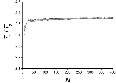
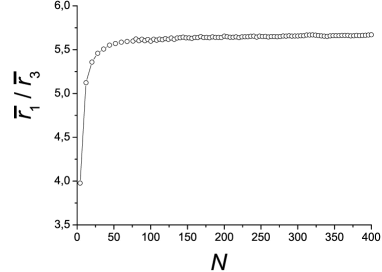
                                  a) b)

Figure 2: Ratios $\overline{r}_{1}/\overline{r}_{2}$ (a) and $\overline{r}_{1}/\overline{r}_{3}$ (b) as functions of the chain length, results of computer simulations. Analytic estimates give: $\overline{r}_{1}/\overline{r}_{2}\simeq 2.55$ and $\overline{r}_{1}/\overline{r}_{3}\simeq 5.66$ (see equations (5), (9), (10)).

3 Description of polymer shape in terms of gyration tensor and combinations of its components

Let $\vec{R}_{n}=\{x_{n}^{1}\,,\ldots,x_{n}^{d}\}$ be the position vector of the $n$th monomer of a polymer chain ($n=1,\ldots,N$). The mean square of the end-to-end distance $R_{\rm e}$ of a chain thus reads:

$$\langle R_{\rm e}^{2}\rangle=\langle|\vec{R}_{N}-\vec{R}_{1}|^{2}\rangle,$$ (12)

here and below, $\langle\ldots\rangle$ denotes the averaging over the ensemble of all possible polymer chain configurations. The basic shape properties of a specified spatial conformation of the chain can be characterized [8, 9] in terms of the gyration tensor $\bf{Q}$ with components:

$$Q_{ij}=\frac{1}{N}\sum_{n=1}^{N}(x_{n}^{i}-{x^{i}_{\rm CM}})(x_{n}^{j}-{x^{j}_{\rm CM}}),\,\,\,\,\,\,i,j=1,\ldots,d,$$ (13)

with ${x^{i}_{\rm CM}}=\sum_{n=1}^{N}x_{n}^{i}/N$ being the coordinates of the center-of-mass position vector ${\vec{R}_{\rm CM}}$ .

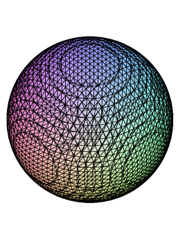
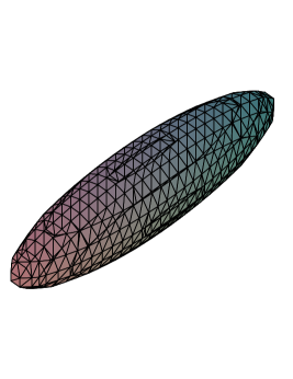
a)                                   b)                                   c)

Figure 3: Seen from far away, polymer coil may resemble the objects of different from. Here, we distinguish sphere-like (a), prolate (b), and oblate (c) conformations. Eigenvalues of corresponding gyration tensor (13) satisfy: $\lambda_{1}\simeq\lambda_{2}\simeq\lambda_{3}$ (a), $\lambda_{1}>\lambda_{2}\simeq\lambda_{3}$ (b), and $\lambda_{1}\simeq\lambda_{2}>\lambda_{3}$ (c). Correspondingly, asphericity (17) and prolateness (18) of these conformations satisfy: $A_{d}=0$, $S=0$ (a), $0<A_{d}<1$, $0<S\leqslant 2$ (b), $0<A_{d}<1$, $-1/4\leqslant S<0$ (c). See the text for more details.

The spread in the eigenvalues $\lambda_{i}$ of the gyration tensor describes the distribution of monomers inside the polymer coil and thus measures the asymmetry of the molecule; in particular, for a symmetric (spherical) configuration all the eigenvalues $\lambda_{i}$ are equal, whereas for the so-called prolate and oblate configurations in $d=3$ (see figure 3) the eigenvalues satisfy $\lambda_{1}\gg\lambda_{2}\approx\lambda_{3}$ and $\lambda_{1}\approx\lambda_{2}\gg\lambda_{3}$ correspondingly. Solc and Stockmayer [8] introduced the normalized average eigenvalues $\lambda_{i}$ of the gyration tensor as a shape measure of macromolecules. Numerical simulations in $d=3$ dimensions give $\{\langle\lambda_{1}\rangle$, $\langle\lambda_{2}\rangle$, $\langle\lambda_{3}\rangle\}$=$\{0.790,0.161,0.054\}$ [16], indicating a high anisotropy of typical polymer configurations compared with the purely isotropic case $\{1/3$, $1/3$, $1/3\}$.

While in simulations the eigenvalues of the gyration tensor ${\bf{Q}}$ can easily be calculated and averaged, different invariants have been devised for theoretical calculations. As far as ${\bf{Q}}$ has three eigenvalues in $d=3$, one may construct three independent combinations of invariants. These are the square radius of gyration $R_{\rm G}^{2}$ , the asphericity $A_{d}$ and the prolateness $S$ as elaborated in the following. The first invariant of $\bf{Q}$ is the squared radius of gyration

$$R_{\rm G}^{2}=\frac{1}{N}\sum_{n=1}^{N}(\vec{R}_{n}-{\vec{R}_{\rm CM}})^{2}=\sum_{i=1}^{d}Q_{ii}={\rm Tr}\,\bf{Q}\,,$$ (14)

which measures the distribution of monomers with respect to the center of mass. To characterize the size measure of a single flexible polymer chain, one usually considers the mean-squared end-to-end distance $\langle R_{\rm e}^{2}\rangle$ (12) and radius of gyration $\langle R_{\rm G}^{2}\rangle$ (14), both governed by the same scaling law:

$$\langle R_{\rm e}^{2}\rangle\sim\langle R_{\rm G}^{2}\rangle\sim N^{2\nu},$$ (15)

where $N$ is the mass of the macromolecule (number of monomers in a polymer chain) and $\nu$ is a universal exponent ($\nu>1/2$ $(d<4)$, $\nu=1/2$ $(d\geqslant 4)$). The ratio of these two characteristic distances, the so-called size ratio:

$$g_{d}\equiv\langle R_{\rm e}^{2}\rangle/\langle R_{\rm G}^{2}\rangle,$$ (16)

appears to be a universal, rotationally-invariant quantity ($g_{d}>6$ $(d<4)$, $g_{d}=6$ $(d\geqslant 4)$) [15].

Let ${\overline{\lambda}}\equiv{\rm Tr}\,{\bf{Q}}/d$ be the mean eigenvalue of the gyration tensor. Then one may characterize the extent of asphericity of a polymer chain configuration by the quantity ${A_{d}}$ defined as [10]:

$${A_{d}}=\frac{1}{d(d-1)}\sum_{i=1}^{d}\frac{(\lambda_{i}-{\overline{\lambda}})^{2}}{\overline{\lambda}^{2}}=\frac{d}{d-1}\frac{\rm{Tr}\,\bf{\hat{Q}}^{2}}{(\rm{Tr}\,{\bf{Q}})^{2}}\,,$$ (17)

with ${\bf{{\hat{Q}}}}\equiv{\bf{Q}}-\overline{\lambda}\,{\bf{I}}$ (here $\bf{I}$ is the unity matrix). This universal quantity equals zero for a spherical configuration, where all the eigenvalues are equal, $\lambda_{i}=\overline{\lambda}$, and takes a maximum value of one in the case of a rod-like configuration, where all the eigenvalues equal zero except one. Thus, the inequality holds: $0\leqslant A_{d}\leqslant 1$. Another rotational invariant quantity, defined in three dimensions, is the so-called prolateness $S$:

$$S=\frac{\prod_{i=1}^{3}(\lambda_{i}-{\overline{\lambda}})}{{\overline{\lambda}}^{3}}=27\frac{{\rm det}\bf{{\hat{Q}}}}{(\rm{Tr}\,{\bf{Q}})^{3}}\,.$$ (18)

If the polymer is absolutely prolate, rod-like ($\lambda_{1}\neq 0$, $\lambda_{2}=\lambda_{3}=0$), it is easy to see that $S$ equals two. For absolutely oblate, disk-like conformations ($\lambda_{1}=\lambda_{2}$ , $\lambda_{3}=0$), this quantity takes on a value of $-1/4$, while for a spherical configuration $S=0$. In general, $S$ is positive for prolate ellipsoid-like polymer conformations ($\lambda_{1}\gg\lambda_{2}\approx\lambda_{3}$) and negative for oblate ones ($\lambda_{1}\approx\lambda_{2}\gg\lambda_{3}$), whereas its magnitude measures how much oblate or prolate the polymer is. Note that since $\overline{\lambda}$ and the quantities in (14)–(18) are expressed in terms of rotational invariants, there is no need to explicitly determine the eigenvalues $\lambda_{i}$ which greatly simplifies the calculations.

The average of the quantities (14)–(18) for a given polymer chain length $N$, denoted as $\langle\ldots\rangle$, is performed over an ensemble of possible configurations of a chain. Note that some analytical and numerical approaches avoid the averaging of the ratio in (17), (18) and evaluate the ratio of averages:

$$\hat{A}_{d}=\frac{1}{d(d-1)}\sum_{i=1}^{d}\frac{\langle(\lambda_{i}-{\overline{\lambda}})^{2}\rangle}{\langle\overline{\lambda}^{2}\rangle}\,,\qquad\hat{S}=\frac{\prod_{i=1}^{3}\langle(\lambda_{i}-{\overline{\lambda}})\rangle}{\langle{\overline{\lambda}}^{3}\rangle}\,,$$ (19)

which should be distinguished from the averaged asphericity and prolateness:

$$\langle{A_{d}}\rangle=\frac{1}{d(d-1)}\left\langle\sum_{i=1}^{d}\frac{(\lambda_{i}-{\overline{\lambda}})^{2}}{\overline{\lambda}^{2}}\right\rangle,\qquad\langle{S}\rangle=\left\langle\frac{\prod_{i=1}^{3}(\lambda_{i}-{\overline{\lambda}})}{{\overline{\lambda}}^{3}}\right\rangle.$$ (20)

Contrary to $\langle{A_{d}}\rangle$ and $\langle{S}\rangle$, the quantities (19) have no direct relation to the probability distribution of the shape parameters $A_{d}$ and $S$. As pointed out by Cannon [11], this definition overestimates the effect of larger polymer configurations on the mean shape properties and suppresses the effect of compact ones. This artificially leads to overestimated values for shape parameters. The difference between $\langle{A_{d}}\rangle$ and $\hat{A}_{d}$ was found to be great (see table 1).

Table 1: Size ratio, averaged asphericity and prolateness of flexible polymer chains on regular two- and three-dimensional lattices. MC: Monte Carlo simulations, DR: direct renormalization approaches. $a$: reference [13], $b$: [12], $c$: [17], $d$: [10], $e$: [14].

$d$	Method	$g_{d}$	$\langle A_{d}\rangle$	$\hat{A}_{d}$	$\langle S\rangle$	$\hat{S}$
2	MC	$7.14\pm 0.03^{a}$	$0.501\pm 0.003^{b}$	$0.625\pm 0.008^{b}$	–	–
2	DR	$7.003^{c}$	–	$0.558^{d}$	–	$0.899^{d}$
3	MC	$6.249\pm 0.03^{e}$	$0.431\pm 0.002^{e}$	$0.546\pm 0.008^{b}$	$0.541\pm 0.004^{e}$	–
3	DR	$6.258^{c}$	$0.415^{e}$	$0.529^{d}$	–	$0.893^{d}$

Numerous experimental studies indicate that a typical flexible polymer chain in good solvent takes on the shape of an elongated, prolate ellipsoid, similar to what was shown in section 3 for a random walk. In particular, using the data of x-ray crystallography and cryo-electron microscopy, it was found that the majority of non-globular proteins are characterized by $A_{3}$ values from $0.5$ to $0.7$ and $S$ values from $0$ to $0.6$ [21, 22]. The shape parameters of polymers were analyzed analytically, based on the direct renormalization group approach [10, 14, 17], and estimated in numerical simulations [8, 12, 13, 18]. Table 1 gives typical data for the above introduced shape characteristics of long flexible polymer chains in $d=2$ and $d=3$.

Since the above shape and size characteristics of polymer macromolecules are universal, i.e. independent of the details of their chemical structure, they were (along with polymer scaling exponents) the subject of analysis by field-theoretical renormalization group approaches. In the subsequent section we will introduce this approach as used to calculate polymer shapes.

4 Field-theoretical renormalization group approach to define
polymer shape

Aronovitz and Nelson [10] developed a scheme, allowing one to compute the universal shape parameters of long flexible polymers within the frames of advanced field theory methods.

Here, we start with the Edwards continuous chain model [27], representing the polymer chain by a path ${\vec{r}}(t)$, parameterized by $0\leqslant t\leqslant T$ (see figure1 (b)). The system can be described by the effective Hamiltonian ${\cal H}$:

$${\cal H} = \frac{1}{2}\int_{0}^{T}{\rm d}\,t\left(\frac{{\rm d}\,{\vec{r}}(t)}{{\rm d}t}\right)^{2}{+}\frac{u_{0}}{4!}\int_{0}^{T}{\rm d}t\int_{0}^{T}{\rm d}t^{\prime}\delta^{d}({\vec{r}}(t)-{\vec{r}}(t^{\prime})).$$ (21)

The first term in (21) represents the chain connectivity, whereas the second term describes the short range excluded volume interaction with coupling constant $u_{0}$ .

In this scheme, the gyration tensor components (equation (13)) can be rewritten as:

$$Q_{ij}=\frac{1}{2T^{2}}\int_{0}^{T}{\rm d}\,t_{1}\int_{0}^{T}{\rm d}\,t_{2}\,\left[r^{i}(t_{1})-r^{i}(t_{2})\right]\,\left[r^{j}(t_{1})-r^{j}(t_{2})\right],\qquad i,j=1,\ldots,d.$$ (22)

The model (21) may be mapped to a field theory by a Laplace transform from the Gaussian surface $T$ to the conjugated chemical potential variable (mass) $\mu_{0}$ according to [28, 29]:

$$\hat{\cal Z}(\mu_{0})=\int{\rm d}T\exp[-\mu_{0}T]{\cal Z}(T),$$ (23)

where ${\cal Z}(T)=\int D[{\bf r}]\exp(-{\cal H})$ is the partition function of the system as function of the Gaussian surface and $\int D[{\bf r}]$ means an integration over all possible path configurations [30]. Exploiting the analogy between the polymer problem and $O(m)$ symmetric field theory in the limit $m\to 0$ (de Gennes limit) [2], it was shown [28] that the partition function of the polymer system is related to the $m=0$-component field theory with an effective Lagrangean:

$${\cal L} = \int{\rm d}^{d}x\left[\frac{1}{2}(\mu_{0}^{2}|\vec{\phi}(x)|^{2}{+}|\nabla\vec{\phi}(x)|^{2}){+}\frac{u_{0}}{4!}(\vec{\phi}^{2}(x))^{2}\right].$$ (24)

Here, $\vec{\phi}$ is an $m$-component vector field $\vec{\phi}=(\phi^{1},\ldots,\phi^{m})$ and:

$$\hat{\cal Z}(\mu_{0})=\int D[\varphi]{\rm e}^{-{\cal L}}.$$ (25)

One of the ways of extracting the scaling behavior of the model (24), is to apply the field-theoretical renormalization group (RG) method [5] in the massive scheme, with the Green’s functions renormalized at non-zero mass and zero external momenta. The Green’s function $G_{0}^{(N,L)}$ can be defined as an average of $N$ field components and $L$ $\varphi^{2}$-insertions performed with the corresponding effective Lagrangean ${\cal L}$:

$$\delta(\sum k_{i}{+}\sum p_{j})G_{0}^{(N,L)}(\{k\};\{p\};\mu^{2}_{0}\,;u_{0})=$$ (26)

$$\mbox{}\int^{\Lambda_{0}}\re^{\ri(k_{i}R_{i}{+}p_{j}r_{j})}\langle\phi^{2}(r_{1})\dots\phi^{2}(r_{L})\phi(R_{1})\dots\phi(R_{N})\rangle^{{\cal L}_{\rm eff}}{\rm d}^{d}R_{1}\dots\rm d^{d}R_{N}{\rm d}^{d}r_{1}\dots\rm d^{d}r_{L}\,,$$

here $\{k\}=(k_{1}\,,\ldots,k_{L})$, $\{p\}=(p_{1}\,,\ldots,p_{N})$ are the sets of external momenta and $\Lambda_{0}$ is a cut-off [31]. The renormalized Green’s functions $G_{\rm R}^{(N,L)}$ are expressed in terms of the bare vertex functions as follows:

$$G_{0}^{(N,L)}(\{k\};\{p\};\hat{\mu}_{0}^{2};u_{0})=Z_{\phi}^{N/2}Z_{\phi^{2}}^{-L}G_{\rm R}^{(N,L)}(\{k\};\{p\};\mu^{2};u),$$ (27)

where $Z_{\phi}$ , $Z_{\phi^{2}}$ are the renormalizing factors, $\mu$, $u$ are the renormalized mass and couplings.

The change of coupling constant $u_{0}$ under renormalization defines a flow in parametric space, governed by the corresponding $\beta$-function:

$$\beta_{u}(u)=\frac{\partial u}{\partial\ln l}\Big{|}_{0}\,,$$ (28)

where $l$ is the rescaling factor and $\big{|}_{0}$ stands for evaluation at fixed bare parameters. The fixed points (FP) of the RG transformation are given by the zeroes of the $\beta$-function. The stable FP $u^{*}$, corresponding to the critical point of the system, is defined as the fixed point where $\frac{\partial\beta_{u}(u)}{\partial u}|_{u=u^{*}}$ has a positive real part. The flow of renormalizing factors $Z_{\phi}$ , $Z_{\phi^{2}}$ defines the RG functions $\gamma_{\phi}(u)$, ${\bar{\gamma}}_{\phi^{2}}(u)$. These functions, evaluated at the stable accessible FP, allow us to estimate the critical exponents.

Exploiting the perturbation theory expansion in parameter $\varepsilon=4-d$ (deviation of space dimension from the upper critical one), one receives within the above described scheme up to the first order in $\varepsilon$ the well-known results for the fixed points:

$$u^{*}_{\rm RW}=0\,,\hskip 7.11317pt \varepsilon\leqslant 0,$$ stable for (29)

$$u^{*}_{\rm SAW}=\frac{3\varepsilon}{4}\,, \varepsilon>0.$$ stable for (30)

Here, $u_{\rm RW}$ describes the case of simple random walks (idealized polymer chain without any intrachain interactions), and $u_{\rm SAW}$ is the fixed point, governing the scaling of self-avoiding random walks.

Evaluating the RG functions $\gamma_{\phi}(u)$ and ${\bar{\gamma}}_{\phi^{2}}(u)$ at the above fixed points, one gets the familiar first-order results (see e.g. [5]) for the critical exponents $\nu$ and $\gamma$, that govern the scaling of the polymer mean size (15) and the number of configurations, correspondingly:

$$\nu_{\rm RW\phantom{I}}=\frac{1}{2}\,,\qquad\quad\,\,\,\gamma_{\rm RW\phantom{I}}=1\,,$$ (31)

$$\nu_{\rm SAW}=\frac{1}{2}{+}\frac{\varepsilon}{16}\,,\quad\,\,\,\gamma_{\rm SAW}=1{+}\frac{\varepsilon}{8}\,.$$ (32)

Following reference [10], the averaged moments of gyration tensor $\bf{Q}$ (22), which are needed to determine the polymer shape characteristics (14), (17), (18), can be expressed in terms of renormalized connected Green’s functions (27), in particular:

$$\langle Q_{ij}\rangle=-\frac{1}{2}\left(\frac{T}{2\bar{X}}\right)^{2\nu}\frac{\Gamma(\gamma)}{\Gamma(\gamma{+}2\nu{+}2)}\frac{G_{ij}}{G_{\rm R}^{(2)}(0,0,u^{*})}\,,$$ (33)

$$\langle Q_{ij}Q_{kl}\rangle=-\frac{1}{4}\left(\frac{T}{2\bar{X}}\right)^{4\nu}\frac{\Gamma(\gamma)}{\Gamma(\gamma{+}4\nu{+}4)}\frac{G_{ij|kl}}{G_{\rm R}^{(2)}(0,0,u^{*})}\,.$$ (34)

Here, the following notations are used:

$$G_{ij}\equiv\frac{\partial}{\partial q^{i}}\frac{\partial}{\partial q^{j}}\Big{|}_{q=0}G_{\rm R}^{(2,2)}(0,0;{q},-{q};u^{*}),$$ (35)

$$G_{ij|kl}={\frac{\partial}{\partial q^{i}_{1}}\frac{\partial}{\partial q^{j}_{1}}\frac{\partial}{\partial q^{k}_{2}}\frac{\partial}{\partial q^{l}_{2}}\Big{|}_{{q}=0}G_{\rm R}^{(2,4)}(0,0;{q}_{1}\,,-{q}_{1}\,,{q}_{2}\,,-{q}_{2}\,;u^{*})},$$ (36)

$\bar{X}$ is non-universal quantity, $\nu$ and $\gamma$ are the critical exponents, ${\partial}/{\partial q_{1}^{i}}$ means differentiation by the $i$-component of vector $q_{1}$ , $G_{\rm R}^{(2,2)}$ and $G_{\rm R}^{(2,4)}$ are the renormalized connected Green’s function with 2 external legs and 2 insertions $\varphi^{2}(q)$, $\varphi^{2}(-q)$ and 4 insertions $\varphi^{2}(q_{1})$, $\varphi^{2}(-q_{1})$, $\varphi^{2}(q_{2})$, $\varphi^{2}(-q_{2})$ respectively, calculated at the fixed point for zero external momenta.

The isotropy of the original theory implies, in particular, that $\langle{\rm Tr{\bf{Q}}}\rangle=d\langle Q_{ii}\rangle$, so that:

$$\langle R_{\rm G}^{2}\rangle=d\langle Q_{ii}\rangle.$$ (37)

The mean-squared end-to-end distance $\langle R_{\rm e}^{2}\rangle$ can be expressed as:

$$\langle R_{\rm e}^{2}\rangle=-\left(\frac{T}{2\bar{X}}\right)^{2\nu}\frac{\Gamma(\gamma)}{\Gamma(\gamma{+}2\nu)}\frac{\left(\nabla_{{k}}^{2}G_{\rm R}^{(2)}({k},-{k},u^{*})\right)\Big{|}_{{k}=0}}{G_{\rm R}^{(2)}(0,0,u^{*})}\,.$$ (38)

where $\nabla_{{k}}^{2}$ means differentiation over components of external momentum ${k}$.

One can easily convince oneself, that not-universal quantities cancel when the ratio (16) is considered:

$$g\equiv\frac{\langle R_{\rm e}^{2}\rangle}{\langle R_{\rm G}^{2}\rangle}=\frac{\Gamma(\gamma{+}2\nu{+}2)}{\Gamma(\gamma{+}2\nu)}\frac{\left(\nabla_{{k}}^{2}G_{\rm R}^{(2)}(k,-k,u^{*})\right)\Big{|}_{{k}=0}}{\left(\nabla_{{q}}^{2}G_{\rm R}^{(2,2)}(0,0;{q},-{q};u^{*})\right)\Big{|}_{{q}=0}}\,.$$ (39)

In derivation of (39) we made use of an obvious relation $\sum_{i=1}^{d}G_{ii}=\nabla^{2}G_{\rm R}^{(2,2)}$.

Figure 4: Contributions to the Green’s function $G^{(2,2)}$ up to one-loop level. Solid lines denote propagators $\mu^{2}{+}k^{2}$, wavy lines illustrate the insertions of the type $\varphi^{2}$, loops imply integration over internal momenta.

Figure 5: Contributions to the Green’s function $G^{(2,4)}$ up to one-loop level. Solid lines denote propagators $\mu^{2}{+}k^{2}$, wavy lines illustrate the insertions of the type $\varphi^{2}$, loops imply integration over internal momenta.

Computing the asphericity we follow equation (19) considering $\hat{A}_{d}$ as the ratio of averages:

$$\hat{A}_{d}=\frac{d}{d-1}\frac{\langle{\rm{Tr}}\,{\bf{{\hat{Q}}}}^{2}\rangle}{\langle(\rm{Tr}\,{\bf{Q}})^{2}\rangle}\,.$$ (40)

This definition allows one to directly apply the renormalization group scheme described above, and express the $\hat{A}_{d}$ in terms of the averaged moments of the gyration tensor (33), (34):

$$\hat{A}_{d}=\frac{\langle Q_{ii}^{2}\rangle{+}d\langle Q_{ij}^{2}\rangle-\langle Q_{ii}Q_{jj}\rangle}{\langle Q_{ii}^{2}\rangle{+}d(d-1)\langle Q_{ii}Q_{jj}\rangle}\,,\qquad i\neq j.$$ (41)

One can again easily convince oneself that all the non-universal quantities in equations (33), (34) cancel when calculating (41). Note that within the RG approach we will focuss only on two universal shape characteristics, namely the size ratio (39) and asphericity (41), as far as the calculation of prolateness $S$ is particularly cumbersome.

To estimate (39), one needs to calculate the Green’s functions $G^{(2,2)}$, presented diagrammatically in figure 4. Applying the renormalization procedure, as described above, one finds to the first order of the renormalized coupling $u$ (i.e., in the so-called one-loop approximation):

$$G_{\rm R}^{(2,2)}(0,0;{q},-{q};u)=\frac{2}{q^{2}{+}1}-\frac{4}{3}\frac{1}{q^{2}{+}1}uI_{1}(0,q)-\frac{2}{3}uI_{2}(0,0,q){+}\frac{4}{3}\frac{1}{q^{2}{+}1}uI_{1}(0,0),$$ (42)

the one-loop integrals $I_{i}$ are listed in appendix A. Performing an $\varepsilon=4-d$-expansion of loop integrals (see appendix A for details) and differentiating over components of vector ${q}$, we found:

$$\left(\nabla_{{q}}^{2}G_{\rm R}^{(2,2)}(0,0;{q},-{q};u)\right)\Big{|}_{{q}=0}=-4-\frac{19}{18}u,$$ (43)

$$\left(\nabla_{{k}}^{2}G_{\rm R}^{(2)}(k,-k)\right)\Big{|}_{{k}=0}=-2.$$ (44)

Substituting the values of fixed points (29) and (30) into the ratio of these functions, one receives the corresponding value of the $g$-ratio:

$$g_{\rm RW\phantom{I}}=6\,,$$ (45)

$$g_{\rm SAW}=6{+}\frac{\varepsilon}{16}\,.$$ (46)

Equation (46) presents a first order correction to the $g$-ratio caused by excluded volume interactions.

To compute the averaged asphericity ratio using (41), one needs the Green function $G^{(2,4)}$ with four insertions $\varphi^{2}({q}_{1})/2$, $\varphi^{2}(-{q}_{1})/2$, $\varphi^{2}({q}_{2})/2$, $\varphi^{2}(-{q}_{2})/2$, which is schematically presented in figure 5. Applying the renormalization scheme described above, one receives an analytic expression for the renormalized function $G_{\rm R}^{(2,4)}$, given in the appendix B, equation (Appendix B). Taking derivatives over components of inserted vectors ${q}_{1}$ , ${q}_{2}$ and performing $\varepsilon$-expansions of the resulting expressions (see appendix A for details) we arrive at the following expansions for the functions (35), (36):

$$G_{xx\phantom{|yy}}=576{+}\frac{4028u}{15}\,,$$

$$G_{xx|yy}=320{+}\frac{436u}{3}\,,$$

$$G_{xy|xy}=128{+}\frac{308u}{5}\,.$$ (47)

Evaluating these relations at the fixed points (29), (30) and substituting into (33), (34), (41) one receives:

$$\hat{A}_{d}^{\rm RW\phantom{I}}=\frac{1}{2}\,,$$ (48)

$$\hat{A}_{d}^{\rm SAW}=\frac{1}{2}{+}\frac{15}{512}\varepsilon\,.$$ (49)

We note, that result (48) means that even within the idealized model of simple random walks, the shape of a polymer chain is highly anisotropic (cf. Kuhn’s picture, described in section 2). Taking into account the excluded volume effect makes the polymer chain more extended and aspherical: indeed, in three dimensions ($\varepsilon=1$) the above obtained quantity reads: $\hat{A}_{d}^{\rm SAW}\simeq 0.53$.

5 Polymer in porous environment: Model with long-range correlated disorder

In real physical processes, one is often interested how structural obstacles (impurities) in the environment alter the behavior of a system. The density fluctuations of obstacles lead to a large spatial inhomogeneity and create pore spaces, which are often of fractal structure [32]. In polymer physics, it is of great importance to understand the behavior of macromolecules in the presence of structural disorder, e.g., in colloidal solutions [33] or near the microporous membranes [34]. In particular, a related problem concerns the protein folding dynamics in the cellular environment, which can be considered as a highly disordered environment due to the presence of a large amount of biochemical species, occupying up to $40\%$ of the total volume [35]. Structural obstacles strongly affect the protein folding [36]. Recently, it was realized experimentally [37] that macromolecular crowding has a dramatic effect on the shape properties of proteins.

In the language of lattice models, a disordered environment with structural obstacles can be considered as a lattice, where some amount of randomly chosen sites contain defects which are to be avoided by the polymer chain. Of particular interest is the case when the concentration of lattice sites allowed for the SAWs equals the critical concentration and the lattice is at the percolation threshold. In this regime, SAWs belong to a new universality class, the scaling law (15) holds with exponent $\nu_{\rm p_{c}}>\nu_{{\rm SAW}}$ [38]. The universal shape characteristics of flexible polymers in disordered environments modeled by a percolating lattice were studied recently in [39]. Another interesting situation arises when the structural obstacles of environment display correlations on a mesoscopic scale [40]. One can describe such a medium by a model of long-range-correlated (extended) quenched defects. This model was proposed in reference [41] in the context of magnetic phase transitions. It considers defects, characterized by a pair correlation function $h(r)$, that decays with a distance $r$ according to a power law:

$$h(r)\sim r^{-a}$$ (50)

at large $r$. This type of disorder has a direct interpretation for integer values of $a$; namely, the case $a=d$ corresponds to point-like defects, while $a=d-1$ $(a=d-2)$ describes straight lines (planes) of impurities of random orientation. Non-integer values of $a$ are interpreted in terms of impurities organized in fractal structures [42]. The effect of this type of disorder on the magnetic phase transitions has been a subject to numerous studies [43].

The impact of long-range-correlated disorder on the scaling of single polymer chains was analyzed in our previous works [44] by means of field-theoretical renormalization group approach. In particular, it was shown that the correlated obstacles in environment lead to a new universality class with values of the polymer scaling exponents that depend on the strength of correlation expressed by parameters $a$. The question about how the characteristics of shape of a flexible chain are effected by the presence of such a porous medium was briefly discussed by us in reference [45]. The details of these calculations will be presented here.

We introduce disorder into the model (24), by redefining $\mu_{0}^{2}\to\mu_{0}^{2}{+}\delta\mu_{0}(x)$, where the local fluctuations $\delta\mu_{0}(x)$ obey:

$$\langle\langle\delta\mu_{0}(x)\rangle\rangle =0,$$

$$\langle\langle\delta\mu_{0}(x)\delta\hat{\mu}_{0}(y)\rangle\rangle =h(|x-y|).$$ (51)

Here, $\langle\langle\ldots\rangle\rangle$ denotes the average over spatially homogeneous and isotropic quenched disorder. The form of the pair correlation function $h(r)$ is chosen to decay with distance according to (50).

In order to average the free energy over different configurations of the quenched disorder we apply the replica method to construct an effective Lagrangean [44]:

$${\cal L}_{\rm dis} = \frac{1}{2}\sum_{\alpha=1}^{n}\int{\rm d}^{d}x\left[\left(\mu_{0}^{2}|\vec{\phi}_{\alpha}(x)|^{2}{+}|\nabla\vec{\phi}_{\alpha}(x)|^{2}\right){+}\frac{u_{0}}{4!}\left(\vec{\phi}^{2}_{\alpha}(x)\right)^{2}\right]$$ (52)

$${+} \sum_{\alpha,\beta=1}^{n}\int{\rm d}^{d}x{\rm d}^{d}yh(|x-y|)\vec{\phi}_{\alpha}^{2}(x)\vec{\phi}_{\beta}^{2}(y).$$

Here, the term describing replicas coupling contains the correlation function $h(r)$ (50), Greek indices denote replicas and both the replica ($n\to 0$) and polymer ($m\to 0$) limits are implied. For small $k$, the Fourier-transform $\tilde{h}(k)$ of (50) reads:

$$\tilde{h}(k)\sim v_{0}{+}w_{0}|k|^{a-d}.$$ (53)

Taking this into account, rewriting equation (52) in momentum space variables, and recalling the special symmetry properties of (52) that appear for $m$, $n\to 0$ [44], a theory with two bare couplings $u_{0}$ , $w_{0}$ results. Note that for $a\geqslant d$ the $w_{0}$-term is irrelevant in the RG sense and one restores the pure case (absence of structural disorder). As it will be shown below, this term modifies the critical behaviour at $a<d$. We will refer to this type of disorder as long-range-correlated and denote by LR hereafter.

To extract the scaling behavior of the model (52), one applies the field-theoretical renormalization group method following the scheme described in a previous section, with modifications caused by the presence of the second coupling constant $w_{0}$ . In particular, the change of couplings $u_{0}$ , $w_{0}$ under renormalization defines a flow in parametric space, governed by corresponding $\beta$-functions (c.f. equation (28)):

$$\beta_{u}(u,w)=\frac{\partial u}{\partial\ln l}\Big{|}_{0}\,,\qquad\beta_{w}(u,w)=\frac{\partial w}{\partial\ln l}\Big{|}_{0}\,.$$ (54)

The fixed points (FPs) of the RG transformation are given by common zeroes of the $\beta$-functions. The stable FP ($u^{*}$, $w^{*}$) that corresponds to the critical point of the system, is defined as the fixed point where the stability matrix $B_{ij}={\partial\beta_{\lambda_{i}}}/{\partial\lambda_{j}}$ , $i,j=1,2$ possesses eigenvalues with positive real parts (here, $\lambda_{1}=u$, $\lambda_{2}=w$).

In our previous work [44] we have found the FP coordinates for polymers in LR disorder, which up to the first order of $\varepsilon=4-d$, $\delta=4-a$-expansion read:

$$u^{*}_{\rm RW\phantom{I}}=0, w^{*}_{\rm RW\phantom{I}}=0 \text{stable for}\quad\delta<0,\,\delta<0,$$ (55)

$$u^{*}_{\rm SAW}=\frac{3\varepsilon}{4}\,, w^{*}_{\rm SAW}=0 \text{stable for}\quad\delta<\varepsilon/2,$$ (56)

$$u^{*}_{\rm LR\phantom{B}}=\frac{3\delta^{2}}{2(\varepsilon-\delta)}\,, w^{*}_{\rm LR\phantom{B}}=\frac{3\delta(\varepsilon-2\delta)}{2(\varepsilon-\delta)} \text{stable for}\quad\varepsilon/2<\delta<\varepsilon.$$ (57)

The RW and SAW fixed points restore the corresponding cases of a polymer in pure solvent (cf. (29), (30)), whereas the LR fixed point reflects the effect of correlated obstacles, which appears to be non-trivial in certain regions of the $d$, $a$ plane and to govern new scaling behaviour in this region. For critical exponents $\nu_{\rm LR}$, $\gamma_{\rm LR}$ governing the scaling of polymer chains in the region of $a$, $d$, where the effect of LR disorder is nontrivial, one obtains [44]:

$$\nu_{\rm LR}=1/2{+}\delta/8,\qquad\gamma_{\rm LR}=1{+}\delta/4.$$ (58)

As it was explained in the previous section, to estimate the universal size ratio (39) for the case of polymers in long-range-correlated disorder, we calculate the Green function $G^{(2,2)}(u,w)$, presented diagrammatically in figure 4. Now, every interactive diagram appears twice, once with each of the two couplings $u$ and $w$, respectively. For the renormalized function we obtain up to the one-loop approximation:

$$G_{\rm R}^{(2,2)}(0,0;{q},-{q};u,w)=\frac{2}{q^{2}{+}1}-\frac{4}{3}\frac{1}{q^{2}{+}1}\left[uI_{1}(0,q)-wJ_{1}(0,q)\right]$$

$$-\frac{2}{3}\left[uI_{2}(0,0,q)-wJ_{2}(0,0,q)\right]{+}\frac{4}{3}\frac{1}{q^{2}{+}1}\left[uI_{1}(0,0)-wJ_{1}(0,0)\right].$$ (59)

The one-loop integrals $I_{i}$ are given in appendix A. Note that $J_{i}$ differs from corresponding $I_{i}$ only by an additional factor $|p|^{a-d}$ in the numerator. Differentiating over components of vector ${q}$, evaluating at ${q}=0$ and performing double $\varepsilon,\delta$-expansions of the resulting expression, we have:

$$\left(\nabla_{{q}}^{2}G_{\rm R}^{(2,2)}(0,0;{q},-{q};u,w)\right)\Big{|}_{{q}=0}=-4-\frac{19}{18}u-\frac{19}{18}w,$$ (60)

$$\left(\nabla_{{k}}^{2}G_{\rm R}^{(2)}(k,-k)\right)\Big{|}_{{k}=0}=-2.$$ (61)

Recalling the value of the LR fixed point (57), and inserting this into the ratio (39) of these functions, one arrives at an expansion for the size ratio of a SAW in the presence of long-range correlated disorder:

$$g_{\rm LR}=6{+}\frac{\delta}{8}\,.$$ (62)

This should be compared with the corresponding value in the pure case (46). Let us qualitatively estimate the change in the size ratio $g$, caused by the presence of structural obstacles in three dimensions. Substituting directly $\varepsilon=1$ into (46), we have for the polymer chain in a pure solvent: $g^{{\rm pure}}\simeq 6.06.$ Let us recall that the effect of long-range-correlated disorder is relevant to $a\leqslant d$ ($\delta\geqslant\varepsilon$) (see e.g. explanation after equation (52)). Estimates of $g_{{\rm LR}}$ can be evaluated by direct substitution of the continuously variable parameter $\delta$ into equation (62). One concludes that increasing the parameter $\delta$ (which corresponds to an increase of disorder strength) leads to a corresponding increase of the $g$-ratio.

To compute the averaged asphericity in correspondence with (41), we need the Green function $G^{(2,4)}(u,w)$ with four insertions $\varphi^{2}({q}_{1})/2$, $\varphi^{2}(-{q}_{1})/2$, $\varphi^{2}({q}_{2})/2$, $\varphi^{2}(-{q}_{2})/2$, shown diagrammatically in figure 5. The corresponding analytic expression for the renormalized function is given in appendix B, equation (Appendix B). Taking derivatives of this expression with respect to the components of the inserted vectors ${q}_{1}$, ${q}_{2}$ we find:

$$G_{xx\phantom{|yy}}=576{+}\frac{4028}{15}(u-w),$$

$$G_{xx|yy}=320{+}\frac{436}{3}(u-w),$$

$$G_{xy|xy}=128{+}\frac{308}{5}(u-w).$$ (63)

At the LR fixed point (57), from (41) we finally have:

$$\hat{A}_{d}^{\rm LR}=\frac{1}{2}{+}\frac{1}{48}\,\varepsilon{+}\frac{13}{768}\,\delta.$$ (64)

Again, let us qualitatively estimate the change in $\hat{A}_{d}$ caused by the presence of structural obstacles in three dimensions. Substituting directly $\varepsilon=1$ into (49), we have for the pure case: $\hat{A}_{d}^{{\rm pure}}\simeq 0.53$. Estimates of $\hat{A}_{d}^{{\rm LR}}$ can be obtained by direct substitution of the continuously changing parameter $\delta$ into equation (64). An increasing strength of disorder correlations results in an increase of the asphericity ratio of polymers in disorder. This phenomenon is intuitively understandable if one recalls the impact of the long-range-correlated disorder on the mean end-to-end distance exponent $\nu$. Indeed, it has been shown in [44] that such disorder leads to an increase of $\nu$, and subsequently, to the swelling of a polymer chain. Extended obstacles do not favour return trajectories and as a result the polymer chain becomes more elongated. In turn, such elongation leads to an increase of the asphericity ratio as predicted by equation (64).

6 Conclusions

The universal characteristics of the average shape of polymer coil configurations in a porous (crowded) environment with structural obstacles have been analyzed considering the special case when the defects are correlated at large distances $r$ according to a power law: $h(r)\sim r^{-a}$. Applying the field-theoretical RG approach, we estimate the size ratio $g=\langle R_{\rm e}^{2}\rangle/\langle R_{\rm G}^{2}\rangle$ and averaged asphericity ratio $\hat{A_{d}}$ up to the first order of a double $\varepsilon=4-d$, $\delta=4-a$ expansion. We have revealed that the presence of long-range-correlated disorder leads to an increase of both $g$ and $\hat{A_{d}}$ as compared to their values for a polymer chain in a pure solution. Moreover, the value of the asphericity ratio $\hat{A_{d}}$ was found to be closer to the maximal value of one in presence of correlated obstacles. Thus, we conclude that the presence of structural obstacles in an environment enforces the polymer coil configurations to be less spherical. We believe that the obtained first order results indicate the appropriate qualitative changes in polymer shape caused by long-range-correlated environment. However, to get more accurate quantitative results, higher orders of perturbation theory may be needed. This is subject of further investigations.

Appendix A

Here, we present the expressions for the loop integrals, as they appear in the Green functions $G^{(2,2)}$ and $G^{(2,4)}$. We make the couplings dimensionless by redefining $u=u\,\mu^{d-4}$ and $w=w\,\mu^{a-4}$; therefore, the loop integrals do not explicitly contain the mass [31]:

$$I_{1}(k_{1},k_{2})=\int\frac{{\rm d}{\vec{p}}}{\left[(p{+}k_{1})^{2}{+}1\right]\left[(p{+}k_{2})^{2}{+}1\right]}\,,$$

$$I_{2}(k_{1},k_{2}\,,k_{3})=\int\frac{{\rm d}{\vec{p}}}{[(p{+}k_{1})^{2}{+}1][(p{+}k_{2})^{2}{+}1][(p{+}k_{3})^{2}{+}1]}\,,$$

$$I_{3}(k_{1},k_{2}\,,k_{3}\,,k_{4})=\int\frac{{\rm d}{\vec{p}}}{[(p{+}k_{1})^{2}{+}1][(p{+}k_{2})^{2}{+}1][(p{+}k_{3})^{2}{+}1][(p{+}k_{4})^{2}{+}1]}\,,$$

$$I_{4}(k_{1},k_{2}\,,k_{3}\,,k_{4}\,,k_{5})=\int\frac{{\rm d}{\vec{p}}}{[(p{+}k_{1})^{2}{+}1][(p{+}k_{2})^{2}{+}1][(p{+}k_{3})^{2}{+}1][(p{+}k_{4})^{2}{+}1][(p{+}k_{5})^{2}{+}1]}\,.$$

The loop integrals $J_{i}$ (equations (59) and (Appendix B)) differ from corresponding $I_{i}$ only by an additional factor $|p|^{a-d}$ in the numerators. The correspondence of the integrals to the diagrams in figure 5 is:

$$(e),(f): \text{integrals}\quad I_{1}(0,q_{1}),\,I_{1}(0,q_{2}),\,J_{1}(0,q_{1}),\,J_{1}(0,q_{2}),$$

$$(g): I_{2}(0,q_{1}\,,q_{2}),\,I_{2}(0,0,q_{1}),\,I_{2}(0,0,q_{2}),\,J_{2}(0,q_{1}\,,q_{2}),\,J_{2}(0,0,q_{1}),\,J_{2}(0,0,q_{2}),$$

$$J_{2}(0,q_{1}\,,q_{2}),\,J_{2}(0,0,q_{1}),\,J_{2}(0,0,q_{2}),$$

$$(h): I_{2}(0,0,q_{1}),\,I_{2}(0,0,q_{2}),\,I_{2}(0,q_{1}\,,q_{1}{+}q_{2}),\,I_{2}(0,q_{2}\,,q_{1}{+}q_{2}),\,J_{2}(0,0,q_{1}),$$

$$J_{2}(0,0,q_{2}),\,J_{2}(0,q_{1}\,,q_{1}{+}q_{2}),\,J_{2}(0,q_{2}\,,q_{1}{+}q_{2}),$$

$$(i): I_{3}(0,0,q_{1}\,,q_{2}),\,I_{3}(0,q_{1}\,,q_{2}\,,q_{1}{+}q_{2}),\,I_{3}(0,q_{1}\,,q_{1}\,,q_{1}{+}q_{2}),\,I_{3}(0,q_{2}\,,q_{2}\,,q_{1}{+}q_{2}),$$

$$J_{3}(0,0,q_{1}\,,q_{2}),\,J_{3}(0,q_{1}\,,q_{2}\,,q_{1}{+}q_{2}),\,J_{3}(0,q_{1}\,,q_{1}\,,q_{1}{+}q_{2}),\,J_{3}(0,q_{2}\,,q_{2}\,,q_{1}{+}q_{2}),$$

$$(j): I_{4}(0,0,0,q_{1}\,,q_{2}),\,I_{4}(0,0,q_{1}\,,q_{2}\,,q_{1}{+}q_{2}),\,I_{4}(0,0,q_{1}\,,q_{1}\,,q_{1}{+}q_{2}),\,I_{4}(0,0,q_{2}\,,q_{2}\,,q_{1}{+}q_{2}),$$

$$J_{4}(0,0,0,q_{1}\,,q_{2}),\,J_{4}(0,0,q_{1}\,,q_{2}\,,q_{1}{+}q_{2}),\,J_{4}(0,0,q_{1}\,,q_{1}\,,q_{1}{+}q_{2}),\,J_{4}(0,0,q_{2}\,,q_{2}\,,q_{1}{+}q_{2}).$$

In our calculations, we use the following formula to fold many denominators into one (see e.g. book of D. Amit in reference [5]):

$$\frac{1}{a_{1}^{\alpha_{1}}\ldots a_{n}^{\alpha_{n}}}=\frac{\Gamma(\alpha_{1}{{+}}\ldots{{+}}\alpha_{n})}{\Gamma(\alpha_{1})\ldots\Gamma(\alpha_{n})}\times$$ (A65)

$$\mbox{}\times\int\limits_{0}^{1}{\rm d}x_{1}\!\!\ldots\!\!\int\limits_{0}^{1}{\rm d}x_{n-1}\frac{x_{1}^{\alpha_{n}-1}\ldots x_{n-1}^{\alpha_{n-1}-1}(1{-}x_{1}{-}\ldots{-}x_{n-1})^{\alpha_{n}-1}}{[x_{1}a_{1}{{+}}\ldots{{+}}x_{n-1}a_{n-1}{{+}}(1{-}x_{1}{-}\ldots{-}x_{n-1})a_{n}]^{\alpha_{1}{+}\ldots{+}\alpha_{n}}}\,,$$

where the Feynmann variables $x_{i}$ extend over the domain $x_{1}+\ldots+x_{n-1}\leqslant 1$.

To compute the $d$-dimensional integrals we apply :

$$\int\frac{{\rm d}{p}}{(p^{2}{+}2\vec{k}\vec{p}{+}m^{2})^{\alpha}}=\frac{1}{2}\frac{\Gamma(d/2)\Gamma(\alpha-d/2)}{\Gamma(\alpha)}(m^{2}-k^{2})^{d/2-\alpha},$$ (A66)

here ${\rm d}p={\rm d}^{d}p\,\Omega_{d}/(2\pi)^{d}$, where the geometrical angular factor $\Omega_{d}=1/(2^{d-1}\pi^{d/2}\Gamma(d/2))$ is separated out and absorbed by redefining the coupling constant.

As an example we present the calculation of the integral:

$$I_{2}(0,q_{1}\,,q_{2})=\int\frac{{\rm d}{\vec{p}}}{(p^{2}{+}1)[(p{+}q_{1})^{2}{+}1][(p{+}q_{2})^{2}{+}1]}\,.$$ (A67)

First, we make use of formula (A65) to rewrite:

$$\frac{1}{(p^{2}{+}1)[(p{+}q_{1})^{2}{+}1][(p{+}q_{2})^{2}{+}1]}=\frac{\Gamma(3)\int_{0}^{1}{\rm d}x_{1}\int_{0}^{1}{\rm d}x_{2}}{[p^{2}{+}2\vec{p}(\vec{q}_{1}x_{1}{+}\vec{q}_{2}x_{2}){+}1{+}x_{1}q_{1}^{2}{+}x_{2}q_{2}^{2}]^{3}}\,.$$

Now one can perform the integration over $p$, passing to the $d$-dimensional polar coordinates and making use of the formula (A66):

$${\int\frac{{\rm d}{p}}{[p^{2}{+}2\vec{p}(\vec{q}_{1}x_{1}{+}\vec{q}_{2}x_{2}){+}1{+}x_{1}q_{1}^{2}{+}x_{2}q_{2}^{2}]^{3}}=}$$

$$\frac{\Gamma(d/2)\Gamma(3-d/2)}{2\Gamma(3)}[1{+}x_{1}q_{1}^{2}(1-x_{1}){+}x_{2}q_{2}^{2}(1-x_{2})-2x_{1}x_{2}q_{1}q_{2}]^{d/2-3}.$$ (A68)

As a result, we are left with:

$$I_{2}(0,q_{1}\,,q_{2})=\frac{1}{2}{\Gamma\left(\frac{d}{2}\right)}{\Gamma\left(3-\frac{d}{2}\right)}\times$$ (A69)

$$\mbox{}\times\int\limits_{0}^{1}{\rm d}x_{1}\int\limits_{0}^{1}{\rm d}x_{2}[1{+}x_{1}q_{1}^{2}(1-x_{1}){+}x_{2}q_{2}^{2}(1-x_{2})-2x_{1}x_{2}q_{1}q_{2}]^{d/2-3}.$$

To find the contributions of this integral to $G_{xx|xx}$ and $G_{xx|yy}$ (according to (36)), we first differentiate the integrand in (A69) over the components of vectors $\vec{q}_{1}$ , $\vec{q}_{2}$:

$$I_{xx|xx} \equiv\frac{\rd}{\rd q_{1}^{x}}\frac{\rd}{\rd q_{1}^{x}}\frac{\rd}{\rd q_{2}^{x}}\frac{\rd}{\rd q_{2}^{x}}\left[1{+}x_{1}q_{1}^{2}(1-x_{1}){+}x_{2}q_{2}^{2}(1-x_{2})-2x_{1}x_{2}q_{1}q_{2}\right]^{d/2-3}\Big{|}_{\vec{q}_{1}=\vec{q}_{2}=0}$$

$$=4\left(\frac{d}{2}-3\right)^{2}\left[2x_{1}^{2}x_{2}^{2}{+}x_{2}x_{1}(1-x_{2})(1-x_{1})\right]-4\left(\frac{d}{2}-3\right)\left[x_{1}x_{2}(1-x_{1})(1-x_{2}){+}4x_{1}^{2}x_{2}^{2}\right],$$

$$I_{xx|yy} \equiv\frac{\rd}{\rd q_{1}^{x}}\frac{\rd}{\rd q_{1}^{x}}\frac{\rd}{\rd q_{2}^{y}}\frac{\rd}{\rd q_{2}^{y}}\left[1{+}x_{1}q_{1}^{2}(1-x_{1}){+}x_{2}q_{2}^{2}(1-x_{2})-2x_{1}x_{2}q_{1}q_{2}\right]^{d/2-3}|_{\vec{q}_{1}=\vec{q}_{2}=0}$$

$$=\left(\frac{d}{2}-3\right)^{2}x_{2}x_{1}(1-x_{2})(1-x_{1})-4\left(\frac{d}{2}-3\right)x_{2}x_{1}(1-x_{1})(1-x_{2}).$$

Finally, the contributions of $I_{2}(0,q_{1}\,,q_{2})$ to $G_{xx|xx}$ and $G_{xx|yy}$ are found by performing integration of $I_{xx|xx}$ and $I_{xx|yy}$ over $x_{1}$ , $x_{2}$ in (A69). Results can further be evaluated either fixing the value of space dimension $d$ or performing an expansion in parameter $\varepsilon=4-d$. Working within the last approach, we obtain up to the first order of the $\varepsilon$-expansion:

$$\frac{1}{2}{\Gamma\left(\frac{d}{2}\right)}{\Gamma\left(3-\frac{d}{2}\right)}\int\limits_{0}^{1}{\rm d}x_{1}\int\limits_{0}^{1}{\rm d}x_{2}\,I_{xx|xx}\simeq\frac{1}{9}{+}\frac{1}{36}\varepsilon,$$

$$\frac{1}{2}{\Gamma\left(\frac{d}{2}\right)}{\Gamma\left(3-\frac{d}{2}\right)}\int\limits_{0}^{1}{\rm d}x_{1}\int\limits_{0}^{1}{\rm d}x_{2}\,I_{xx|yy}\simeq 1{+}\frac{1}{4}\varepsilon.$$ (A70)

Appendix B

In this appendix we give the expressions for renormalized Green functions $G_{\rm R}^{(2,4)}$ with four insertions $\varphi^{2}({q}_{1})/2$, $\varphi^{2}(-{q}_{1})/2$, $\varphi^{2}({q}_{2})/2$, $\varphi^{2}(-{q}_{2})/2$ one needs for calculation of the averaged asphericity ratios $\hat{A}_{d}^{\rm SAW}$, $\hat{A}_{d}^{\rm LR}$ defined by (41). The Green function $G_{\rm R}^{(2,4)}(u)$ (see figure 5) reads:

$$G_{\rm R}^{(2,4)}(u)=\frac{8}{(q_{1}^{2}{+}1)(q_{2}^{2}{+}1)}{+}\frac{8}{(q_{1}^{2}{+}1)(q_{2}^{2}{+}1)[(q_{1}{+}q_{2})^{2}{+}1]}{+}\frac{4}{(q_{1}^{2}{+}1)^{2}}{+}\frac{4}{(q_{2}^{2}{+}1)^{2}}$$

$$-\frac{8}{3}\left\{\frac{u[2I_{1}(0,q_{1}){+}2I_{1}(0,q_{2})]}{(q_{1}^{2}{+}1)(q_{2}^{2}{+}1)[(q_{1}{+}q_{2})^{2}{+}1]}-\frac{u[2I_{1}(0,q_{1}){+}2I_{1}(0,q_{2}){+}2I_{2}(0,q_{1},q_{2})]}{(q_{1}^{2}{+}1)(q_{2}^{2}{+}1)}\right.$$

$$-\frac{2uI_{1}(0,q_{1})}{(q_{1}^{2}{+}1)^{2}[(q_{1}{+}q_{2})^{2}{+}1]}-\frac{2uI_{1}(0,q_{2})}{(q_{2}^{2}{+}1)^{2}[(q_{1}{+}q_{2})^{2}{+}1]}-\frac{1}{2}\frac{uI_{2}(0,0,q_{2})}{(q_{1}^{2}{+}1)^{2}}-\frac{1}{2}\frac{uI_{2}(0,0,q_{1})}{(q_{2}^{2}{+}1)^{2}}$$

$$-\frac{u[I_{2}(0,0,q_{1}){+}I_{3}(0,0,q_{1},q_{2}){+}I_{3}(0,q_{1},q_{2},q_{1}{+}q_{2}){+}I_{3}(0,q_{1},q_{1},q_{1}{+}q_{2})]}{(q_{2}^{2}{+}1)}$$

$$-\frac{u[I_{2}(0,0,q_{2}){+}I_{3}(0,0,q_{1},q_{2}){+}I_{3}(0,q_{1},q_{2},q_{1}{+}q_{2}){+}I_{3}(0,q_{2},q_{2},q_{1}{+}q_{2})]}{(q_{1}^{2}{+}1)}$$

$$-\frac{u[I_{2}(0,q_{1},q_{1}{+}q_{2}){+}I_{2}(0,q_{2},q_{1}{+}q_{2})]}{(q_{2}^{2}{+}1)[(q_{1}{+}q_{2})^{2}{+}1]}-\frac{u[I_{2}(0,q_{1},q_{1}{+}q_{2}){+}I_{2}(0,q_{2},q_{1}{+}q_{2})]}{(q_{1}^{2}{+}1)[(q_{1}{+}q_{2})^{2}{+}1]}$$

$$-\left.\frac{u[2I_{4}(0,0,0,q_{1},q_{2}){+}2I_{4}(0,0,q_{1},q_{2},q_{1}{+}q_{2}){+}I_{4}(0,0,q_{1},q_{1},q_{1}{+}q_{2}){+}I_{4}(0,0,q_{2},q_{2},q_{1}{+}q_{2})]}{2}\right\}$$

$${+}\frac{4uI_{1}(0,0)}{3}\left[\frac{8}{(q_{1}^{2}{+}1)(q_{2}^{2}{+}1)}{+}\frac{8}{(q_{1}^{2}{+}1)(q_{2}^{2}{+}1)[(q_{1}{+}q_{2})^{2}{+}1]}{+}\frac{4}{(q_{1}^{2}{+}1)^{2}}{+}\frac{4}{(q_{2}^{2}{+}1)^{2}}\right].$$ (B1)

The Green function $G_{\rm R}^{(2,4)}(u,w)$ reads:

$$G_{\rm R}^{(2,4)}(u,w)=\frac{8}{(q_{1}^{2}{+}1)(q_{2}^{2}{+}1)}{+}\frac{8}{(q_{1}^{2}{+}1)(q_{2}^{2}{+}1)[(q_{1}{+}q_{2})^{2}{+}1]}{+}\frac{4}{(q_{1}^{2}{+}1)^{2}}$$

$$-\frac{8}{3}\left\{\frac{u[2I_{1}(0,q_{1}){+}2I_{1}(0,q_{2})]}{(q_{1}^{2}{+}1)(q_{2}^{2}{+}1)[(q_{1}{+}q_{2})^{2}{+}1]}-\frac{u[2I_{1}(0,q_{1}){+}2I_{1}(0,q_{2}){+}2I_{2}(0,q_{1},q_{2})]}{(q_{1}^{2}{+}1)(q_{2}^{2}{+}1)}\right.$$

$$-\frac{w[2J_{1}(0,q_{1}){+}2J_{1}(0,q_{2})]}{(q_{1}^{2}{+}1)(q_{2}^{2}{+}1)[(q_{1}{+}q_{2})^{2}{+}1]}-\frac{w[2J_{1}(0,q_{1}){+}2J_{1}(0,q_{2}){+}2J_{2}(0,q_{1},q_{2})]}{(q_{1}^{2}{+}1)(q_{2}^{2}{+}1)}$$

$$-\frac{2uI_{1}(0,q_{1})}{(q_{1}^{2}{+}1)^{2}[(q_{1}{+}q_{2})^{2}{+}1]}-\frac{2uI_{1}(0,q_{2})}{(q_{2}^{2}{+}1)^{2}[(q_{1}{+}q_{2})^{2}{+}1]}-\frac{1}{2}\frac{uI_{2}(0,0,q_{2})}{(q_{1}^{2}{+}1)^{2}}-\frac{1}{2}\frac{uI_{2}(0,0,q_{1})}{(q_{2}^{2}{+}1)^{2}}$$

$$-\frac{2wJ_{1}(0,q_{1})}{(q_{1}^{2}{+}1)^{2}[(q_{1}{+}q_{2})^{2}{+}1]}-\frac{2wJ_{1}(0,q_{2})}{(q_{2}^{2}{+}1)^{2}[(q_{1}{+}q_{2})^{2}{+}1]}-\frac{1}{2}\frac{wJ_{2}(0,0,q_{2})}{(q_{1}^{2}{+}1)^{2}}-\frac{1}{2}\frac{wJ_{2}(0,0,q_{1})}{(q_{2}^{2}{+}1)^{2}}$$

$$-\frac{u[I_{2}(0,0,q_{1}){+}I_{3}(0,0,q_{1},q_{2}){+}I_{3}(0,q_{1},q_{2},q_{1}{+}q_{2}){+}I_{3}(0,q_{1},q_{1},q_{1}{+}q_{2})]}{(q_{2}^{2}{+}1)}$$

$$-\frac{w[J_{2}(0,0,q_{1}){+}J_{3}(0,0,q_{1},q_{2}){+}J_{3}(0,q_{1},q_{2},q_{1}{+}q_{2}){+}J_{3}(0,q_{1},q_{1},q_{1}{+}q_{2})]}{(q_{2}^{2}{+}1)}$$

$$-\frac{u[I_{2}(0,0,q_{2}){+}I_{3}(0,0,q_{1},q_{2}){+}I_{3}(0,q_{1},q_{2},q_{1}{+}q_{2}){+}I_{3}(0,q_{2},q_{2},q_{1}{+}q_{2})]}{(q_{1}^{2}{+}1)}$$

$$-\frac{w[J_{2}(0,0,q_{2}){+}J_{3}(0,0,q_{1},q_{2}){+}J_{3}(0,q_{1},q_{2},q_{1}{+}q_{2}){+}J_{3}(0,q_{2},q_{2},q_{1}{+}q_{2})]}{(q_{1}^{2}{+}1)}$$

$$-\frac{u[I_{2}(0,q_{1},q_{1}{+}q_{2}){+}I_{2}(0,q_{2},q_{1}{+}q_{2})]}{(q_{2}^{2}{+}1)[(q_{1}{+}q_{2})^{2}{+}1]}-\frac{u[I_{2}(0,q_{1},q_{1}{+}q_{2}){+}I_{2}(0,q_{2},q_{1}{+}q_{2})]}{(q_{1}^{2}{+}1)[(q_{1}{+}q_{2})^{2}{+}1]}$$

$$-\frac{w[J_{2}(0,q_{1},q_{1}{+}q_{2}){+}J_{2}(0,q_{2},q_{1}{+}q_{2})]}{(q_{2}^{2}{+}1)[(q_{1}{+}q_{2})^{2}{+}1]}-\frac{w[J_{2}(0,q_{1},q_{1}{+}q_{2}){+}J_{2}(0,q_{2},q_{1}{+}q_{2})]}{(q_{1}^{2}{+}1)[(q_{1}{+}q_{2})^{2}{+}1]}$$

$$-\frac{u[2I_{4}(0,0,0,q_{1},q_{2}){+}2I_{4}(0,0,q_{1},q_{2},q_{1}{+}q_{2}){+}I_{4}(0,0,q_{1},q_{1},q_{1}{+}q_{2}){+}I_{4}(0,0,q_{2},q_{2},q_{1}{+}q_{2})]}{2}$$

$$-\left.\frac{w[2J_{4}(0,0,0,q_{1},q_{2}){+}2J_{4}(0,0,q_{1},q_{2},q_{1}{+}q_{2}){+}J_{4}(0,0,q_{1},q_{1},q_{1}{+}q_{2}){+}J_{4}(0,0,q_{2},q_{2},q_{1}{+}q_{2})]}{2}\right\}$$

$${+}\frac{4[uI_{1}(0,0)-wJ_{1}(0,0)]}{3}\left[\frac{8}{(q_{1}^{2}{+}1)(q_{2}^{2}{+}1)}{+}\frac{8}{(q_{1}^{2}{+}1)(q_{2}^{2}{+}1)[(q_{1}{+}q_{2})^{2}{+}1]}{+}\frac{4}{(q_{1}^{2}{+}1)^{2}}{+}\frac{4}{(q_{2}^{2}{+}1)^{2}}\right].$$

The one-loop integrals $I_{i}$ and $J_{i}$ are explained in appendix A.

Форми макромолекул у хороших розчинниках:
пiдхiд теоретико-польової ренормалiзацiйної групи В. Блавацькаlabel1, К. фон Ферберlabel2,label3, Ю. Головачlabel1 label1 Iнститут фiзики конденсованих систем НАН України, вул. I. Свєнцiцького, 1, 79011 Львiв, Україна label2 Дослiдницький центр прикладної математики, Унiверситет Ковентрi, CV1 5FB Ковентрi, Англiя label3 Теоретична фiзика полiмерiв, Унiверситет Фрайбургу, D-79104 Фрайбург, Нiмеччина

References

- [1] The idea of polymeric substances being long chains of short repeated monomers first appeared in: Staudinger H., Ber. Dtsch. Chem. Ges., 1920, 53, 1073; doi:10.1002/cber.19200530627. However more then ten years passed before it became commonly recognized due to experimental evidence.
- [2] de Gennes P.G., Scaling Concepts in Polymer Physics. Cornell University Press, Ithaca, 1979.
-
[3]
Vanderzande C., Lattice Models of Polymers. Cambridge
University Press, Cambridge, 1998;
doi:10.1017/CBO9780511563935. - [4] Kuhn W., Kolloid Z., 1934, 68, 2; doi:10.1007/BF01451681.
- [5] Brézin E., Le Guillou J.C., Zinn-Justin J. Field theoretical approach to critical phenomena. – In: Phase Transitions and Critical Phenomena. Vol. 6, eds. Domb C. and Green M.S., Academic Press, London, 1976; Amit D.J., Field Theory, the Renormalization Group, and Critical Phenomena. World Scientific, Singapore, 1989; Zinn-Justin J., Quantum Field Theory and Critical Phenomena. Oxford University Press, Oxford, 1996; Kleinert H., Schulte-Frohlinde V., Critical Properties of -Theories. World Scientific, Singapore, 2001.
-
[6]
Kalyuzhnyi Yu.V., Cummings P.T., J. Chem. Phys., 1995, 103,
3265; doi:10.1063/1.470259;
Stell G., Lin C.-T., Kalyuzhnyi Yu.V., J. Chem. Phys., 1999, 110, 5458; doi:10.1063/1.478441;
Lin C.-T., Stell G., Kalyuzhnyi Yu.V., J. Chem. Phys., 2000, 112, 3071; doi:10.1063/1.480882. -
[7]
Lin C.-T., Kalyuzhnyi Yu.V., Stell G., J. Chem. Phys., 1998,
108, 6513; doi:10.1063/1.476058;
Blum L., Kalyuzhnyi Yu.V., Bernard O., Herrera-Pacheco J.N., J. Phys.: Condens. Matter, 1996, 8, A143; doi:10.1088/0953-8984/8/25A/010;
Kalyuzhnyi Yu.V., Stell G., Chem. Phys. Lett., 1995, 240, 157; doi:10.1016/0009-2614(95)00490-U. -
[8]
Solc K., Stockmayer W.H., J. Chem. Phys., 1971, 54, 2756;
doi:10.1063/1.1675241;
Solc K., J. Chem. Phys., 1971, 55, 335; doi:10.1063/1.1675527. -
[9]
Rudnick J., Gaspari G., J. Phys. A: Math. Gen., 1986, 19,
L191; doi:10.1088/0305-4470/19/4/004;
Gaspari G., Rudnick J., Beldjenna A., J. Phys. A: Math. Gen., 1987, 20, 3393;
doi:10.1088/0305-4470/20/11/041. - [10] Aronovitz J.A., Nelson D.R., J. Phys., 1986, 47, 1445; doi:10.1051/jphys:019860047090144500.
- [11] Cannon J.W., Aronovitz J.A., Goldbart P., J. Phys. I, 1991, 1, 629; doi:10.1051/jp1:1991159.
- [12] Bishop M., Saltiel C.J., J. Chem. Phys., 1988, 88, 6594; doi:10.1063/1.454446.
- [13] Domb C., Hioe F.T., J. Chem. Phys., 1969, 51, 1915; doi:10.1063/1.1672277.
- [14] Jagodzinski O., Eisenriegler E., Kremer K., J. Phys. I, 1992, 2, 2243; doi:10.1051/jp1:1992279.
-
[15]
Witten T.A., Schäfer L., J. Phys. A: Math. Gen., 1978, 11, 1843; doi:10.1088/0305-4470/11/9/018;
des Cloizeaux J., J. Phys., 1981, 42, 635; doi:10.1051/jphys:01981004205063500. - [16] Kranbuehl D.E., Verdier P.H., J. Chem. Phys., 1977, 67, 361; doi:10.1063/1.434532.
- [17] Behamou M., Mahoux G., J. Physique Lett., 1985, 46, L689; doi:10.1051/jphyslet:019850046015068900.
- [18] Honeycutt J.D., Thirumalai D., J. Chem. Phys., 1988, 90, 4542; doi:10.1063/1.456641.
- [19] Cardy J.L., Saleur H., J. Phys. A: Math. Gen., 1989, 22, L601; doi:10.1088/0305-4470/22/13/012.
- [20] Haber C., Ruiz S.A., Wirtz D., PNAS, 2000, 97, 10792; doi:10.1073/pnas.190320097.
-
[21]
Dima R.I., Thirumalai D., J. Phys. Chem. B, 2004, 108,
6564; doi:10.1021/jp037128y;
Hyeon C., Dima R.I., Thirumalai D., J. Chem. Phys., 2006, 125, 194905; doi:10.1063/1.2364190. - [22] Rawat N., Biswas P., J. Chem. Phys., 2009, 131, 165104; doi:10.1063/1.3251769.
-
[23]
Plaxco K.W., Simons K.T., Baker D., J. Mol. Biol., 1998, 277, 985; doi:10.1006/jmbi.1998.1645;
Quyang Z., Liang J., Protein Sci., 2008, 17, 1256; doi:10.1110/ps.034660.108. - [24] Neurath H., Cooper G.R., Erickson J.O., J. Biol. Chem., 1941, 138, 411; Kirkwood J.G., J. Polym. Sci., Part A: Polym. Chem., 1954, 12, 1; doi:10.1002/pol.1954.120120102; de la Torre G., Llorca O., Carrascosa J.L., Valpuesta J.M., Eur. Biophys. J., 2001, 30, 457; doi:10.1007/s002490100176.
- [25] Erickson H.P., Biol. Proc. Online, 2009, 11, 32; doi:10.1007/s12575-009-9008-x.
- [26] Brief but comprehensible account of Bayesian theory is given in Sornette D., Critical Phenomena in Natural Sciences. Chaos, Fractals, Selforganization and Disorder: Concepts and Tools. Springer, Berlin Heidelberg, 2006.
-
[27]
Edwards S.F., Proc. Phys. Soc. London, 1965, 85, 613;
doi:10.1088/0370-1328/85/4/301;
Edwards S.F., Proc. Phys. Soc. London, 1966, 88, 265; doi:10.1088/0370-1328/88/2/301. - [28] des Cloizeaux J., Jannink G., Polymers in Solution. Clarendon Press, Oxford, 1990.
-
[29]
Schäfer L., Kapeller C., J. Phys., 1985, 46, 1853; doi:10.1051/jphys:0198500460110185300;
Colloid. Polym. Sci., 1990, 268, 995; doi:10.1007/BF01410588;
Schäfer L., Lehr U., Kapeller C., J. Phys. I, 1991, 1, 211; doi:10.1051/jp1:1991125. - [30] See e.g. Albeverio S., Kondratiev Yu., Kozitsky Yu., Röckner M., The Statistical Mechanics of Quantum Lattice Systems. A Path Integral Approach. European Math. Soc. Publishing House, Zürich, 2009.
- [31] We denote by , , -dimensional vectors.
- [32] Dullen A.L., Porous Media: Fluid Transport and Pore Structure. Academic, New York, 1979.
- [33] Pusey P.N., van Megen W., Nature, 1986, 320, 340; doi:10.1038/320340a0.
- [34] Cannell D.S., Rondelez F., Macromolecules, 1980, 13, 1599; doi:10.1021/ma60078a046.
-
[35]
Record M.T., Courtenay E.S., Cayley S., Guttman H.J., Trends
Biochem. Sci., 1998, 23, 190;
doi:10.1016/S0968-0004(98)01207-9; Minton A.P., J. Biol. Chem., 2001, 276, 10577;
doi:10.1074/jbc.R100005200; Ellis R.J., Minton A.P., Nature, 2003, 425, 27; doi:10.1038/425027a. - [36] Horwich A., Nature, 2004, 431, 520; doi:10.1038/431520a; Winzor D.J., Wills P.R., Biophys. Chem., 2006, 119, 186; doi:10.1016/j.bpc.2005.08.001; Zhou H.-X., Rivas G., Minton A.P., Annu. Rev. Biophys., 2008, 37, 375; doi:10.1146/annurev.biophys.37.032807.125817; Kumar S., Jensen I., Jacobsen J.L., Guttmann A.J., Phys. Rev. Lett., 2007, 98, 128101; doi:10.1103/PhysRevLett.98.128101; Singh A.R., Giri D., Kumar S., Phys. Rev. E, 2009, 75, 051801; doi:10.1103/PhysRevE.79.051801; Echeverria C., Kapral R., J. Chem. Phys., 2010, 132, 104902; doi:10.1063/1.3319672.
-
[37]
Samiotakis A., Wittung-Stafshede P., Cheung M.S., Int. J. Mol. Sci., 2009, 10, 572;
doi:10.3390/ijms10020572. -
[38]
Woo K.Y., Lee S.B., Phys. Rev. A, 1991, 44, 999;
doi:10.1103/PhysRevA.44.999;
Lee S.B., J. Korean Phys. Soc., 1996, 29, 1; doi:10.3938/jkps.29.1;
Nakanishi H., Lee S.B., J. Phys. A: Math. Gen., 1991, 24,
1355; doi:10.1088/0305-4470/24/6/026;
Lee S.B., Nakanishi H., Phys. Rev. Lett., 1988, 61, 2022; doi:10.1103/PhysRevLett.61.2022;
Grassberger P., J. Phys. A: Math. Gen., 1993, 26, 1023; doi:10.1088/0305-4470/26/5/022;
Rintoul M.D., Moon J., Nakanishi H., Phys. Rev. E, 1994, 49,
2790; doi:10.1103/PhysRevE.49.2790;
Ordemann A., Porto M., Roman H.E., Phys. Rev. E, 2002, 65, 021107; doi:10.1103/PhysRevE.65.021107;
J. Phys. A: Math. Gen., 2002, 35, 8029; doi:10.1088/0305-4470/35/38/306;
von Ferber C., Blavats’ka V., Folk R., Holovatch Yu., Phys. Rev. E, 2004, 70, 035104(R); doi:10.1103/PhysRevE.70.035104;
Janssen H.-K., Stenull O., Phys. Rev. E, 2007, 75, 020801(R); doi:10.1103/PhysRevE.75.020801;
Blavatska V., Janke W., Europhys. Lett., 2008, 82, 66006; doi:10.1209/0295-5075/82/66006;
Phys. Rev. Lett., 2008, 101, 125701; doi:10.1103/PhysRevLett.101.125701;
J. Phys. A: Math. Gen., 2009, 42, 015001;
doi:10.1088/1751-8113/42/1/015001. - [39] Blavatska V., Janke W., J. Chem. Phys., 2010, 133, 184903; doi:10.1063/1.3501368.
- [40] Sahimi M., Flow and Transport in Porous Media and Fractured Rock. VCH, Weinheim, 1995.
- [41] Weinrib A., Halperin B.I., Phys. Rev. B, 1983, 27, 413; doi:10.1103/PhysRevB.27.413.
-
[42]
Note an ambiguity in relating fractal dimension
to the non-integer dimension that arises in the theory of critical
phenomena. See, e.g.,
Wu Y.K., Hu B., Phys. Rev. A, 1987, 35, 1404; doi:10.1103/PhysRevA.35.1404;
Holovatch Yu., Shpot M., J. Stat. Phys., 1992, 66, 867; doi:10.1007/BF01055706;
Holovatch Yu., Yavors’kii T., ibid., 1998, 92, 785; doi:10.1023/A:1023032307964. - [43] Korutcheva E., de la Rubia F.J., Phys. Rev. B, 1998, 58, 5153; doi:10.1103/PhysRevB.58.5153; Prudnikov V.V., Prudnikov P.V., Fedorenko A.A., J. Phys. A: Math. Gen., 1999, 32, L399; doi:10.1088/0305-4470/32/36/102; Prudnikov V.V., Prudnikov P.V., Fedorenko A.A., J. Phys. A: Math. Gen., 1999, 32, 8587; doi:10.1088/0305-4470/32/49/302; Ballesteros H.G., Parisi G., Phys. Rev. B, 1999, 60, 12912; doi:10.1103/PhysRevB.60.12912; Prudnikov V.V., Prudnikov P.V., Fedorenko A.A., Phys. Rev. B, 2000, 62, 8777; doi:10.1103/PhysRevB.62.8777; Holovatch Yu., Blavats’ka V., Dudka M., von Ferber C., Folk R., Yavors’kii T., Int. J. Mod. Phys. B, 2002, 16, 4027; doi:10.1142/S0217979202014760; Vasquez C., Paredes R., Hasmy A., Jullien R., Phys. Rev. Lett., 2003, 90, 170602; doi:10.1103/PhysRevLett.90.170602; Blavats’ka V., von Ferber C., Holovatch Yu., Phys. Rev. B, 2003, 67, 094404; doi:10.1103/PhysRevB.67.094404; Blavats’ka V., Dudka M., Folk R., Holovatch Yu., Phys. Rev. B, 2005, 72, 064417; doi:10.1103/PhysRevB.72.064417.
-
[44]
Blavats’ka V., von Ferber C., Holovatch Yu., J. Mol. Liq., 2001, 91, 77;
doi:10.1016/S0167-7322(01)00179-9; Blavats’ka V., von Ferber C., Holovatch Yu., Phys. Rev. E, 2001, 64, 041102; doi:10.1103/PhysRevE.64.041102; Blavats’ka V., von Ferber C., Holovatch Yu., J. Phys.: Condens. Matter, 2002, 14, 9465; doi:10.1088/0953-8984/14/41/302. -
[45]
Blavats’ka V., von Ferber C., Holovatch Yu., Phys. Lett. A,
2010, 374 2861;
doi:10.1016/j.physleta.2010.03.037.