Anomalies in the Multicritical Behavior of Staggered Magnetic and Direct Magnetic Susceptibilities of Iron Group Dihalides

Abstract

In this study, the temperature dependencies of magnetic response functions of the anhydrous dihalides of iron-group elements are examined in the neighborhood of multi-critical points (tricritical, critical end point, double critical end point) and first order transition temperatures within molecular field approximation. Our findings reveal the fact that metamagnetic Ising system exhibits anomalies in the temperature dependence of the magnetic response functions for $r<0,3$. In addition, we extensively investigated how an inter- and intra-layer exchange interaction ratio can influence magnetic response properties of these systems. Finally, a comparison is made with related works.

, ,

1 Introduction

Intensive theoretical and experimental effort is devoted to investigate the multicritical phenomena for more than half a century. The tricritical point (TCP) is one of the first multicritical points investigated which can be roughly viewed as a point separating a second order transition line from a first-order transition line, at which the three coexisting phases simultaneously become critical. Itinerant ferromagnets [1], multicomponent fluid mixtures [2], pentanary microemulsions [3], ammonium chloride [4], and ${}^{3}He-^{4}He$ mixtures [5] are other systems that represent tricritical behavior. In addition, it is shown that there exist tricritical points in an experimentally accessible three-dimensional space of the electric field, temperature and pressure in ferroelectrics [6]. On the other hand, a critical end point (CEP) appears when a line of second-order phase transitions terminates at a first-order phase boundary delimiting a new noncritical phase. At this multicritical point, a line of second-order phase transitions intersects and is truncated by a first-order phase boundary, beyond which a new noncritical phase is formed. Binary alloys [7], relaxor ferroelectrics [8], binary fluid mixtures [9], ferromagnets [10], Ising random-field model [11], and metamagnets [20, 40] are the physical systems in which the CEP are common. In 1997, an extensive Monte Carlo (MC) simulation [13] presented the singular behavior on the first-order transition line close to CEP in a classical binary fluid [14, 15, 16].
In addition to TCP and CEP, the double critical (bicritical) end point DCP appears where two critical lines end simultaneously at a first-order phase boundary. Double critical end points have been observed in binary and quasi-binary mixtures [17], and there is also some indication of a DCP in the metamagnet $FeBr_{2}$ [18, 19]. According to mean-field approximation (MFA), the next-nearest-neighbor Ising antiferromagnetic model, the layered metamagnet and the random-field Ising model present a DCP [20, 11, 21]. In addition, The MC simulations exhibited the decomposition of the TCP into a DCP and a CEP in three dimensional spin-$1$ Blume-Capel (BC) model [22] while in $d=2$, only a fully stable TCP is observed [23]. Recently, Plascak and Landau studied a DCP in the two-dimensional spin-$3/2$ BC model via extensive MC simulations [24].
On the other hand, the behavior of the staggered and direct susceptibilities in the neighborhood of phase transitions has been a subject of experimental and theoretical research for quite a long time: In 1975, a two lattice model of antiferromagnetic phase transitions is discussed in detail, using the Gell-Mann-Low formulation of renormalization group methods and Wilson’s $\epsilon$ expansion. In this study, Alessandrini et. al. have obtained the disordering susceptibility and staggered susceptibility in terms of two-point function at zero magnetic fields and zero momentum [25]. Later, Landau has obtained Monte Carlo data for a simple cubic antiferromagnet with nearest- and next-nearest-neighbor interactions which reveal asymptotic tricritical behavior of the order parameter and high-temperature susceptibilities which are mean-field-like without corrections, in agreement with renormalization-group calculations [26, 27]. Using the high-temperature series expansion for the extended Hubbard model, Barkowiak et. al. have obtained the series to the sixth order for the staggered magnetic susceptibility and charge-ordered susceptibility [28]. Recently, Li et.al. studied the susceptibility of two-dimensional Ising model on a distorted Kagome lattice by means of exact solutions and the tensor renormalization-group (TRG) method [29]. In addition, magnetic behaviors of $\beta-Cu_{2}V_{2}O_{7}$ single crystals are investigated by means of magnetic susceptibility measurements [30]. Millis et.al. report measurements of the magnetization and susceptibility of a series of samples of two different variants of the molecular magnet Mn12-ac: the usual, much studied form referred to as $Mn_{12}$-ac and a new form abbreviated as $Mn_{12}$-ac-$MeOH$ [31].
Metamagnetic materials are of great interest since it is possible to induce novel kinds of critical behavior by forcing competition between ferromagnetic and anti-ferromagnetic couplings existing in the system, in particular by applying a external magnetic field. Magnetic materials that exhibit field-induced transitions can generally divided in two classes; (i) Highly anisotropic, (ii) Isotropic or weakly anisotropic. The phase transitions in anisotropic materials (class (i) ) are usually characterized by simple reveals of the spin directions which are in contrast with transitions in class (ii). The field-induced transitions in class (ii) materials are related to a rotation of the local spin directions [32]. Iron group dihalides; compounds such as $FeCl_{2}$, $FeBr_{2}$, $FeCl_{2}2H_{2}O$, $FeMgBr_{2}$, $CoCl_{2}$ and $NiCl_{2}$ fall in the first class [34, 35]. Some theoretical Hamiltonian models describing the behavior of iron group dihalides have been proposed. Monte-Carlo simulation [36, 37] and high-temperature series expansion calculations [38, 39] have been performed on a simple cubic lattice Ising model with in-plane ferromagnetic coupling and antiferromagnetic coupling between adjacent planes (the meta model) and on the next-nearest-neighbor (nnn) model with antiferromagnetic nearest-neighbor (nn) and ferromagnetic next nearest-neighbor (nnn) interactions. Recently, a MC simulation has been performed on a quite realistic model of $FeCl_{2}$ in a magnetic field [44] and this typical metamagnet has also been treated by a high-density expansion method on a two-sublattice collinear Heisenberg Ising ($s=1$) model with three- and four-ion anisotropy [45, 46].
Although much effort devoted the critical behavior of the metamagnetic systems, to the best of our knowledge, there has been no studies investigating the temperature and field dependencies of direct magnetic and staggered magnetic susceptibilities in the neighborhood of multicritical critical points such as critical end point and double critical end point as well as first order transition points.
The layout of this letter is as follows: The derivation of the expressions describing the mean field staggered magnetic and magnetic susceptibilities is represented in Section 1. The results describing the temperature and field dependencies of the direct and staggered magnetic response functions are given Section 3, and finally Section 4 contains the conclusions and discussions.

2 Derivation of static staggered magnetic and magnetic susceptibilities of Spin-1/2 Metamagnetic Ising Model

In order to obtain staggered magnetic susceptibility one should introduce a staggered external field $H_{s}$ to the system [20] whereas total (direct) magnetic susceptibility is the response of the total magnetization to a physical external field $H$. Consequently the Hamiltonian of the spin-$\frac{1}{2}$ metamagnetic Ising Model can be written as

$$\hat{H}=-\sum_{intra}J_{ij}S_{i}S_{j}-J^{{}^{\prime}}\sum_{inter}S_{k}S_{l}-H\sum_{i}S_{i}-H_{s}\sum_{i}(-1)^{i}S_{i},$$ (1)

where the first sum refers to ferromagnetic couplings $J_{ij}=J>0$ between spins $S_{i}$ and $S_{j}$ in the same x-y layers and the second sum denotes anti-ferromagnetic couplings $J^{{}^{\prime}}_{kl}=J^{{}^{\prime}}<0$ between spins in adjacent layers. In addition, $H$ and $H_{s}$ denotes the external physical magnetic field and external staggered magnetic field respectively. By making use of mean field approximation free energy per spin can be obtained as

$$\begin{array}[]{clc}f=&\frac{1}{4}T[(1+m_{a})\ln(1+m_{a})+(1-m_{a})\ln(1-m_{a})\\ \\ &+(1+m_{b})\ln(1+m_{b})+(1-m_{b})\ln(1-m_{b})-4\ln(2)]\\ \\ &+\frac{1}{2}z_{1}J^{{}^{\prime}}m_{a}m_{b}-\frac{1}{4}z_{2}J(m_{a}^{2}+m_{b}^{2})-\frac{1}{2}H(m_{a}+m_{b})-\frac{1}{2}H_{s}(m_{a}-m_{b}).\end{array}$$ (2)

In the constant magnetic field distribution, the sublattice magnetization $m_{a}$ and $m_{b}$ are functions of the independent variables $T,H$,and $H_{s}$ so that free energy per spin represented by Eq.(2) is a non-equilibrium thermodynamic potential which depends on several order variables [41]. The equilibrium state corresponds to the minimum of $f$ with respect to $m_{a}$ and $m_{b}$. On the other hand, the conditions for a stationary value of $f$ can be expressed as follows:

$$\begin{array}[]{lcl}\frac{2}{T}\frac{\partial f}{\partial m_{a}}=\kappa(m_{a})+\frac{z_{1}J^{{}^{\prime}}}{T}(m_{a}+m_{b})-\frac{z_{1}J^{{}^{\prime}}}{T}H-\frac{z_{1}J^{{}^{\prime}}}{T}H_{s}=0,\\ \\ \frac{2}{T}\frac{\partial f}{\partial m_{b}}=\kappa(m_{b})+\frac{z_{1}J^{{}^{\prime}}}{T}(m_{a}+m_{b})-\frac{z_{1}J^{{}^{\prime}}}{T}H+\frac{z_{1}J^{{}^{\prime}}}{T}H_{s}=0.\end{array}$$ (3)

and

$$\begin{array}[]{lcl}\Delta&=&\frac{4}{T^{2}}\left[\frac{\partial^{2}f}{\partial m_{a}^{2}}\frac{\partial^{2}f}{\partial m_{b}^{2}}-\left(\frac{\partial^{2}f}{\partial m_{a}\partial m_{b}}\right)^{2}\right]\\ \\ &=&\kappa^{{}^{\prime}}(m_{a})\kappa^{{}^{\prime}}(m_{b})+\tau^{-1}{\kappa^{{}^{\prime}}(m_{a})+\kappa^{{}^{\prime}}(m_{b})}>0,\\ \end{array}$$ (4)

where $\kappa(m_{i})$ and $\kappa^{{}^{\prime}}(m_{i})$ are

$$\kappa(m_{i})=\frac{1}{2}\left[\frac{1+m_{i}}{1-m_{i}}\right]-\frac{z_{1}J^{{}^{\prime}}}{T}(1+\frac{z_{2}J}{z_{1}J^{{}^{\prime}}})m_{i}=-\kappa(-m_{i}),$$ (5)

$$\kappa^{{}^{\prime}}(m_{i})=\frac{1}{1-m_{i}^{2}}-\frac{z_{1}J^{{}^{\prime}}}{T}(1+\frac{z_{2}J}{z_{1}J^{{}^{\prime}}}).$$ (6)

In order to investigate the behavior of the metamagnetic system in the neighborhood of phase transition points, it is more convenient to formulate the system in terms of total and staggered magnetization which are given as follows:

$$m_{t}=\frac{m_{a}+m_{b}}{2},m_{s}=\frac{m_{a}-m_{b}}{2}.$$ (7)

Inserting Eq.(8) in Eq.(3) one obtains the following mean field equations of state for the spin-1/2 metamagnetic Ising model on a cubic lattice as below

$$\begin{array}[]{lcl}\displaystyle m_{t}&=&\displaystyle\frac{\sinh 2(\frac{H-m_{t}\delta}{k_{B}T})}{\cosh 2(\frac{H-m_{t}\delta}{k_{B}T})+\cosh 2(\frac{H_{s}+m_{s}t}{k_{B}T})},\\ \\ \displaystyle m_{s}&=&\displaystyle\frac{\sinh 2(\frac{H_{s}+m_{s}t}{k_{B}T})}{\cosh 2(\frac{H-m_{t}\delta}{k_{B}T})+\cosh 2(\frac{H_{s}+m_{s}t}{k_{B}T})}.\end{array}$$ (8)

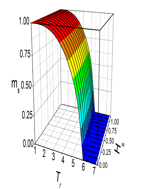
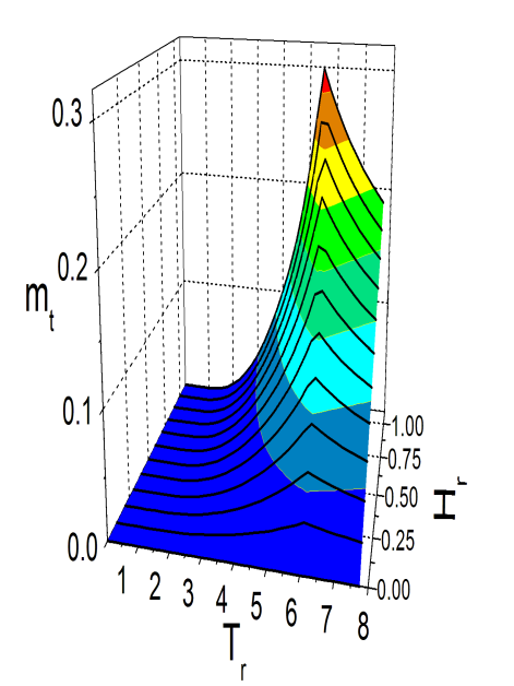
Figure 1: Variation of the antiferromagnetic (staggered) magnetization in the reduced field- reduced temperature plane for a second order phase transition.

Here, $\delta=J-J^{\prime}$, $t=J+J^{\prime}$, $z_{1}=2$ and $z_{2}=4$ . The metamagnetic spin-$1/2$ Ising model exhibits field-induced phase transitions. In Fig. 1(a) and (b) the variation of the antiferromagnetic and ferromagnetic order parameters are given in the field-temperature plane for a second order phase transition for $r=1.0$.

It has been shown in the extensive theoretical review by Kincaid and Cohen that metamagnetic Ising model exhibits different types of phase boundaries [20]. In this study, a Landau expansion of the free energy is performed and by a careful analysis of the signs of the coefficients, the possibility of different phase diagrams has been revealed. Further, Moreira et. al. has extended this analysis considering terms up to twelfth order [43]. The Landau expansion consists in developing the mean-field free energy given by Eq(4) in a power series of the order parameter ($m_{s}$) which vanishes near the critical point:

$$\Psi(T,H,m_{s})=\sum\limits_{k=0}^{n}\psi_{2k}(T,H)m_{s}^{2k}$$ (9)

According to the values and signs of the expansion coefficients one can distinguish different types of phase transitions: (i) For $\psi_{2}=0$ and $\psi_{4}<0$ and $\psi_{6}>0$ a first order transition appears. (ii) If $\psi_{2}=0$ and $\psi_{4}>0$ then an ordinary critical point takes place. (iii) For $\psi_{2}=0$ and $\psi_{4}=0$ and $\psi_{6}>0$ we experience tricritical point as a function of the ratio of the exchange interactions ($\eta=\frac{z_{2}J}{z_{1}J^{{}^{\prime}}}$):

$$\begin{array}[]{ccl}t_{TCP}&=&(1-\frac{1}{3\eta})\phi,\\ m_{TCP}&=&\sqrt{1-t_{TCP}},\\ h_{TCP}&=&\frac{1}{2}ln\frac{1+\sqrt{1-t_{TCP}}}{1-\sqrt{1-t_{TCP}}}+\frac{1-\eta}{1+\eta}\sqrt{1-t_{TCP}}\end{array}$$ (10)

where $\phi=z_{2}J+{z_{1}J^{{}^{\prime}}}$ and $t_{t}$ connects first and second order transition lines. On the other hand, for $r=0.3$ and $t=t_{TCP}$ $\psi_{2}=\psi_{4}=\psi_{6}=0$ which denotes a higher order critical point (TCP) [20, 43]. Consequently, topology of the metamagnetic Ising model phase diagram depends on the value of the ratio of the exchange interactions ($\eta=\frac{z_{1}J}{z_{2}J^{{}^{\prime}}}$): (i)If $r>0.3$, the transitions between the anti-ferromagnetic and paramagnetic phases are of first order at low temperatures and strong fields while it is of second order at higher temperatures. The two types of transitions are connected by a tricritical point. (ii) For $0<r<0.3$, the tricritical point decomposes into a critical end point (CEP) and a bicricital end point (BCP) with a line of first order transitions in between, separating two anti-ferromagnetic phases [20, 40], see Fig.7(a)-(b). The staggered magnetic susceptibility of an metamagnetic sytem is

$$\chi_{s}=\lim\limits_{H_{s_{r}}\rightarrow 0}\frac{\partial m_{s}}{\partial H_{s_{r}}}.$$ (11)

If one uses this definition and the equations of state given in Eq.(13), after some algebra the staggered magnetic can written as below

$$\chi_{s}=\lim\limits_{H_{s_{r}}\rightarrow 0}\frac{c_{2}a_{12}-a_{22}c_{1}}{a_{21}a_{12}-a_{22}a_{11}}.$$ (12)

Here, $H_{r}=H/{J}^{\prime}$ ,$H_{s_{r}}=H_{s}/{J}^{\prime}$ , $a_{11},a_{12},a_{21},a_{22},c_{1}$, and $c_{2}$ are given in Appendix A. Whereas direct magnetic susceptibility ($\chi_{\;t}$) is the response function of a system to a physical field and magnetic susceptibility can be expressed as,

$$\chi_{t}=\lim\limits_{H_{s_{r}}\rightarrow 0}\frac{\partial m_{t}}{\partial H_{r}}.$$ (13)

Following the similar steps we have used in obtaining staggered magnetic susceptibility, one obtains $\chi_{\;t}$ as

$$\chi_{t}=\lim\limits_{H_{s_{r}}\rightarrow 0}\{\frac{b_{22}d_{1}-b_{12}d_{2}}{b_{11}b_{22}-b_{12}b_{21}}\}.$$ (14)

3 Results

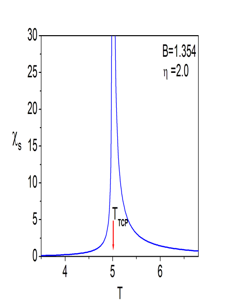
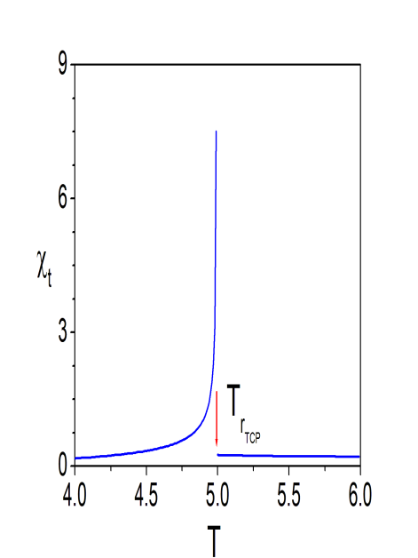
Figure 2: Behaviors of staggered (a) and magnetic (b) susceptibilities each as a function of reduced temperature for $H_{r}=\frac{H}{J^{{}^{\prime}}}=1.354$ and $r=J/J^{{}^{\prime}}=1.0.$ For these values, the system has a tricritical point (TCP). And also, staggered susceptibility increases rapidly with increasing temperature and diverges as the temperature approaches to the TCP.

Fig.2(a)-(b) represents the behavior of staggered and direct magnetic susceptibilities of spin-$1/2$ metamagnetic Ising model in the neighborhood of TCP for $r=1.0$. One can see from the figure that staggered susceptibility ($\chi_{s}$) increases rapidly with increasing temperature and diverges at the tricritical point. Whereas there is a discontinuity in the direct magnetic susceptibility ($\chi_{t}$) at the TCP. At this point we should note that $\check{Z}$ukovic et.al. has represented a study on dilute metamagnetic Ising Model within effective field theory [54, 55] which takes account the spin correlations. Comparing Fig.12 of Ref. [54] with Fig. 1(b) of the present Letter, one can see that our results are in accordance with the results of effective field theory. It’s important to note that, this behavior is in accordance with the existence of the discontinuity in $\chi_{t}$ on the critical curve, confirming that the transition there is second-order in the mean-field approximation [41] as well as effective field theory [54, 55]. On the other hand, Fig.3 illustrates the temperature variation of the tricritical direct magnetic susceptibility for various values of the ratio of the exchange interactions ($r$). One can see from this figure that the amplitude of the ferromagnetic susceptibility rises considerably high values for $r>1.78$. One of the characteristic behavior of the metamagnetic Ising model for strong anti-ferromagnetic case $(r<0.3)$ is the existence of the re-entrance phenomena. One can see this fact in the phase diagram of metamagnetic Ising model for $r>0.3$. For high values of the magnetic field the system is in a disordered state for $T_{r}\rightarrow 0$ whereas there is a transition from disorder to order at a finite temperature. In addition under goes another second order transition from ordered phase to disordered phase in high temperature regime ( see Fig.7(a) and (b)).

Fig.4(a) illustrates the temperature dependence of anti-ferromagnetic susceptibility for $H=H_{r_{DCP}}=1.994$ which corresponds to the double critical end point(DCP) of the spin-$1/2$ Ising model for $r=0.2$. Here $T_{r_{N_{1}}}$ at which staggered susceptibility diverges denotes the Neel temperature at which system undergoes a second order transition from paramagnetic phase to antiferromagnetic phase. Whereas the second divergence of the staggered susceptibility takes place at $T_{r_{DCP}}$. In addition one can clearly see that there exist an non-critical maximum at the ordered phase . This maximum corresponds to a anomaly in the multicritical behavior of iron group dihalides.

It is important to emphasize that Selke has reported that there is two lines of anomalies in the field-temperature phase diagram of the spin-$1/2$ Ising model with in mean field theory at which which the temperature derivative of the total magnetization exhibits, at fixed field value a maximum below the transition point, as exemplified in Fig. 3 of Ref.[40]. In this study the anomalies are related to the competing ordering tendencies of the external field and the interlayer couplings in a metamagnetic crystal. We should also note that there are experimental data which emphasizes the anomalies for quite some time [20]. In addition, there have been various experimental study on the field-induced Griffiths phase in Ising type metamagnets such as $FeBr_{2}$, $FeCl_{2}$ and $Fe_{1-x}Zn_{x}F_{2}$ [56, 57]. Fig.4(b) exhibits the temperature variation of ferromagnetic susceptibility for $H=H_{r_{DCP}}$. In this case the signature of the second order transition from paramagnetic phase to antiferromagnetic phase is a discontinuity in the direct magnetic susceptibility which is in accordance with the literature [41]. In addition, there exist a special multicritical point which separates the two different anti- ferromagnetic phases (AFI and AFII). This special continuous phase transition is of fourth order and direct magnetic susceptibility represents a discontinuity at the double critical end point. In addition direct susceptibility also represent a discontinuity at $T_{r_{N_{2}}}$ which corresponds to a regular critical point from antiferromagnetic phase to paramagnetic phase. Fig.6(a) shows the temperature dependencies of staggered and direct susceptibilities of the spin-$1/2$ metamagnetic system for $r=0.2$ and $H=H_{r_{CEP}}=1.99176$. At this value of the reduced physical magnetic field the system under goes two phase transitions of different character. The first transition is the CEP which is also of fourth order [20] and takes place between disordered phase at lower temperatures and anti ferromagnetic phase at higher temperature regime. One can easily observe from Fig.6 that the staggered susceptibility diverges at CEP whereas the direct magnetic susceptibility shows a discontinuity. Similar to the anomaly at $H=H_{r_{DCP}}$ , both $\chi_{\;t}$ and $\chi_{\;s}$ makes non-critical maximums in the antiferromagnetic phase. In Fig.6 (a) and (b) we have given the temperature variances of the magnetic response functions of the system for different constant reduced physical field values. One can see from these figures that the broad maximum in the ordered phase declines with decreasing the amplitude of the physical external magnetic field. Finally, the line of anomalies in the staggered and direct susceptibilities is depicted in Fig.7. Here $(T-H)_{\chi}$ denotes the field and temperature values which both the staggered and direct susceptibilities exhibit a broad maximum in the ordered phase as exemplified in Figs.4 and 5. Unlike the anomalies discussed by Selke the broad maximum does not diverges as one approaches the double critical endpoint. Further, the anomalies the magnetic response functions of the metamagnetic Ising system disappears for the case $r\geq 0.3$ where the critical end point and the double critical end points emerges to a tricritical point. In this case there is no re-entrance in the phase diagram.

4 Conclusions and Discussions

In this paper the magnetic response of iron group dihalides in a field with weak ferromagnetic intralayer interactions and highly coordinated antiferromagnetic interlayer couplings are studied within mean field approximation. The expressions that describe the staggered (anti- ferromagnetic) and direct (ferromagnetic) susceptibilities are derived by making use of mean field theory. The findings of this study can be summarized as follows: the direct susceptibility exhibits discontinuity not only at the second order transition point but also at multicritical points such as TCP, CEP, and DCP. In addition, the both magnetic response functions of the metamagnetic Ising model exhibits non-critical maximums in the ordered phase at the region of the $H_{r}-T_{r}$ in where the system shows re-entrance phenomena.

5 Acknowledgements

This work was supported by the Scientific and Technological Research Council of Turkey (TUBITAK), Grant No. 109T721. In addition authors thank A.N. Berker for valuable discussions, Sabanci University and Massachusetts Institute of Technology.

6 Appendix A

The coefficients $a_{11},a_{12},a_{21},a_{22},c_{1}$, and $c_{2}$ in Eq.(14) are defined as follows:

$$\begin{array}[]{lcl}a_{11}&=&1-\left(1-tanh\left(\frac{-2\left(m_{t}-m_{s}\right)+4r(m_{t}+m_{s})+H_{r}+H_{s_{r}}}{T_{r}}\right)^{2}\right)(2+4r)T_{r}^{-1},\\ \\ a_{12}&=&1-\left(1-tanh\left(\frac{-2(m_{t}-m_{s})+4r(m_{t}+m_{s})+H_{r}+H_{s_{r}}}{T_{r}}\right)^{2}\right)(-2+4r)T_{r}^{-1},\\ \\ a_{21}&=&-1+\left(1-tanh\left(\frac{-2(m_{t}+m_{s}+4r(m_{t}-m_{s})+H_{r}-H_{s_{r}}}{T_{r}}\right)^{2}\right)(2+4r)T_{r}^{-1},\\ \\ a_{22}&=&1-\left(1-tanh\left(\frac{-2(m_{t}+m_{s})+4r(m_{t}-m_{s})+H_{r}-H_{s_{r}}}{T_{r}}\right)^{2}\right)(-2+4r)T_{r}^{-1},\\ \\ c_{1}&=&\left(1-tanh\left(\frac{-2(m_{t}-m_{s})+4r(m_{t}+m_{s})+H_{r}+H_{s_{r}}}{T_{r}}\right)^{2}\right)T_{r}^{-1},\\ \\ c_{2}&=&\left(-1+tanh\left(\frac{-2(m_{t}+m_{s})+4r(m_{t}-m_{s})+H_{r}-H_{s_{r}}}{T_{r}}\right)^{2}\right)T_{r}^{-1},\\ \end{array}$$ (15)

7 Appendix B

The coefficients $b_{11},b_{12},b_{21},b_{22},d_{1}$, and $d_{2}$ in Eq.(14) are defined as follows:

$$\begin{array}[]{lcl}b_{11}&=&1-\left(1-tanh\left(\frac{-2(m_{t}-m_{s})+4r(m_{t}+m_{s})+H_{r}+H_{s_{r}}}{T_{r}}\right)^{2}\right)(2+4r)T_{r}^{-1},\\ \\ b_{12}&=&1-\left(1-tanh\left(\frac{-2(m_{t}-m_{s})+4r(m_{t}+m_{s})+H_{r}+H_{s_{r}}}{T_{r}}\right)^{2}\right)(-2+4r)T_{r}^{-1},\\ \\ b_{21}&=&-1+\left(1-tanh\left(\frac{-2(m_{t}+m_{s})+4r(m_{t}-m_{s})+H_{r}-H_{s_{r}}}{T_{r}}\right)^{2}\right)(2+4r)T_{r}^{-1},\\ \\ b_{22}&=&1-\left(1-tanh\left(\frac{-2(m_{t}+m_{s})+4r(m_{t}-m_{s})+H_{r}-H_{s_{r}}}{T_{r}}\right)^{2}\right)(-2+4r)T_{r}^{-1},\\ \\ d_{1}&=&\left(1-tanh\left(\frac{(-2(m_{t}-m_{s})+4r(m_{t}+m_{s})+H_{r}+H_{s_{r}})}{T_{r}}\right)^{2}\right)T_{r}^{-1},\\ \\ d_{2}&=&\left(1-tanh\left(\frac{(-2(m_{t}+m_{s})+4r(m_{t}-m_{s})+H_{r}-H_{s_{r}})}{T_{r}}\right)^{2}\right)T_{r}^{-1}.\end{array}$$ (16)

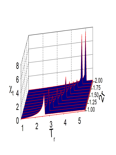
Figure 3: The temperature variation of the tricritical direct magnetic susceptibility for various values of the ratio of the exchange interactions. Here the arrows illustrate the phase transition temperatures.

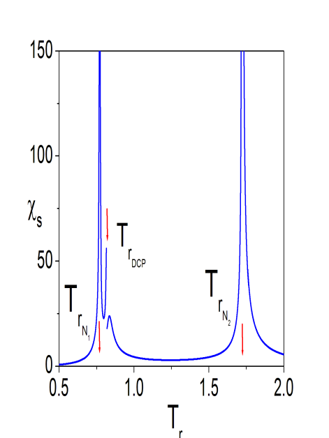
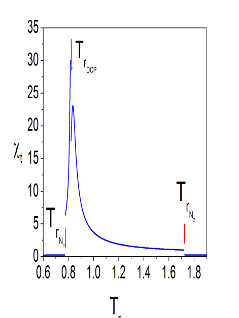
Figure 4: The temperature dependencies of staggered and total susceptibilities in the neighborhood of double critical point (DCP) and second order phase transition point which takes place for the value of the reduced magnetic field $H_{r_{DCP}}=1.994$ for $r=0.2$. Here the arrows illustrate the phase transition temperatures.

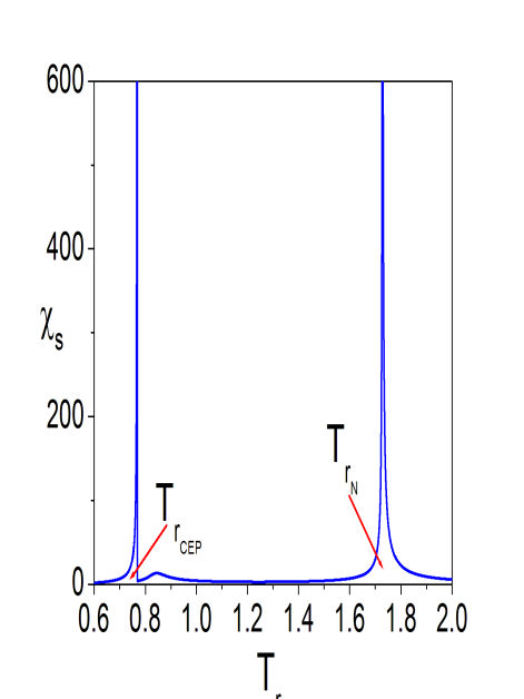
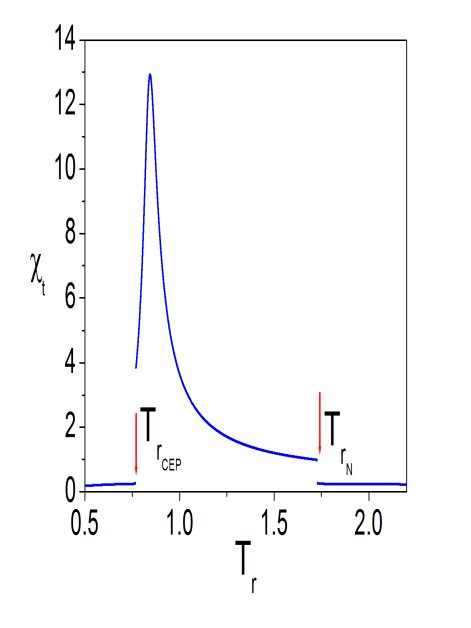
Figure 5: The temperature dependencies of staggered and total susceptibilities in the neighborhood of the critical end point (CEP) and second order phase transition point which takes place for the value of the reduced magnetic field $H_{r_{CEP}}=1.99176$ for $r=0.2$. Here the arrows illustrate the phase transition temperatures.

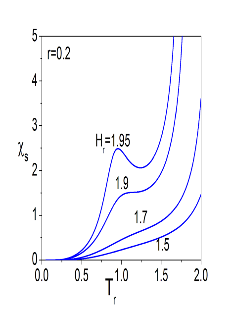
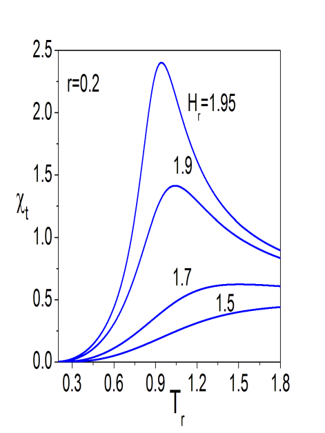
Figure 6: The behavior of (a) the staggered susceptibility $\chi_{s}$ (b) the direct magnetic susceptibility $\chi_{t}$ as a function of the reduced temperature, where $T_{r}=\frac{k_{B}T}{J^{{}^{\prime}}}$ is for several values of reduced field, $H_{r}=\frac{H}{J^{{}^{\prime}}}$.

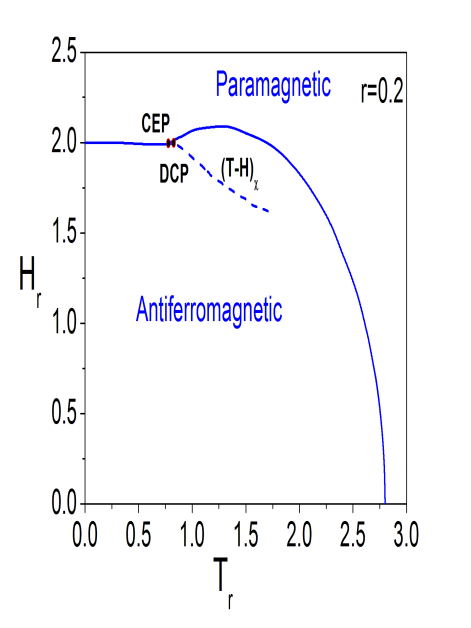
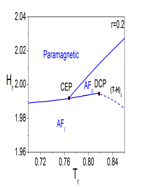
Figure 7: The calculated mean field phase diagram of the metamagnetic Ising model for $r=\frac{J}{J^{{}^{\prime}}}=0.2$ in the temperature- field plane. (b) Detailed phase diagram in the neighborhood of the critical end point (CEP) and the double critical end point (DCP). The dashed lines denote the anomalies in the staggered and direct susceptibilities.

References

- [1] V. Taufour, D. Aoki, G. Knebel, and J. Flouquet, Phys. Rev. Lett. 105 (2010) 217201.
- [2] A. Hankey, T. S. Chang, and H. E. Stanley, Phys. Rev.A 9 (1974) 2573.
- [3] B. Ginzberg; S. Bergerman; D. H. Kurlat, Phys. and Chem. of Liq. 27 (1994) 83.
- [4] C. W. Garland and B. B. Weiner, Phys. Rev.B 3 (1973) 1634.
- [5] E. K. Riedel, Phys. Rev. Lett. 28 11 (1972).
- [6] P. S. Peercy, Phys. Rev. Lett. 35 (1975) 1581 ; V. H. Schmidt, Bull. Am. Phys. Soc. 19 (1974) 649.
- [7] R. Leidl, H. W. Diehl, Phys. Rev. B 57 (1998) 1908.
- [8] M. Iwata, Z. Kutnjak, Y. Ishibashi, and R. Blinc, J. Phys. Soc. Jpn. 77 (2008) 065003.
- [9] P. H. van Konynenburg and R.L. Scott, Philos. Trans. R. Soc. Ser. A 298 (1980) 495.
- [10] L. Demko, I. Kezsmarki, G. Mihaly, N. Takeshita, Y. Tomioka, and Y. Tokura, Phys. Rev. Lett. 101 (2008) 037206.
- [11] M. Kaufman, P.E. Klunzinger, A. Khurana, Phys. RevB. 34 (1986) 4766 .
- [12] W. Selke, Z. Phys. B 101 (1996) 145.
- [13] N. B. Wilding, Phys. Rev. Lett. 78 (1997) 1488.
- [14] M. E. Fisher and P.J. Upton, Phys. Rev. Lett. 65 (1990) 2402; 65 (1990) 3405.
- [15] M. E. Fisher and M.C. Barbosa, Phys. Rev. B 43 (1991) 11177; 43 (1991) 10635.
- [16] M. C. Barbosa, Phys. Rev. B 45 (1992) 5199.
- [17] W. Poot and T.W. de Loos, Phys. Chem. Chem. Phys. 1 (1999) 4923.
- [18] W. P. Wolf, Braz. J. Phys. 30 (2000) 794.
- [19] K. Katsumata, H. Aruga Katori, S.M. Shapiro, and G. Shirane, Phys. Rev. B 55 (1997) 11466.
- [20] J. M. Kincaid and E. G. D. Cohen, Phys. Reports C 22 (1975) 57.
- [21] E. Stryjewski and N. Giordano, Adv. Phys. 26 (1977) 487.
- [22] Y.-L. Wang and J.D. Kimel, J. Appl. Phys. 69 (1991) 6176.
- [23] J. D. Kimel, S. Black, P. Carter, and Y.-L. Wang, Phys. Rev. B 35 (1987) 3347.
- [24] J. A. Plascak and D. P. Landau, Phys. Rev. E 67 (2003) 015103R .
- [25] V. A. Alessandrini, H.J. de Vega, and F. Schaposnik, Phys. Rev.B. 12 (1975) 5034 .
- [26] D. P. Landau, Phys. Rev.B 14 (1976) 4054 .
- [27] D. P. Landau and M.E. Fisher, Phys. Rev.B 11, 1030 (1975); ibid. 12 (1975) 263.
- [28] M. Barkowiak, J.A. Henderson, J. Oitmaa, P.E. de Brito, Phys. Rev.B 51 (1995) 14077 .
- [29] W. Li, S.-S.Gong, Y. Zhao, S.-J. Ran, S. Gao, and G. Su, Phys. Rev. B 82 (2010) 134434 .
- [30] Z. He and Y. Ueda, Phys. Rev. B 77 (2008) 052402.
- [31] A. J. Millis, C. Lampropoulos, S. Mukherjee, and G. Christou, Phys. Rev. B, 82 (2010) 174405 .
- [32] E. Stryjewski, M. Giordano, Adv. Phys. 26 (1977) 487.
- [33] H.D. Zhou, E. S. Choi, Y.J. Jo, L. Balicas, J. Lu, L. L. Lumata, R. R. Urbano, P. L. Kuhns, A. P. Reyes, J. S. Brooks, R. Stillwell, S. W. Tozer, C.R. Wiebe, J. Whalen, and T. Siegrist, Phys. Rev.B 82 (2010) 054435 .
- [34] V. M. Kalita, A. F. Lozenko, S. M. Ryabchenko, and P. A. Trotsenko, Low Temp. Phys. 31 (2005) 794.
- [35] T. Fujita, A. Ito and K. no, J. Phys. Soc. Jpn, 27 (1969) 1143.
- [36] D. P. Landau, Phys. Rev. Lett. 28 (1972) 449.
- [37] B. L. Arora, D. P. Landau, AIP Conf. Proc. 10 (1973) 870.
- [38] F. Harbus, H. E. Stanley, Phys. Rev. B 8 (1973) 1156.
- [39] F. Harbus, H. E. Stanley, Phys. Rev. B 8 (1973) 1141.
- [40] W. Selke, Z. Phys. B 101, 145 (1996).
- [41] D. A. Lavis, G. M. Bell, Statistical Mechanics of Lattice Systems 1, Berlin, Springer, (1999).
- [42] G. Gulpinar, D. Demirhan, F. Buyukkilic, Phys. Rev. E 75, (2007) 021104.
- [43] A. F. S. Moreira, W. Figueiredo, and V. B. Henriques, Eur. Phys. J. B. 27, (2002) 153.
- [44] L. Hernandez, H. T. Diep, D. Bertrand, Phys. Rev. B 47 (1993) 2602.
- [45] Z. Onyszkiewicz, A. Wierzbicki, Physica B 151 (1988) 462.
- [46] Z. Onyszkiewicz, A. Wierzbicki, Physica B 151 (1988) 475.
- [47] M. James, J. Phys. Chem. Solids 61 (2000) 1865.
- [48] W. Kleemann, H. A. Katori, T. Kato, Ch. Binek, K. Katsumata, Europhys. Lett. 55 (2001) 732.
- [49] H. A. Katori, K. Katsumata, O. Petracic, W. Kleemann. T. Kato, Ch. Binek, Phys. Rev. B 63 (2001) 132408.
- [50] Y. Narumi, K. Katsumata, T. Nakumura, Y. Tanaka, S. Shimomura, T. Ishikawa, M. Yabashi, J. Phys.: Condens. Matter 16 (2004) L57.
- [51] P. E. Engelstad and K. Yamada, Phys. Rev. B 52 (1995) 13029.
- [52] G. Durin, M. Bonaldi, M. Cerdonio, R. Tommasini, S. Vitale, J. Magn. Magn. Mater. 101 (1991) 89.
- [53] M. B. F. van Raap, F.H. Sanchez, C.E.R. Torres, L. Casas, A. Roig, E. Molins, J. Phys.: Condens. Matter 17 (2005) 6519.
- [54] M. Zukovic, A. Bobak ve T. Idogaki, J. Magn. Magn. Mater. 188 (1998) 52.
- [55] M. Zukovic, A. Bobak ve T. Idogaki, J. Magn. Magn. Mater. 192 (1999) 363.
- [56] Ch. Binek, W. Kleemann, Phys. Rev. Lett. 72 (1994) 1287; Ch. Binek, W. Kleemann, Acta Phys. Slovaca 44 (1994) 435.
- [57] Ch. Binek, M.M.P. de Azedevo, W. Kleemann, D. Bertrand, J. Magn. Magn. Mater. 140 144 (1995) 1555.