On the Alfred Gray’s Elliptical Catenoid

Abstract

We give a parameterization, using Jacobi’s elliptic functions, of Alfred Gray’s Elliptical Catenoid and Elliptical Hellicoid that avoids some problems present in the original depiction of these surfaces.

1 Introduction: The Björlings problem

On of the Alfred Gray’s favorite tools was the solution to Björling’s problem: Given a planar analytic curve, find a minimal surface in $\mathbb{R}^{3}$ that contains it as a geodesic. The Weierstrass representation provides an explicit solution: if $(x(t),y(t))$ is a parameterization of the curve, the parameterization

$$\Phi(z)=\Re\left(x(z),y(z),i\int_{p}^{z}\sqrt{x^{\prime}(u)^{2}+y^{\prime}(u)^{2}}du\right)$$ (1)

gives the solution, where $x(z)$, $y(z)$ are extensions of $x(t)$, $y(t)$ to functions of a complex variable $z$. We will call it the Björling surface of the curve. When one takes, instead of the real part, the imaginary part of the expression, one gets another minimal surface, known as the conjugated surface of the first one.

It is well know how Alfred used this to produce many beautiful surfaces. But he could use it also as a theoretical tool: one day we asked Alfred what order of contact could a minimal surface have at a self-intersection point; without a second of thought he replied: “Any order of contact: take a planar curve with a self-contact of order $n$ and solve Björling’s problem”. An instant theorem!.

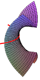
Figure 1: The wrong picture for the parabola’s Björling.

Formula (1) can be directly given to the computer. However, the fact that the integrand is in many cases multivaluated poses some problems when we try to get the global picture. Take, for instance, the parabola $(2t,t^{2})$. The formula gives the following parameterization of its Björling surface

$$\Phi(z) = \Re\left(2z,z^{2},i\int_{0}^{z}\sqrt{1+u^{2}}du\right)$$

which the reader can immediately give to his favorite graphics package…and get the wrong picture! (Figure 1a, where the thick line shows the parabola). The problem has to do with the integrand that is multivalued and branches at the points $i$ and $-i$. When we integrate from 0 to, say, $2i$ along differents paths we can get different values, all with the same imaginary part. This produces a sharp edge, which is impossible in a minimal surface. The problem is more evident in the conjugate surface: we get a discontinuity which the computer fills with a planar face (Figure 1b).

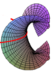
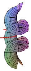
(a) Two views of Catalan’s surface.

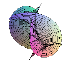
(b) The conjugate surface.

Figure 2: The right picture for the parabola’s Björling.

The problem can be easily solved by a simple sustitution $z=sinhw$ which makes the function single valued and the surface becomes:

$$\Phi(w)=\Re\left(2\sinh(w),\sinh^{2}(w),2i\cosh(w\sinh(w))+w\right)$$

which gives the correct picture (Figure 2). The surface continues beyond the sharp edges which becomes lines of self-intersection and then takes a turn, giving a periodic pattern. The surface turns out to be the well-know Catalan’s surface that contains a cycloid perpendicular to the parabola which is another planar geodesic of the surface. Figure 2b shows the correct conjugate surface.

2 Björling’s duality

The above relation shows an interesting relation between the parabola and the cycloid: they have the same Björling surface. Recall that a plane cuts a minimal surface along a geodesic, if and only if, it is a plane of symmetry of the surface. Now, the Björling surface of a curve that has a line of symmetry has to planes of symmetry: the original one containing the curve and the plane perpendicular to it that contains the line of symmetry. In formula (?) the original curve is obtained by restricting to real values of $z$ and the orthogonal geodesic by restricting to purely imaginary values of $z$. The two curves are in a sense, dual to each other. To be more precise: The duality is between objects consisting each of a curve and a point of intersection of the curve with a line of symmetry. We can call those pairs Björling duals to each other. For example, the circle and the catenary are Björling duals (the common surface is the catenoid) and so are the parabola and the cycloid with its line of symmetry that cuts t on one of the highest (smooth) points of the cycle.

3 The Elliptical Catenoid

Let us apply (1) to the ellipse with semi-axes $a$ and $b$ $a>b$, and excentricity $e=\frac{\sqrt{a^{2}-b^{2}}}{b}$. We obtain

$$\Phi(z) = \Re\left(b\cos(z),a\sin(z),i\int_{0}^{z}\sqrt{1-e^{2}\sin^{2}(u)}du\right)$$ (2)

and with it the computer produces Figure 3. One observes that this surface has various channels where one of the principal curvatures is close to zero and the other one is very big. Again, this cannot be a minimal surface! (One obtains a channel or an edge depending on the parity of the size of the grid used to plot the surface). The conjugate surface presents again a discontinuity which if filled by the computer with a flat face (Figure 3b)

Alfred’s depiction in [1] of these surfaces, called by him Elliptical Catenoid and Elliptical Hellicoid, have the same problems. (Those two loves of his, the computer and the Björling problem, did not get togheter as smoothly as he thought). Both Maple (which we use) and Mathematica give the same picture. Maybe Alfred was aware of the problem since in this case he used an elliptic function instead of applying directly the formula. The analysis must, however, be carried some steps further:

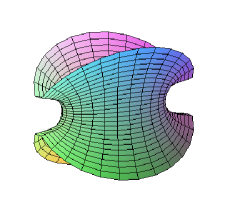
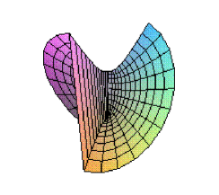
Figure 3: The bad picture for the Elliptical Catenoid.

We use Jacobi’s elliptic functions (for details, see [2], [3]): Jacobi’s elliptic sine function $\phi={\rm sn}(v,k)$, being the inverse function of the integral

$$v=\int_{0}^{\phi}\frac{dt}{\sqrt{1-t^{2}}\sqrt{1-k^{2}t^{2}}},$$

Jacobi’s elliptic cosine

$${\rm cn}(v,k)=\sqrt{1-{\rm sn}^{2}(v,k)}$$

and Jacobi’s delta function

$${\rm dn}(v,k)=\sqrt{1-k^{2}{\rm sn}^{2}(v,k)}.$$

Like the trigonometric funtions (which we obtain as the particular case $k=0$) they can be extended to complex functions, but the extensions are now meromorphic and doubly periodic instead of being holomorphic and periodic.

With the new parameter $u$ related to $z$ by ${\rm sn}(u,e)=\sin(z)$ we obtain the parameterization:

$$\ Psi(u)=\Re\left(b{\rm cn}(u,e),a{\rm sn}(u,e),ia\int_{0}^{u}{\rm dn}^{2}(\sigma,e)d\sigma\right).$$

The integrand is still a meromirphic function, but its residues are all $0$ [2, p.241], so the integral is a well-defined function of $u$. This parameterization produces the correct picture of the Elliptical Catenoid. The ellipse has two lines of symmetry and, correspondly, two Björling duals: one resembles a cycloid, the other one a catenary. Figure 4 shows the correct pictures of the Elliptical Catenoid and the Elliptical Hellicoid:

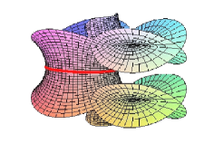
(a) The Elliptical Catenoid.

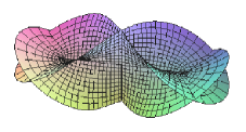
(b) The conjugate surface.

Figure 4: The right picture for the Elliptical Catenoid.

The same method gives the Björling surface of the hyperbola (where now we take $k=\frac{1}{e}<1$):

$$\ Psi(u)=\Re\left(b{\rm dn}(u/k,k),iak{\rm sn}(u/k,k),a\int_{0}^{u}{\rm cn}^{2}(\sigma/k,k)d\sigma\right).$$

The dual curve of the hyperbola again resembles a cycloid.

The analysis of the björling surfaces of the conics will be developed fully in a forthcoming article.

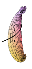
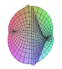
Figure 5: The Björling surface for the hyperbola and its conjugated.

References

- [1] A. Gray, Modern Differential Geometry of Curves and Surfaces, CRC Press, 2nd Edition, 1998.
- [2] D. F. Lawden, Elliptic Functions and Applications, Applied Mathematical Sciences 98, Springer-Verlag, 1989.
- [3] A.I. Markusevich, The Remarkable Sine Functions, Elsevier, 1966.