Magnetostatic bias in multilayer microwires: theory and experiments

Abstract

The hysteresis curves of multilayer microwires consisting of a soft magnetic nucleus, intermediate non-magnetic layers, and an external hard magnetic layer are investigated. The magnetostatic interaction between magnetic layers is proved to give rise to an antiferromagnetic-like coupling resulting in a magnetostatic bias in the hysteresis curves of the soft nucleus. This magnetostatic biasing effect is investigated in terms of the microwire geometry. The experimental results are interpreted considering an analytical model taking into account the magnetostatic interaction between the magnetic layers.

I Introduction

During the last decade, soft magnetic materials have been deeply investigated. Besides the basic scientific interest in their magnetic properties, there is a great deal of technologic interest due to their use in sensing applications, particularly in the fields of automotive, mobile communication, medical and home appliance industries. Vazquez07 ; CTD+04 ; MH07 ; KMP03 Moreover, these materials are very promising for spintronic devices in magnetic recording media. YKN+07 Two types of soft magnetic microwire families are currently studied: in-water quenched amorphous wires with diameters of around 120 $\mu$m, OU95 and quenched and drawn microwires with diameters ranging from around 2 to 20 $\mu$m, ZGV+03 covered by a protective insulating glassy coat. The most interesting magnetic property observed in these ultrasoft magnetic microwires is a single Barkhausen jump that results in a square-shaped hysteresis loop found in Fe-based microwires, as a consequence of magnetization reversal by displacement of a single domain wall. VGV05 The development of preparation techniques had lead to the production of well controlled multilayered systems composed by layers of different materials. In particular, magnetic multilayers have been grown, like magnetic/nonmagnetic trilayers and multisegmented wires. Virtually all the multilayer magnetic systems present magnetostatic bias effects as a consequence of the coupling between adjacent layers with different magnetic character. In such systems, the low-field hysteresis loops are shifted along the field direction by an amount which is labeled as magnetostatic bias field, $H_{b}$. In fact, the magnetostatic bias field acts as an additional magnetic field on the layer that magnetizes at lower fields, being equivalent to an unidirectional magnetic anisotropy. The role played by magnetic biasing in controlling the magnetization reversal in heterostructures is a key issue for applications related to spin electronic devices and ultrahigh density recording media. In fact, this is in the base of spin-valve and magnetic tunnel junction’s heads where magnetic exchange coupling between ferromagnetic (FM) and antiferromagnetic (AFM) layered structures facilitates the material to exhibit a well defined non-symmetric response to magnetic excitations. NS99

In the last years, a family of multilayer microwires has been introduced by Pirota et al. PHN+04 in which quenching and drawing, sputtering and electroplating techniques have been combined to prepare multilayer microwires consisting of two metallic layers separated by an intermediate insulating microlayer: a micrometric cylindrical nucleus with a radius $R_{i}$ and an external metallic outer microtube with internal and external radii $a_{e}$ and $R_{e}$, respectively. The length of the microwire is $L$. In order to simplify the illustration of our results, we present figures in terms of $R_{i}$, $t_{s}$ and $t_{e}$, where $t_{s}=a_{e}-R_{i}$ is the thickness of the intermediate non-magnetic spacer layer and $t_{e}=R_{e}-a_{e}$ represents the thickness of the external microtube, as illustrated in Fig. 1(a).

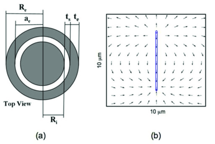
Figure 1: (a) Geometrical parameters of the cross section of the multilayer microwire. (b) Magnetostatic field profile for a tube uniformly magnetized with $L=6$ mm, $R_{e}=25$ $\mu$m and $a_{e}=20.8$ $\mu$m.

Due to the geometry, the magnetization of the complete microwire should be strongly influenced by the magnetostatic interaction between the nucleus and the external microtube. As a consequence, a shift of the low-field hysteresis loop is expected to appear, which is not related to any kind of exchange NS99 ; STZ+03 but rather to magnetostatic biasing effect. The possibility to achieve such spin-valve-like hysteresis loop is very attractive for its applications to sense magnetic fields in magnetic recording systems.

Although the magnetic behavior of multilayer microwires has been intensely investigated experimentally, VBK+07 ; TKP+07 ; TBP+07 analytical calculations of the magnetostatic interaction between the magnetic layers have not yet been performed. Our intention is to fill this gap by proposing a simple model for the magnetostatic interaction in a multilayer microwire. From the derived interaction energy we obtain a magnetostatic bias field that can be directly compared to experimental results. Furthermore the analytical result is generalized for a broad range of geometrical parameters.

II Experimental Details

Multilayer magnetic microwires have been prepared with suitable composition and characteristics to obtain optimized soft/hard multilayer system so that inter-layer magnetostatic interaction can be properly detected. A detailed description of the fabrication technique can be found elsewhere. ZGV+03 ; PHN+04 The precursor microwire investigated consists of an amorphous nucleus ($R_{i}=8.7$ $\mu$m) with nominal composition Co_67.06Fe_3.84Ni_1.44B_11.53Si_14.47Mo_1.66. For this alloy composition a balanced magnetostriction of the order of $10^{-7}$ is reached, resulting in an ultrasoft magnetic behavior. This soft nucleus is coated by an intermediate non-magnetic Pyrex layer ($t_{s}=12.1$ $\mu$m thick) produced by the quenching and drawing method. ZGV+03 Then, a 30 nm thick Au nanolayer is sputtered onto the Pyrex coating, which plays the role of electrode/substrate for the final electroplating of the magnetically harder CoNi outer microlayer. The thickness of the CoNi layer depends on the current density and the electroplating time, while the relative amount of Co and Ni slightly varies with the current density. PPG+05 In the present study, the electroplating was performed at 40 ^∘C at fixed current density of 6 mA/cm² during a time that was varied up to 60 min. A thickness growth ratio of 0.28 $\mu$m/min for the electroplated shell has been determined by Scanning Electron Microscopy. The composition of the magnetic external shell was Co₉₀Ni₁₀, with a saturation magnetization $M_{e}^{0}=1.2\times 10^{6}$ A/m as determined by XR fluorescence. A relatively hard magnetic behavior is found for this external shell.

The magnetic properties have been determined in a VSM and inductive magnetometer at the temperatures 5 and 300 K with the applied magnetic field parallel to the microwire axis. Two series of hysteresis loops have been measured: (i) high-field loops ($\pm 40$ kA/m maximum applied field) to analyze the magnetic behavior of the multilayer microwire, and (ii) low-field loops ($\pm 1$ kA/m maximum field) measured after premagnetazing under a nearly saturating field of $\pm 80$ kA/m to obtain information about the magnetostatic interaction between different layers. Such magnetostatic coupling has been analyzed as a function of the dimensions of the hard layer: thickness and length, respectively. All samples were carefully measured in the same position and orientated with the North magnetic pole, where the terrestrial field is well known and it is removed after the measurements.

III Theoretical calculations

Our model system consists of a microtube made of a hard magnetic material with magnetization saturation $M_{e}^{0}$, containing in its interior a soft magnetic cylindrical nucleus with saturation magnetization $M_{i}^{0}$. We adopt a simplified approach in which the discrete distribution of magnetic moments of both nucleus and tube is replaced by a continuous one, defined by a function $\mathbf{M}(\mathbf{r})$ such that $\mathbf{M}(\mathbf{r})\delta V$ gives the total magnetic moment within the element of volume $\delta V$ centered at $\mathbf{r}$. We consider wires for which $L\gg R_{e}$ so it is reasonable to assume an axial magnetization due to shape anisotropy, defined by $\mathbf{M}(\mathbf{r})=M_{0}\mathbf{\hat{z}}$, where $\mathbf{\hat{z}}$ is the unit vector parallel to the wire axis. The magnetostatic interaction between the nucleus and the microtube can be calculated from Aharoni

$$E_{int}=\mu_{0}\int\mathbf{M}_{i}(\mathbf{r})\nabla U_{e}(\mathbf{r})\,dV\ ,$$

where $\mathbf{M}_{i}(\mathbf{r})$ is the magnetization of the nucleus and $U_{e}(\mathbf{r})$ is the magnetostatic potential of the external microtube. The expression for this potential has been previously reported EAA+08 and is given by

$$U\left(r,z\right)=\frac{M_{e}^{0}}{2}\int_{0}^{\infty}\frac{dk}{k}J_{0}\left(kr\right)\\ \left[R_{e}J_{1}\left(kR_{e}\right)-a_{e}J_{1}\left(ka_{e}\right)\right]\\ \left(e^{-k\left|\frac{L}{2}-z\right|}-e^{-k\left|-\frac{L}{2}-z\right|}\right)$$ (1)

From (1) it is possible to obtain the expression for the magnetostatic field. Thus we write, $\mathbf{H_{e}}\left(r,z\right)=-\nabla U_{e}=H_{r}\left(r,z\right)\mathbf{\hat{r}}+H_{z}\left(r,z\right)\mathbf{\hat{z}}$ with

$$H_{r}\left(r,z\right)=\frac{M_{e}^{0}}{2}\int_{0}^{\infty}dk\left[R_{e}J_{1}\left(kR_{e}\right)-a_{e}J_{1}\left(ka_{e}\right)\right]\\ J_{1}\left(kr\right)\left(-e^{-k\left|\frac{L}{2}-z\right|}+e^{-k\left|-\frac{L}{2}-z\right|}\right)$$

and

$$H_{z}\left(r,z\right)=\frac{M_{e}^{0}}{2}\int_{0}^{\infty}dk\left[R_{e}J_{1}\left(kR_{e}\right)-a_{e}J_{1}\left(ka_{e}\right)\right]\\ J_{0}\left(kr\right){\LARGE(}\mbox{sign}\left(\frac{L}{2}-z\right)e^{-k\left|\frac{L}{2}-z\right|}\\ -\mbox{sign}\left(-\frac{L}{2}-z\right)e^{-k\left|-\frac{L}{2}-z\right|}{\LARGE)}$$

Figure 1(b) illustrates the magnetostatic field profile for a tube with $L=6$ mm, $a_{e}=20.8$ $\mu$m and $R_{e}=25$ $\mu$m.

Finally, the magnetostatic interaction between the two magnetic layers in the microwire is given by

$$E_{int}=\pi\mu_{0}M_{i}^{0}M_{e}^{0}R_{i}R_{e}\int\limits_{0}^{\infty}\frac{dk}{k^{2}}J_{1}(kR_{i})\\ \left(J_{1}(kR_{e})-\frac{a_{e}}{R_{e}}J_{1}(ka_{e})\right)\left(1-e^{-kL}\right)\ ,$$

where $J_{1}$ is a Bessel function of first kind and first order.

The coercivity, $H_{c}$, of a soft magnetic nucleus in the multilayer microwire can be calculated as

$$H_{c}=H_{c}^{i}-H_{b}\ ,$$

where $H_{c}^{i}$ is the coercivity of the soft magnetic nucleus if isolated and $H_{b}$ is the magnetostatic bias field due to the magnetostatic interaction between the external hard magnetic shell on the soft magnetic nucleus. This magnetostatic bias field can be written as a function of the magnetostatic interaction between the magnetic layers

$$H_{b}=\frac{E_{int}}{\mu_{0}M_{i}^{0}V}\ .$$ (2)

IV Results

Figure 2 shows the high-field hysteresis loop for a multilayer microwire with $t_{e}=4$ $\mu$m at room temperature. As observed, the magnetization process takes place in two steps: a giant Barkhausen jump in very low field, of a few A/m, that must be ascribed to the magnetic amorphous nucleus; and an additional spread jump (in the range between $10$ and $20$ kA/m), corresponding to the harder CoNi outer shell. The flat region before the second step is reversible until a field of $3$ kA/m. At higher fields an irreversible contribution appears. The fractional magnetization jump and the effective coercivity of the loop depend on the thickness and composition of the hard shell. PPG+05 ; TBP+07

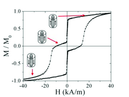
Figure 2: High-field hysteresis loop for a soft/hard multilayer microwire with a thickness of the outer hard magnetic layer $t_{e}=4$ $\mu$m.

As observed in Fig. 2, the loop is symmetrical, indicating that no relevant interaction between magnetic layers is present. To investigate the magnetostatic biasing effect in the multilayer microwires, the low-field hysteresis loops of the composite microwire have been analyzed. Previous to these low-field measurements, the microwires were premagnetized under a nearly saturating dc magnetic field. The study is then performed under maximum applied fields smaller than the one required to reverse the magnetization of the hard outer shell, in order that only the internal nucleus contributes to the hysteresis loops.

IV.1 Dependence of the thickness of the CoNi microtube on the dipolar bias

Figure 3 shows the low-field loop for wires with $L=6$ mm, $R_{i}=8.7$ $\mu$m and $t_{s}=12.1$ $\mu$m, considering different values of thickness, $t_{e}$, of the outer microtube, measured after premagnetization at $\pm 80$ kA/m.

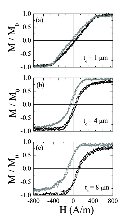
Figure 3: Low-field hysteresis loops for composite microwires with $L=6$ mm, $R_{i}=8.7$ $\mu$m and $t_{s}=12.1$ $\mu$m, after premagnetizing at $+80$ kA/m (black dots illustrate both branches of the cycle) and $-80$ kA/m (gray dots illustrate both branches of the cycle) for a CoNi thickness of (a) $t_{e}=1$ $\mu$m, (b) $t_{e}=4$ $\mu$m and (c) $t_{e}=8$ $\mu$m.

It should be emphasized that the premagnetazing process is needed in order to observe the magnetostatic biasing effect, that is, the shift of the loops towards the orientation of the premagnetizing field. With this process the hard layer remains practically at its remanence state, creating a fixed non-homogeneous magnetic field at the soft nucleus of the multilayer microwire. The sign of this magnetic field depends on the orientation of the premagnetizing field. When the outer shell is positively magnetized the field it produces in the nucleus region is basically negative, thus shifting the hysteresis loop towards positive values as confirmed in Fig. 3. This shift is consistent with the definition of the magnetostatic bias field, $H_{b}$, and is similar to the one due to exchange coupling in FM/AFM bilayers. Since exchange coupling can be discarded due to the thickness of the intermediate non-magnetic layers, the coupling must be of magnetostatic origin. Moreover, the presence of the premagnetized hard outer shell introduces another asymmetry behavior in the magnetization curve of the soft layer, that is, a second magnetization region with lower susceptibility appears at higher positive or negative field according with positive or negative premagnetization, respectively. Such asymmetric behavior is due to the inhomogeneity of the magnetostatic bias field. The magnetic volume of the second magnetization region increases with the CoNi thickness as shown in figure 3 in Ref. 14. The previously study of magnetization profiles in trilayer ribbons with the same magnetic configuration (CoNi/CoFeSiB/CoNi), has proved that the second magnetization region with low susceptibility is found close to the uncompensated poles of the hard layer, where the magnetostatic bias field is stronger. TKB+08

Theoretical and experimental magnetostatic results are combined in Fig. 4. Experimental data for the magnetostatic bias field for different values of the hard layer thickness are depicted by gray dots and the theoretical prediction is represented by the solid line. It is clear that there is a strong dependence of the bias field on $t_{e}$. Note the good agreement between experimental datapoints and analytical results for multilayer microwires for $t_{e}<10$ $\mu$m.

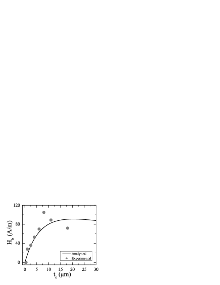
Figure 4: Magnetostatic bias field as a function of the thickness of the CoNi layer. The gray dots correspond to experimental data and the solid line represents the values calculated analytically. Parameters: $L=6$ mm, $R_{i}=8.7$ $\mu$m and $t_{s}=12.1$ $\mu$m. We have used $M_{e}^{0}=1.2\times 10^{6}$ A/m.

IV.2 Dependence of the bias field on the microwire length

Figure 5 shows the low-field loop for wires of $t_{e}=11$ $\mu$m, $R_{i}=8.7$ $\mu$m and $t_{s}=12.1$ $\mu$m, and different lengths, $L$, measured after premagnetizing at $\pm 80$ kA/m. The shape of the shifted loops notably depends on the length of the samples. With increasing length, the loops become asymmetric and the magnetostatic bias field is reduced. For longer length, the loops become again symmetric. Further analysis of this evolution with length is performed elsewhere. TKP+07 ; TBP+07

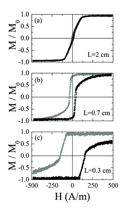
Figure 5: Low-field hysteresis loops for composite microwires of $t_{e}=11$ $\mu$m, $R_{i}=8.7$ $\mu$m and $t_{s}=12.1$ $\mu$m, after premagnetizing at $+80$ kA/m (black dots illustrate both branches of the cycle) and $-80$ kA/m (gray dots illustrate both branches of the cycle) for lengths of (a) $L=2$ cm, (b) $L=0.7$ cm and (c) $L=0.3$ cm.

Our results are combined in Fig. 6. Experimental data for the magnetostatic bias field of the system are depicted by gray dots and the solid line represents the analytical calculation. We observe a strong decrease of the magnetostatic bias field as the microwire length is increased. The analytical calculation overestimates the magnetostatic bias field, although it agrees very reasonably with the experimental results.

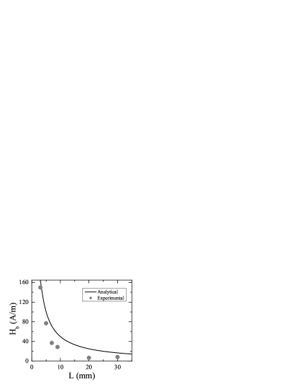
Figure 6: Bias field as a function of the length of the multilayer microwire. The gray dots correspond to the data measured experimentally and the solid line, the values calculated analytically. Parameters: $t_{e}=11$ $\mu$m, $R_{i}=8.7$ $\mu$m and $t_{s}=12.1$ $\mu$m. We have used $M_{e}^{0}=1.2\times 10^{6}$ A/m.

V Discussion and Conclusion

The analytical results presented above may be extended to include other parameter variations. Figure 7 illustrates the magnetostatic bias field as a function of $t_{e}$ for different values of (a) $R_{i}$, (b) $L$ and (c) the width of the spacer, $t_{s}$. In the range of parameters considered, we observe that an increase in $R_{i}$ results in an increase of the magnetostatic bias field. Furthermore, an increase of the length, $L$, produces a decrease of the magnetostatic bias field. Finally, increasing the spacer between the two magnetic layers produces a decrease of the magnetostatic bias field felt by the inner microwire.

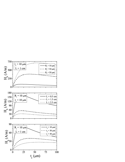
Figure 7: Bias field as a function of $t_{e}$ for different values of (a) $R_{i}$, (b) $L$ and (c) $t_{s}$. We have used $M_{e}^{0}=1.2\times 10^{6}$ A/m.

In summary, we have investigated the magnetostatic biasing effect in multilayer microwires. Using a continuous model we have obtained a simple expression to model the magnetostatic bias in these particles. From our calculations and measurements we can conclude that the magnetostatic bias field strongly depends on the geometry of the system, achieving large values, comparable to the coercivity in some cases. Our results provide guidelines for the production of microstructures with tailored magnetic properties.

VI Acknowledgments

This work was supported by Fondecyt (No. 11070010 and 1080300), Millennium Science Nucleus Basic and Applied Magnetism (project P06-022F), and Spanish MICINN under research project MAT2007-65420-C02-01. M. Bahiana acknowledges support from Instituto do Milenio de Nanotechnologia, MCT/CNPq, FAPERJ, and PROSUL/CNPq.

References

- (1) M. Vazquez, Advanced Magnetic Microwires, in: H. Kronmuller, S. Parkin (Eds.), Handbook of Magnetism and Advanced Magnetic Materials, Wiley, Chichester, UK, 2007, pp. 2193-2296.
- (2) H. Chiriac, M. Tibu, V. Dobrea, and I. Murgulescu, J. Optoelectron. Adv. Mater. 6, 647 (2004).
- (3) K. Mohri, and Y. Honkura, Sensor Lett. 5, 267 (2007).
- (4) E. Kaniusas, L. Mehnen, and H. Pfutzner, J. Magn. Magn. Mater. 254-255, 624 (2003).
- (5) K. Yamada, s. Kasai, Y. Nakatani, K. Kobayashi, H. Kohno, A. Thiaville, and T. Ono, Nat. Mater. 6, 269 (2007).
- (6) I. Ogasawara and S. Ueno, IEEE Trans. Magn. 31, 1219 (1995).
- (7) A. Zhukov, J. Gonzalez, M. Vazquez, V. Larin, and A. Torcunov, in: Nalwa HS, editor. Encyclopedia of Nanoscience and Nanotecnology,vol. X. Stevenson Ranch, CA: American Scientific Publishers; 2003. p.1.
- (8) R. Varga, K. Garcia and M. Vazquez, Phys. Rev. Lett. 94, 017201 (2005).
- (9) J. Nogues, and I. K. Schuller, J. Magn. Magn. Mater. 192, 203 (1999).
- (10) K. Pirota, M. Hernandez-Velez, D. Navas, A. Zhukov and M. Vazquez, Adv. Funct. Mater. 14, 266-268 (2004).
- (11) V. Skumryev, S. Toyanov, Y. Zhang, G. Hadjipanayis, D. Givord, and J. Nogues, Nat. Mater. 423, 850 (2003).
- (12) M. Vazquez, G. Badini-Confalonieri, L. Kraus, K. R. Pirota, and J. Torrejon, Journal of Non-Crystalline Solids 353, 763-767 (2007).
- (13) J. Torrejon, L. Kraus, K. R. Pirota, G. Badini, and M. Vazquez, J. Appl. Phys. 101, 09N105 (2007).
- (14) J. Torrejon, G. Badini, K. Pirota, and M. Vazquez, Acta Materialia 55, 4271-4276 (2007).
- (15) K. R. Pirota, M. Provencio, K. L. Garcia, R. Escobar-Galindo, P. Mendoza Zelis, M. Hernandez-Velez and M. Vazquez, J. Magn. Magn. Mater. 290-291, 68-73 (2005).
- (16) A. Aharoni, Introduction to the Theory of Ferromagnetism, Clarendon Press, Oxford, 1996.
- (17) J. Escrig, S. Allende, D. Altbir, and M. Bahiana, Appl. Phys. Lett. 93, 023101 (2008).
- (18) J. Torrejon, L. Kraus, G. Badini-Confalonieri, and M. Vazquez, Acta Materialia 56, 292-298 (2008).