Glassy dynamics and hysteresis in a linear system of orientable hard rods

Abstract

We study the dynamics of a one-dimensional fluid of orientable hard rectangles with a non-coarse-grained microscopic mechanism of facilitation. The length occupied by a rectangle depends on its orientation, which is coupled to an external field. The equilibrium properties of our model are essentially those of the Tonks gas, but at high densities, the orientational degrees of freedom become effectively frozen due to jamming. This is a simple analytically tractable model of glassy phase. Under a cyclic variation of the pressure, hysteresis is observed. Following a pressure quench, the orientational persistence exhibits a two-stage decay characteristic of glassy systems.

I Introduction

Almost all liquids, if cooled sufficiently fast, form a glassy structure; much effort has been directed towards understanding this phenomenon. Monte Carlo simulations have shown that systems with purely hard-core interactions can describe qualitatively much of the observed phenomenology of the glass transition, e.g., the very fast rise of relaxation times, and the absence of an associated latent heat. Theoretical analysis of such models is hampered by an incomplete understanding of the equilibrium (fluid-solid) phase transition. The best studied hard-core model is a system of hard spheres, which has experimental realizations in colloidal, granular and other systems Pusey and van Megen (1986); Aranson and Tsimring (2006); Prasad et al. (2007). In many cases size dispersion, or other built-in complexity, is introduced in order to avoid crystallization and thereby observe a glass transition Santen and Krauth (2000); Parisi and Zamponi (2005, 2006); Zamponi (2007). For monodisperse systems, there is no transition in one dimension Tonks (1936), while two and three dimensional systems are highly prone to crystallize. In higher dimensions Skoge et al. (2006); van Meel et al. (2009); Zaccarelli et al. (2009); Charbonneau et al. (2010), nucleation rates are low and the glass state is more easily attained. Indeed, in the limit of very high spatial dimensionality, there seems to be an ideal glass transition Parisi and Zamponi (2006); Schmid and Schilling (2010), although how far this extends down to lower dimensions is still debated Tarzia (2007).

Hard core potentials need not be spherically symmetric. On a lattice, for example, where the symmetry is discrete, the behavior strongly depends on the dimension of the system, the lattice structure, and the exclusion range (see Panagiotopoulos (2005); Fernandes et al. (2007a) and refs. therein).

Here we study the dynamic properties of a one-dimensional system of classical hard rectangles, with only two orientations allowed, horizontal and vertical. These will be called “rods” in what follows. Classical linear fluids have been extensively studied over the last decades Tonks (1936); Gürsey (1950); Baxter (1965); Lieb and Mattis (1966); Casey and Runnels (1969); Bloomfield (1970); Percus (1976, 1982); Marko (1989); Davis (1990); Dunlop and Huillet (2003); Fernandes et al. (2007b); Trizac and Pagonabarraga (2008); the case of elongated rods with orientational freedom has also been analyzed Casey and Runnels (1969); Freasier and Runnels (1973); Fulińiski and Longa (1979); Ben-Naim and Krapivsky (2006); Kantor and Kardar (2009a, b); Gurin and Varga (2010). While the equilibrium properties of this class of models are well understood, their dynamic properties, in particular those related to the glass transition, have received somewhat limited attention Bowles (2000); Stadler et al. (2002); Stinchcombe and Depken (2002); Bowles and Saika-Voivod (2006); Dhar and Lebowitz (2010). The simple, one-dimensional model considered here, reproduces (at least in part) the glassy phenomenology with an explicit (non-coarse-grained) microscopic mechanism of facilitation. In analogy with closely related models in which the constraints are kinetic instead of geometric Fredrickson and Andersen (1984); Kob and Andersen (1993); Ritort and Sollich (2003), due to a spatial and temporal coarse-graining, here there is no thermodynamic transition and the only nontrivial behavior is kinetic. In the present context this represents an advantage, in that the relaxation is not complicated by critical slowing down or metastability.

At short time scales, the glassy phase can be modelled as a metastable phase, in restricted thermal equilibrium. An exact calculation of the properties of such metastable states, including the equation of state, has been made recently for a toy model Dhar (2002); Dhar and Lebowitz (2010). In these papers, the ergodicity is explicitly broken, and one assumes that in the glassy phase some transition rates are exactly zero. The simple model considered here provides an extension of the treatment in Ref. Dhar and Lebowitz (2010) to include the description of slow evolution of the macroscopic glassy state at longer time scales. In our model, ergodicity is not explicitly broken, and the dynamics is capable of bringing the system to equilibrium, but at high pressures, the relaxation of orientations becomes so slow that these variables are effectively frozen over any reasonable time scale. Under steady increase of pressure, they never fully relax. Macroscopic properties in the frozen regime are found to depend on history, in particular, on the rate at which the pressure is increased.

The structure of the paper is as follows. The next section introduces the model while Sec. III reviews its equilibrium properties. We describe the dynamic behavior in section IV. Sec. V contains some concluding remarks.

II Model

We consider a system of $N$ rigid rods of length $\sigma\geq 1$ and unit width on a line of length $L$. Each rod is described by the variables $(x_{i},S_{i})$, where $x_{i}\in[0,L)$ is the position of the center of mass and $S_{i}$ denotes its orientation ($0$ for horizontal, 1 for vertical). Rods in state $S_{i}=0$ occupy a length $\sigma$ and those in state $S_{i}=1$ occupy a unit length (see Fig. 1). Since the order of the particles cannot change, we take $x_{1}<x_{2}<\ldots<x_{N}$. For convenience, we define $x_{0}\equiv 0$ and $x_{N+1}\equiv L$; there are no orientational degrees of freedom associated with these variables. We define inter-rod distances, $y_{i}=x_{i+1}-x_{i}$, so that $\sum_{i=0}^{N}y_{i}=L$. When all rods are constrained to have the same orientation or, equivalently, $\sigma=1$, the original Tonks gas Tonks (1936) is recovered. Without this restriction, the model is analogous Onsager (1949) to a binary mixture of rods (with conservation of the total particle number, but not the number of each species separately). The particles are subject to an external field $h^{\prime}$, coupled to the orientations $\{S_{i}\}$, so that the potential energy takes the form

$${\cal H}=\sum_{i}\phi_{\scriptstyle\rm hc}(y_{i})+h^{\prime}\sum_{i}S_{i},$$ (1)

where the first term denotes hard core interactions and the sums extend over the $N$ rods; for $h^{\prime}>0$ the horizontal orientation is favored.

The hard-core interaction between the $i$th rod and its right neighbor is

$$\phi_{\scriptstyle\rm hc}(y_{i})=\begin{cases}0,&y_{i}\geq a_{i}\\ \infty,&y_{i}<a_{i},\end{cases}$$

where $a_{i}$ is the minimum distance between the centers of rods $i$ and $i+1$, given by

$$a_{i}=\sigma+\frac{1}{2}(S_{i}+S_{i+1})(1-\sigma).$$ (2)

An important quantity is the mean free volume per particle, $v_{f}=v-\sigma+(\sigma-1)m$, where $v=\rho^{-1}=L/N$ and $m$ is the fraction of rods in the vertical orientation, or “magnetization”.

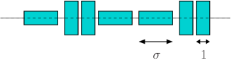
Figure 1: Example of a rod configuration.

We define a local, continuous-time, stochastic dynamics for the positions (or equivalently, the separations $y_{i}$), and orientations. The time evolution is Markovian, and satisfies the detailed balance condition. Each rod executes unbiased diffusive motion. The wall at $x_{N+1}=L$ also undergoes diffusive motion, but is subject to a bias, with ratio of jump rate that increase $L$ by $\delta L$ to the backward transition is $\exp(-p\delta L)$. The rods can also change their orientation, rotating about its center of mass. While the orientation varies continuously during a transition, we suppose the latter occurs so rapidly that orientations other than vertical or horizontal may be neglected. In addition, the dynamics includes an important constraint on orientational transitions: particle $i$ can only change its orientation if its neighbors to the left and right are sufficiently far away that its rotation (through 90^o) is not blocked geometrically (see Fig. 2). In order for particle $i$ to change its orientation, it is necessary that

$$y_{i}>\frac{\sigma+S_{i+1}(1-\sigma)+r}{2}$$ (3)

where $r\equiv\sqrt{1+\sigma^{2}}$ is the rod diagonal. The analogous relation for $y_{i-1}$ must be satisfied as well. Note that these conditions depend on the states of the neighboring rods ($i\pm 1$), but not on $S_{i}$ itself. Without the nonoverlapping constraint, $r$ is replaced by $\sigma$ in the above equation. Any violation of the excluded volume condition is rejected. These transitions are accepted in accordance with the Metropolis criterion, that is, with probability $\min[1,\exp(-\beta\Delta{\cal H})]$. One Monte Carlo step (MCS) consists in an attempt to update all degrees of freedom (i.e., all positions and orientations, and the volume).

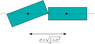
Figure 2: Geometrical constraint associated with an orientational transition. Analogous restrictions apply also for the other possible orientations.

Our Monte Carlo simulations were performed on systems of $N=1000$ rods; and results represent averages over 100 (or more) independent realizations.

III Equilibrium Properties

The equilibrium properties of the model are indeed very simple. The canonical configurational partition function is given by

$$Z_{N}(h,L)=\sum_{\{S_{i}\}}e^{-h\sum_{i}S_{i}}\int_{R}dy_{1}\cdots dy_{N}$$ (4)

where $h=\beta h^{\prime}$ and the subscript $R$ denotes the restrictions $\sum_{i=1}^{N}y_{i}=L$ and $y_{i}\geq a_{i}$, where the minimum distances $a_{i}$ are defined in Eq. (2). The usual factor of $1/N!$ is absent due to the fixed order of the particles on the line. Introducing the variables $z_{i}=y_{i}-a_{i}$, (with $z_{0}\equiv x_{1}$ and $z_{N}\equiv L-x_{N}$), we have,

$$Z_{N}(h,L) = \sum_{\{S_{i}\}}e^{-h\sum_{i}S_{i}}\int_{0}dz_{0}\cdots\int_{0}dz_{N}\;$$

$$\times\delta\left[\sum_{i=0}^{N}z_{i}-L+N\sigma-(\sigma-1)\sum_{i=1}^{N}S_{i}\right].$$

We study the system in the constant-pressure ensemble; the partition function is

$$Y_{N}(h,p)=\int dLe^{-pL}Z_{N}(h,L),$$

where $p$ denotes the pressure divided by $k_{B}T$. A simple calculation yields

$$Y_{N}(h,p)=e^{-pN\sigma}p^{-N}(1+\kappa)^{N}$$ (5)

with $\kappa\equiv\exp[(\sigma-1)p-h]$. The Gibbs free energy per particle is given by $g=-(N\beta)^{-1}\ln Y$, where, in the thermodynamic limit,

$$\lim_{N\to\infty}\frac{1}{N}\ln Y_{N}=-\sigma p+\ln(1+\kappa)-\ln p.$$ (6)

In this limit the volume per particle is,

$$v(p,h)=-\frac{1}{N}\frac{\partial\ln Y}{\partial p}=\sigma-\frac{(\sigma-1)\kappa}{1+\kappa}+\frac{1}{p},$$ (7)

while the fraction of vertical rods is,

$$m_{eq}(p,h)=-\frac{1}{N}\frac{\partial\ln Y}{\partial h}=\frac{\kappa}{1+\kappa}.$$ (8)

Eqs. (7) and (8) imply the relation

$$v=\frac{1}{p}+m_{eq}+\sigma(1-m_{eq}),$$ (9)

which implies that the free volume per particle is $v_{f}=1/p$, as in the Tonks gas. It is worth noting than in equilibrium, the variables $\{y_{i}\}$ and $\{S_{i}\}$ are all mutually independent. The behavior of $m$ as a function of the pressure for several values of $\sigma$ and $h$ is illustrated in Fig. 3.

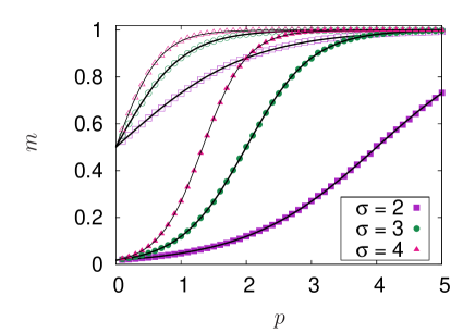
Figure 3: Equilibrium fraction of vertical rods as a function of pressure $p$, for $h=0$ and 4, (empty and filled symbols, respectively). Points are simulation results, while the lines correspond to Eq. (8). When $p$ is large enough, all rods are aligned vertically.

IV Time-dependent Properties

In this section we study the kinetics of the magnetization $m$ and molecular volume $v$. We assume that the diffusive relaxation is much faster than the orientational relaxation. Then the displacement degrees of freedom may be assumed to be in thermal equilibrium. At high pressures, most update attempts for orientation change fail, as they are blocked. Suppose first that the orientations are fixed. In this case, the different sectors in the pico-canonical ensemble are specified by orientation of each rod. Different sectors with the same number of vertical rods are macroscopically equivalent. Within a sector, the displacement degrees of freedom are assumed to be in equilibrium. Then the translational dynamics will bring the system to a constrained equilibrium distribution, in which the distances $z_{i}$ are independent, exponentially distributed random variables with mean $1/p$, and the mean length of the system is $\langle L\rangle=N[1+(1-m)\sigma]+(N+1)/p]$, where $m$ is the fraction of vertically oriented particles, not necessarily equal to the equilibrium value $m_{eq}$.

Now, allowing the orientations to fluctuate, an equation of motion for $m(t)$ can be derived if we assume that the translation dynamics is rapid, so that between any pair of successive orientational transitions, the interparticle distances attain the constrained equilibrium distribution mentioned above. Under this hypothesis, the particle orientations are mutually independent, as in equilibrium (we assume as well that the orientations are initially uncorrelated).

Consider, for example, a transition from $S_{i}=0$ to 1. This would be allowed only if the two gaps on the two sides of the rod are large enough. In the restricted equilibrium ensemble, separations are independent, exponentially distributed random variables, $P(y)=p\exp(-py)$, and the probability that a hole larger than $w=(r-\sigma)/2$ appears at one of its sides is $P(v_{f}>w)=\exp[-p(r-\sigma)/2]$. Given that such gaps must exist at both sides and that this flip is against the field, we see that the effective transition rate is proportional to $\exp[-p(r-\sigma)-h]$, and that it is independent of the state of the neighboring rods. Thus we may write the transition rate for $S_{i}=0$ to 1 as

$$\gamma_{+}=\gamma\exp[-p(r-\sigma)-h],$$ (10)

where $\gamma$ is an arbitrary attempt rate, independent of $p$ and $h$. On the other hand, if the transition is from 1 to 0, $w=(r-1)/2$ and

$$\gamma_{-}=\gamma\exp[-p(r-1)].$$ (11)

Note that only $\gamma_{+}$ depends on $h$ and that these rates satisfy detailed balance. For small values of the pressure, free space is abundant and the slowest process is a flip against the field, so that the larger time scale involved is given by $\gamma_{+}^{-1}$. On the other hand, when the pressure is large enough, the production of large enough holes is the dominant slow process and the relevant characteristic time now scales as $\gamma_{-}^{-1}$.

The evolution of $m(t)$ is governed by

$$\frac{dm}{dt}=\gamma_{+}(1-m)-\gamma_{-}m\equiv-\Gamma m+\gamma_{+},$$ (12)

where $\Gamma=\gamma_{+}+\gamma_{-}$. If the rates are time independent, then letting $\phi=m-m_{eq}=m-\gamma_{+}/\Gamma$, we have

$$\frac{d\phi}{dt}=-\Gamma\phi,$$ (13)

showing an exponential approach to equilibrium.

The system is driven out of equilibrium if the pressure (or the external field, $h$) is time-dependent. Suppose that $\gamma_{+}$ and $\gamma_{-}$ depend on time through the pressure. Then we have

$$m(t)=e^{-{\cal G}(t)}\left(m_{0}+\int_{0}^{t}ds\;\gamma_{+}(s)\;e^{{\cal G}(s)}\right),$$ (14)

where

$${\cal G}(t)=\int_{0}^{t}dt^{\prime}\,\Gamma(t^{\prime}).$$ (15)

A particularly interesting example is that of a system initially in equilibrium at pressure $p_{0}$, and subject to a pressure that increases linearly with time, $p(t)=p_{0}+\lambda t$ for $t>0$, where $\lambda$ is the annealing rate. In this case,

$${\cal G}(t)=\frac{\gamma}{\lambda} \left[e^{-h-p_{0}(r-\sigma)}\frac{1-e^{-\lambda(r-\sigma)t}}{r-\sigma}\right.$$

$$\left.+e^{-p_{0}(r-1)}\frac{1-e^{-\lambda(r-1)t}}{r-1}\right]$$ (16)

so that

$$\lim_{t\to\infty}{\cal G}(t)=\frac{\gamma}{\lambda}\left[\frac{e^{-h-p_{0}(r-\sigma)}}{r-\sigma}+\frac{e^{-p_{0}(r-1)}}{r-1}\right],$$ (17)

which is finite for $\lambda>0$. Inserting this result in Eq. (14), we see that the initial magnetization $m_{0}$ is not “forgotten” even when $t\to\infty$. It is easily verified that memory of the initial magnetization persists for a pressure increase of the form $p(t)=p_{0}+\lambda t^{\alpha}$, for any positive values of $\lambda$ and $\alpha$.

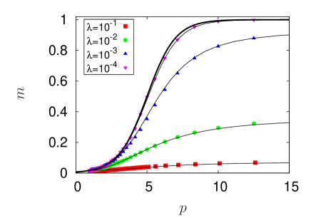
Figure 4: Fraction $m$ of vertical rods versus pressure $p$ for $h=5$, $\sigma=2$, $\gamma=1$ and several values of the rate of pressure increase, $\lambda$. From top to bottom, $\lambda=0$ (equilibrium, bold line), $10^{-3}$, $10^{-2}$, and $10^{-1}$. Points: simulation; solid lines: theory, Eq. (14).

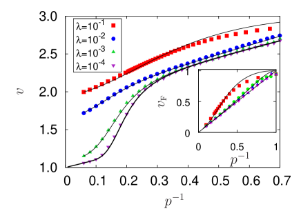
Figure 5: Volume per molecule $v$ versus pressure $p$ for the same parameters as in Fig. 4 during the pressure annealing. Points represent the simulation data while the solid lines are the improved theoretic predictions based on Eq. (18) (with $\gamma\simeq 0.3$). The lines for $\lambda=10^{-4}$ and $\lambda=0$ (equilibrium, bold line) are indistinguishable at this scale. Inset: free volume $v_{F}$. Analogous deviations from equilibrium are again seen for large values of $\lambda$.

Examples of $m(t)$ (for pressure increasing linearly with time) are shown in Fig. 4 for $p_{0}=1$, $h=5$, $\sigma=2$, and $\gamma=1$. For $\lambda=10^{-4}$, the difference between $m(p)$ and the equilibrium result is small. For larger rates of pressure increase, on the other hand, there are marked differences between the final value of $m$ and the equilibrium result. Although $m(t)$ is well described by Eq. (14), as can be seen by the excellent agreement with the simulation, the same does not occur for the molecular volume, $v(p)$, and the free volume, at larger rates of pressure increase $\lambda$. The reason is that in this case the rate of pressure increase is large enough so that we can no longer treat the interparticle distances as in instantaneous thermal equilibrium, on the time scale of the orientational relaxation. This effect can be incorporated in an approximate manner in the theory if we assume that the free volume per molecule follows a relaxational dynamics, that is,

$$\frac{dv_{F}}{dt}=-\Gamma_{v}\left(v_{F}-\frac{1}{p}\right)$$ (18)

To evaluate the transition rates $\gamma_{+}$ and $\gamma_{-}$ we require the probability density $p(z)$. The simplest hypothesis is that $p(z)$ is exponential, as in equilibrium, but with the mean free volume $v_{F}$ in place of its equilibrium value, $1/p$, so that $p(z)=v_{F}^{-1}\exp(-z/v_{F})$. Then the evolution of the magnetization is given by Eq. (12), with transition rates as in Eqs. (10) and (11), but with $p$ replaced by $1/v_{F}$. With an appropriate choice of the relaxation rate $\Gamma_{v}$, this simple theory yields reasonable agreement with simulation results at larger quench rates, as is shown in Fig. 5. Some deviations between the theoretical prediction and simulations are evident at the highest quench rate, for smaller pressures; this is not surprising given the simplifications introduced.

In addition to the “freezing out” of the orientational degrees of freedom under a steady pressure quench, the system exhibits interesting hysteresis effects under an oscillatory pressure. Hysteresis loops obtained through numerical simulation are illustrated in Fig. 6, for various values of $\lambda=|dp/dt|$ in triangle-wave cycles of pressure variation. Similar results are obtained via numerical integration of Eq. (12), assuming rapid equilibration of the free volume. Notice that for larger rates, the system describes a sequence of irreversible loops before entering a reversible one. For even larger rates than those shown in the figure, we find a greater number of irreversible loops, analogous to those obtained in compaction experiments of rods under vibration Villarruel et al. (2000).

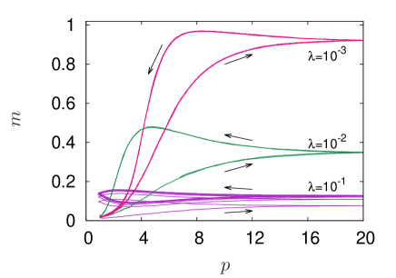
Figure 6: Fraction of vertical rods under cyclic variation of the pressure, showing hysteresis loops. For the highest rate, $\lambda=0.1$, the loop only closes after several cycles. Parameters: $h=5$, $\sigma=2$; the pressure varies between 1 and 20 at rates $\lambda$ as indicated.

It is worth noting that an external field $h$ is not required to observe freezing. Even with $h=0$, the rapid reduction in the transition rate $\gamma_{+}$, Eq. (10), with increasing pressure ensures that the orientational degrees of freedom cannot equilibrate. Inhibition of orientational relaxation is greatest for $\sqrt{1+\sigma^{2}}-\sigma$ as large as possible, i.e., for $\sigma$ tending to unity. (Of course this tends to reduce the excess of $v$ over its equilibrium value.) Thus, for $h=0$, $\sigma=1.1$, and other parameters as above, one finds $m_{\infty}\equiv\lim_{t\to\infty}m(t)=0.620$ if the pressure increases at a rate of $\lambda=1$, and $m_{\infty}=0.5409$ for $\lambda=10$. (As $\lambda$ is increased, $m_{\infty}$ approaches the initial magnetization, equal to $1/2$ for $h=0$.)

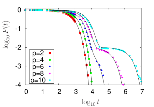
Figure 7: Persistence $P(t)$ as a function of time as the system pressure is quenched from 1 to $p$ at $t=0$, for $\sigma=2$ and $h=5$. When $p$ is small, the decay is exponential while for larger values, after an initial exponential decay, the persistence develops a plateau whose height is close to the initial magnetization $m_{0}$ and whose width increases with $p$. The solid lines are from Eq. (19).

If instead of a smooth annealing, the system is suddenly quenched from low to high pressure, a two-step decay typical of glassy behavior is observed in the orientational persistence (the fraction of rods that did not flip since $t=0$). Fig. 7 shows the results for several values of the final pressure after the system is quenched from an equilibrium state at $p_{0}=1$. Whatever the value of the final pressure, the initial decay of the persistence function is exponential and ruled by the against the field flip of rods that are horizontal at $t=0$, so that $P(t)\simeq\exp(-\gamma_{+}t)$ in this regime. As the final pressure is increased, the flip from 1 to 0 becomes slower and a plateau develops, after the initial fast decay, whose width increases with the final pressure. The height of this plateau is on the order of the initial magnetization, $m_{0}$. (Its precise value is slightly smaller than $m_{0}$ since some of the up rods will have already flipped during the initial fast regime). When the final pressure is large, it takes a long time for a rod to flip, since enough space must be freed, which requires a cooperative rearrangement of the neighboring rods. This happens with a rate proportional to $\gamma_{-}$. Thus, the data in Fig. 7 are well fit by a sum of exponentials, corresponding to the fast and slow processes in the model:

$$P(t)\simeq{\rm e}^{-\gamma_{+}t}+m_{0}{\rm e}^{-b\gamma_{-}t}$$ (19)

where, for the parameters of Fig. 7, $b\simeq 0.4$ and $m_{0}\simeq 0.01$. The coefficient of the second term, 0.01, is the height of the plateau and roughly corresponds to the initial magnetization. Thus, starting with an even smaller initial pressure, and thus a larger magnetization, the plateau can be tuned to higher values. The width of the plateau increases with the final value of the pressure and diverges as $p\to\infty$. This diverging relaxation time, $\gamma_{-}^{-1}$, is related to the increasing length of the cooperative region Kantor and Kardar (2009b). Notice that, at variance with other models for the glass transition, the slow relaxation is not associated with stretched exponentials.

V Conclusions

One-dimensional systems with short-range interactions, such as the model studied here, do not exhibit a phase transition at finite temperature and pressure in equilibrium. A jamming transition involving certain degrees of freedom may nevertheless occur Kantor and Kardar (2009b), with a diverging length scale, as the control parameter (inverse pressure or temperature) goes to zero. Here we study a simple, geometric model on the line, for which analytical results for both the statics and the dynamics may be obtained and compared with numerical simulations, with excellent agreement. This system of hard rods is subject to geometric constraints that prohibit a rod changing its orientation if the distance from its neighbors is too small (i.e., in the absence of sufficient free volume). In our model, the time spent in transit between the two orientations is assumed to be small, and the orientation degree was taken to be a discrete variable. It is straightforward to extend the discussion to the case where we allow continuous orientations, although no qualitative differences are expected.

In the presence of an external field that disfavors the vertical position, our model may be seen as an in-layer description of a higher-dimensional system. In a dense system, the vertical position will be disfavored due to excluded-volume interactions with the rods in the neighboring layers. Thus the external field may be interpreted as an effective interaction to take into account the remaining dimensions.

Despite its simplicity, the model presents several properties characteristic of the glass transition, such as annealing rate dependence and two-step relaxation. The dynamical behavior can be understood in terms of the two microscopic reorientation processes involved.