Spectral representations of vertex transitive graphs, Archimedean solids and finite Coxeter groups

Abstract.

In this article, we study eigenvalue functions of varying transition probability matrices on finite, vertex transitive graphs. We prove that the eigenvalue function of an eigenvalue of fixed higher multiplicity has a critical point if and only if the corresponding spectral representation is equilateral. We also show how the geometric realisation of a finite Coxeter group as a reflection group can be used to obtain an explicit orthogonal system of eigenfunctions. Combining both results, we describe the behaviour of the spectral representations of the second highest eigenvalue function under the change of the transition probabilities in the case of Archimedean solids.

1. Introduction and statement of results

The main objects of interest in this paper are spectral representations associated to random walks on finite graphs (see Sections 1.1 and 1.2 for the definitions). We consider the particular case of vertex transitivity, which comprises the large class of Cayley graphs. In our main result (Theorem 1.3 below), we prove a correspondence between the critical points of an eigenvalue function (under the change of the invariant transition probabilities) and the points where the associated spectral representation is equilateral. In Sections 1.4 and 1.5, we specialise our considerations to finite Coxeter groups and one-skeleta of Archimedean solids.

1.1. Basic graph theoretical notation

Let $G=(V,E)$ be a finite, simple (i.e., no loops and multiple edges) graph with vertex set $V=\{1,\dots,n\}$ and set of undirected edges $E$. An edge is represented by a set $\{i,j\}\subset V$ with $i\neq j$. A (time reversible) random walk on $G$ is given by a symmetric stochastic matrix $P=(p_{ij})\in{{\mathbb{R}}}^{n\times n}$, where $p_{ij}$ is the transition probability from vertex $i$ to vertex $j$. For $i\neq j$, we require $p_{ij}=0$ if $\{i,j\}\not\in E$. Even though there are no loops in $G$, we allow the diagonal elements $p_{ii}$ to be positive. ($p_{ii}$ represents the probability for the random walk to stay at the vertex $i$.) The set of all matrices $P$ of the above type are a convex subset of ${{\mathbb{R}}}^{n\times n}$, which we denote by $\Pi_{G}$. We think of a matrix $P\in\Pi_{G}$ as a linear operator on the vector space $l^{2}(G)$ of (real-valued) functions on the vertices, i.e.,

$$Pf(i)=p_{ii}f(i)+\sum_{j\sim i}p_{ij}f(j),$$

where $j\sim i$ means that $\{i,j\}\in E$. The inner product on $l^{2}(G)$ is given by $\langle f,g\rangle=\sum_{i=1}^{n}f(i)g(i)$. Let $\sigma(P)$ denote the spectrum of $P$ with eigenvalues

$$1=\lambda_{0}(P)\geq\lambda_{1}(P)\geq\cdots\lambda_{n-1}(P)\geq-1,$$

counted with multiplicity. Let $f_{0}(i)=\frac{1}{\sqrt{n}}$. The Rayleigh quotient representation of the second highest eigenvalue function

(1) $$\lambda_{1}(P)=\sup_{f\bot f_{0}\mid f\neq 0}\frac{\langle Pf,f\rangle}{\|f\|^{2}}$$

implies that $\lambda_{1}:\Pi_{G}\to[-1,1]$ is convex (see the proof of Proposition 1.2 in Section 2). The functions $\lambda_{i}:\Pi_{G}\to[-1,1]$ are continuous (see, e.g., [17, Theorem (1,4)]), but these functions fail to be analytic at those points where eigenvalues of higher multiplicity bifurcate. We refer the reader to, e.g., [14, Chapter 2], for more information about these subtle regularity issues. The special operator $P=(p_{ij})$ with vanishing main diagonal ($p_{ii}=0$ for all $i\in V$), and for which all other transition probabilities $p_{ij}$ are equal to $1/{\rm deg}(i)$, is called the canonical Laplacian.

1.2. Spectral representations

The idea of a spectral representation is to use a higher multiplicity eigenvalue of the matrix $P$ to obtain a ”geometric realisation” of the combinatorial graph $G$ in Euclidean space. Assume that $\lambda\in\sigma(P)$ is an eigenvalue of $P$ of multiplicity $k$, and $\phi_{1},\dots,\phi_{k}$ is an orthonormal base of eigenfunctions of the eigenspace ${{{E}}}_{\lambda}(P)$. The corresponding spectral representation is the map

$$\Phi=\Phi_{P,\lambda}:V\to{{\mathbb{R}}}^{k},\quad\Phi(i)=(\phi_{1}(i),\dots,\phi_{k}(i)),$$

i.e., the simultaneous evaluation of all eigenfunctions at a given vertex. The spectral representation depends on the choice of the orthonormal base only up to an orthonormal transformation in ${{\mathbb{R}}}^{k}$.

There are often striking geometric and spectral analogies between the discrete setting of graphs and the smooth setting of Riemannian manifolds. In the context of Riemannian manifolds, the simultaneous evaluation of eigenfunctions of the Laplacian were considered, for example, in the so-called nice (minimal isometric) embeddings of strongly harmonic manifolds into Euclidean spheres (see [5, Chapter 6G]).

Definition 1.1.

A spectral representation $\Phi:V\to{{\mathbb{R}}}^{k}$ is faithful if $\Phi$ is injective. It is equilateral if all images of edges have the same Euclidean length, i.e.,

$$\|\Phi(i_{1})-\Phi(j_{1})\|=\|\Phi(i_{2})-\Phi(j_{2})\|,$$

for all pairs of edges $\{i_{1},j_{1}\},\{i_{2},j_{2}\}\in E$, where $\|\cdot\|$ denotes the Euclidean norm.

A particularly strong faithfulness result for $3$-connected, planar graphs in the case that the second highest eigenvalue has multiplicity three was obtained in [15].

1.3. Vertex transitive graphs

In this paper, we focus on finite vertex transitive graphs, i.e., we assume that the automorphism group ${\rm Aut}(G)$ acts transitively on the vertex set $V$. Particular examples of vertex transitive graphs are Cayley graphs of groups. Below, we introduce equivalence classes of edges and, to have enough flexibility, we consider subgroups $\Gamma\subset{\rm Aut}(G)$ which still act transitively on the vertices. We define a $\Gamma$-action on the space $\Pi_{G}$ of matrices as follows:

$$(\gamma P)_{ij}=p_{\gamma i,\gamma j}\qquad\text{for all $P=(p_{ij})\in\Pi_{G}$.}$$

A random walk and its corresponding matrix $P\in\Pi_{G}$ is called $\Gamma$-invariant, if $\gamma P=P$ for all $\gamma\in\Gamma$. Note that the main diagonal $(p_{11},\dots,p_{nn})$ of every $\Gamma$-invariant matrix $P$ is constant. The large automorphism group of a vertex transitive graph makes the occurence of eigenvalues of higher multiplicities for $\Gamma$-invariant matrices more likely, and it is natural to make use of connections between these eigenvalues and the representation theory of $\Gamma$.

The group $\Gamma$ induces an equivalence relation on the set of edges: $\{i,j\}\in E$ is equivalent to all edges $\{\gamma i,\gamma j\}$ with $\gamma\in\Gamma$. The multiplicity of an equivalence class $[e]\subset E$ is the number of edges in $[e]$ meeting at the same vertex. Let $[e_{1}],\dots,[e_{N}]$ be the $\Gamma$ equivalence classes of edges and $m_{1},\dots,m_{N}$ be its multiplicities. The set of $\Gamma$-invariant matrices in $\Pi_{G}$ with vanishing main diagonal is a convex subset, which we identify with the simplex

(2) $$\Delta_{\Gamma}=\{(x_{1},\dots,x_{N})\in[0,1]^{N}\mid\sum_{j}m_{j}x_{j}=1\}.$$

The point $X=(x_{1},\dots,x_{N})\in\Delta_{\Gamma}$ corresponds to the matrix $P_{X}=(p_{ij})$, given by

$$p_{ij}=\begin{cases}0,&\text{if $i=j$ or $\{i,j\}\not\in E$,}\\ x_{k},&\text{if $\{i,j\}\in[e_{k}]$.}\end{cases}$$

For $P=(p_{ij})\in\Pi_{G}$, let $G_{P}=(V,E_{P})$ denote the subgraph of $G$ with edges $E_{P}=\{\{i,j\}\in E\mid p_{ij}>0\}$. Then, for every interior point $X\in{\rm int}(\Delta_{\Gamma})$, we have $G_{P_{X}}=G$ (since the entries $p_{ij}$ associated to all edges $\{i,j\}$ are strictly positive), and the spectrum $\sigma(P_{X})$ is symmetric with respect to the origin if and only if $G_{P_{X}}$ is bipartite.

Let us now discuss the special case of Cayley graphs. A finite symmetric set $S\subset\Gamma$ of generators of a group $\Gamma$ is called minimal if for every $s\in S$, $S-\{s,s^{-1}\}$ is no longer a set of generators. The Cayley graph of $\Gamma$ with respect to $S$ is denoted by ${\rm Cay}(\Gamma,S)$, its vertices are the group elements, i.e., $V=\Gamma$, and two vertices $\gamma,\gamma^{\prime}$ are connected by an edge if and only if $\gamma^{\prime}=\gamma s$ for some $s\in S$. If $S=\{s_{1},\dots,s_{r}\}$ is a minimal symmetric set of generators, we distinguish the generators of order $2$ (since they appear only once in $S$) from the ones with higher order, by rewriting them as

(3) $$S=\{s_{1},\dots,s_{\nu},\tau_{1}^{\pm 1},\dots,\tau_{\mu}^{\pm 1}\},$$

with $\nu+2\mu=r$. Note that the edges $\{e,\tau_{j}\}$ and $\{e,\tau_{j}^{-1}\}$ are equivalent, and the corresponding simplex $\Delta_{\Gamma}$ is given by

(4) $$\Delta_{\Gamma}=\{(x_{1},\dots,x_{\nu+\mu})\in[0,1]^{N}\mid\sum_{j=1}^{\nu}x_{j}+2\sum_{j=1}^{\mu}x_{\nu+j}=1\}.$$

The following facts follow from the convexity of $\lambda_{1}:\Pi_{G}\to[-1,1]$ (see Section 2 for the proof).

Proposition 1.2.

Let $G=(V,E)$ be a finite, connected, simple graph and $\Gamma\subset{\rm Aut}(G)$ be vertex transitive. Then a global minimum of $\lambda_{1}:\Pi_{G}\to[-1,1]$ is assumed at a matrix in $\Delta_{\Gamma}$.

If $G={\rm Cay}(\Gamma,S)$ is the Cayley graph of a finite group $\Gamma$ with respect to a minimal symmetric set $S$ of generators, then we have

(5) $$\lim_{n\to\infty}\lambda_{1}(P_{X_{n}})=1$$

for every sequence $X_{n}\to\partial\Delta_{\Gamma}$, and a global minimum of $\lambda_{1}$ is assumed at an interior point of $\Delta_{\Gamma}$.

Note that the above result does not rule out that $\lambda_{1}$ may also have other global minima at matrices $P\in\Pi_{G}-\Delta_{\Gamma}$.

Our main general result is the following relation between critical points of eigenvalue functions and equilateral spectral representations:

Theorem 1.3.

Let $G=(V,E)$ be a finite, connected, simple graph and $\Gamma\subset{\rm Aut}(G)$ be vertex transitive. Let $U\subset\Delta_{\Gamma}$ be an open set and $\lambda:U\to[-1,1]$ be a smooth function such that $\lambda(X):=\lambda(P_{X})$ is an eigenvalue of $P_{X}$ with fixed multiplicity $k\geq 2$ for all $X\in U$. $X_{0}\in U$ is a critical point of the function $\lambda$ if and only if the spectral representation $\Phi=\Phi_{P_{X_{0}},\lambda(X_{0})}:V\to S^{k-1}$ is equilateral.

It is shown in Lemma 2.1 (see Section 2) that, for vertex transitive graphs, the image of every $\Gamma$-invariant spectral representation $\Phi=\Phi_{P_{X},\lambda}$ (with $\lambda\in\sigma(P_{X})$ of multiplicity $k$) lies on an Euclidean sphere $S^{k-1}\subset{{\mathbb{R}}}^{k}$, and that equivalent edges are mapped to segments with the same Euclidean length, i.e., $\|\Phi(\gamma i)-\Phi(\gamma j)\|=\|\Phi(i)-\Phi(j)\|$. The above theorem states that at critical points of the eigenvalue function all Euclidean images of edges have the same length (not only the equivalent ones).

Remarks 1.4.

(a) Special examples of critical points are minima of a smooth function. As another example for similarities between graphs and Riemannian manifolds, we like to mention the following result in Riemannian geometry: The first non-zero Laplace-eigenvalue $\lambda_{1}(M)>0$ of a closed Riemannian manifold $(M,g)$ of dimension $n$ with lower positive Ricci curvature is minimal if and only if $M$ is isometric to the $n$-dimensional round sphere (Obata’s theorem, see [18] or [4]). Here we also have the phenomenon that a critical point of the eigenvalue function is assumed in the case of a very symmetric geometry.

(b) For extremal eigenvalues of the Laplace matrix of general graphs, related embedding interpretations arose, e.g., in [12, 11] in studying the semidefinite duals of associated eigenvalue optimization problems. The relation of these results to the vertex symmetric graphs studied here becomes more apparent when symmetry is exploited in the corresponding optimization problems by the techniques described, e.g., in [10, 3]. The precise nature of this relation, however, still needs to be explored further.

Standard arguments in representation theory yield the following useful result:

Proposition 1.5.

Let $\Gamma$ be a finite group with a minimal symmetric set of generators $S$ given by (3) and $G={\rm Cay}(\Gamma,S)$ be the associated Cayley graph with the corresponding simplex $\Delta_{\Gamma}$ as in (4).

Let $\rho:\Gamma\to O(k)$ be an irreducible representation, $\pi_{r}:{{\mathbb{R}}}^{k}\to{{\mathbb{R}}}$ be the projection to the $r$-th coordinate and $S^{k-1}\subset{{\mathbb{R}}}^{k}$ be the unit sphere. Let $p\in S^{k-1}$, $\lambda\in{{\mathbb{R}}}$, and $X=(x_{1},\dots,x_{\nu+\mu})\in\Delta_{\Gamma}$ such that

(6) $$\lambda p=\sum_{j=1}^{\nu}x_{j}\rho(s_{j})p+\sum_{j=1}^{\mu}x_{\nu+j}(\rho(\tau_{j})p+\rho(\tau_{j}^{-1})p).$$

Then the functions

$$\phi_{r}:\Gamma\to{{\mathbb{R}}},\quad\phi_{r}(\gamma):=\pi_{r}(\rho(\gamma)p),\quad 1\leq r\leq k$$

are pairwise orthogonal eigenfunctions of $P_{X}$ for the eigenvalue $\lambda$ satisfying $\|\phi_{r}\|^{2}=\frac{|\Gamma|}{k}$.

Remarks 1.6.

(a) This result implies that if the eigenspace ${{{E}}}_{\lambda}(P_{X})$ is an irreducible representation of $\Gamma$ (i.e., $\phi_{1},\dots,\phi_{k}$ span the whole eigenspace ${{{E}}}_{\lambda}(P_{X})$), then the associated spectral representation $\Phi:\Gamma\to S^{k-1}$ coincides with the orbit map $\Phi(\gamma)=\rho(\gamma)p_{0}$ of the rescaled point $p_{0}=\sqrt{\frac{k}{|\Gamma|}}\,p\in{{\mathbb{R}}}^{k}$. Thus a natural question is whether eigenspace representations are irreducible, or whether different representations appear with the same eigenvalue.

(b) It can be shown, in the weaker case of a non-orthogonal irreducible representation $\rho:\Gamma\to GL(k,{{\mathbb{R}}})$, that the functions $\phi_{r}$ are still a family of linear independent eigenfunctions of $P_{X}$.

1.4. Finite irreducible Coxeter groups

Let us now consider the special case of a finite irreducible Coxeter group $\Gamma=\langle S=\{s_{1},\dots,s_{k}\}\mid(s_{i}s_{j})^{m_{ij}}=e\rangle$ of rank ${\rm rk}(\Gamma)=k$ with $m_{ij}=m_{ji}\geq 2$ and $m_{ii}=2$, i.e., $s_{i}^{2}=e$. It was suggested in [16, Problem 10.8.7] to study the eigenvalues (or at least $\lambda_{1}$) of the canonical Laplacian for Coxeter groups. Bacher [2] identified $\lambda_{1}$ of the canonical Laplacian for symmetric groups. For the canonical Laplacian on arbitrary finite Coxeter groups, Akhiezer [1] found an explicit set of eigenvalues and a lower bound on their multiplicity in case of irreducibility. The spectral gap of the canonical Laplacian and the Kazdhan constant of all finite Coxeter groups was explicitly derived by Kassabov in [13, Section 6.1]. For infinite Coxeter groups, it was proved in [6] that they do not have Kazdhan property $(T)$. In this section we are concerned with Laplacians on finite, irreducible Coxeter groups with variable weights.

Let $\Gamma\hookrightarrow O(k)$ be the geometric realisation of $\Gamma$ as finite reflection group. The associated Cayley graph $G={\rm Cay}(\Gamma,S)$ is bipartite, since all relations of a Coxeter group have even length. Let $\sigma_{j}\in O(k)$ be the reflections corresponding to the generators $s_{j}$ and $n_{1},\dots,n_{k}$ be the associated simple roots. Let

(7) $$p_{j}=(-1)^{j-1}n_{1}\times\cdots\times\mathaccent 866{n_{j}}\times\cdots\times n_{k},$$

where $v_{1}\times\cdots\times v_{k-1}$ denotes the $(k-1)$-ary analogue of the cross product in ${{\mathbb{R}}}^{k}$, and the hat over $n_{j}$ in (7) means that this term is dropped. Then the open cone

$${{\mathcal{F}}}:=\{\alpha_{1}p_{1}+\cdots+\alpha_{k}p_{k}\mid\alpha_{1},\dots,\alpha_{k}>0\}\subset{{\mathbb{R}}}^{k},$$

is a fundamental domain of the $\Gamma$-action on ${{\mathbb{R}}}^{k}$. $\Gamma$ preserves the unit sphere $S^{k-1}$, and a spherical fundamental domain is given by ${{\mathcal{F}}}_{0}={{\mathcal{F}}}\cap S^{k-1}$. Let $V=\det(n_{1},\dots,n_{k})$. Without loss of generality, we can assume that $V>0$, for otherwise we simply permute the set of generators. The following result is a consequence of Proposition 1.5.

Corollary 1.7.

Let $\Gamma$ be a finite, irreducible Coxeter group and ${{\mathcal{F}}}_{0}\subset S^{k-1}$ and $\Delta=\Delta_{\Gamma}$ be as above. Then there exists smooth maps $\Psi_{\Delta}:{{\mathcal{F}}}_{0}\to{\rm int}(\Delta)$ and $\Psi_{\lambda}:{{\mathcal{F}}}_{0}\to(0,1)$, with $\Psi_{\Delta}$ bijective, such that, for every $p=\sum\alpha_{j}p_{j}\in{{\mathcal{F}}}_{0}$, the functions $\phi_{i}(\gamma):=\pi_{i}(\gamma p)$ are pairwise orthogonal eigenfunctions of $P_{X}$ on ${\rm Cay}(\Gamma,S)$ for the eigenvalue $\lambda=\Psi_{\lambda}(p)$, where $X=\Psi_{\Delta}(p)$. Moreover, $\|\phi_{i}\|^{2}=\frac{|\Gamma|}{k}$ and the composition $\Psi_{\lambda}\circ\Psi_{\Delta}^{-1}:{\rm int}(\Delta)\to(0,1)$ is analytic. The simultaneous evaluation

$$\Phi(\gamma):\Gamma\to S^{k-1},\quad\Phi(\gamma)=(\phi_{1}(\gamma),\dots,\phi_{k}(\gamma))=\gamma p$$

is faithful, and the Euclidean lengths of the images of equivalence classes of edges under $\Phi$ are given by

$$\|p-\sigma_{j}(p)\|=2\alpha_{j}V.$$

Remark 1.8.

The explicit description of the maps $\Psi_{\Delta}$, $\Psi_{\lambda}$ and the composition $\Psi_{\lambda}\circ\Psi_{\Delta}^{-1}$ is given by the equations (16), (17), (18) and (20) in Section 3.

The next result follows from a slight modification of a calculation given in Kassabov [13].

Proposition 1.9.

Let $\Gamma,\Psi_{\Delta}$ and $\Psi_{\lambda}$ be as in Corollary 1.7. Then the map $\Psi_{\lambda}\circ\Psi_{\Delta}^{-1}:{\rm int}(\Delta)\to(0,1)$ coincides with the second highest eigenvalue function $\lambda_{1}:{\rm int}(\Delta)\to(0,1)$. Consequently, the second highest eigenvalue $\lambda_{1}(X)$ of $P_{X}$ has always multiplicity $\geq{\rm rk}(\Gamma)$.

The proof of the next result on the exact multiplicity of the second highest eigenvalue for particular Coxeter groups is based on elegant arguments of van der Holst [20]. He used these arguments to give a direct combinatorial proof of Colin de Verdierè’s planarity characterisation ”$\mu(G)\leq 3$”.

Proposition 1.10.

Let $\Gamma$ be one of the Coxeter groups $A_{3}$, $B_{3}$ or $H_{3}$. Then the second highest eigenvalue $\lambda_{1}(X)$ of $P_{X}$ has multiplicity equals three for all $X\in{\rm int}(\Delta)$.

Remark 1.11.

(a) The heart of the proof of Proposition 1.10, namely van der Holst’s argument, is geometric and depends on the planarity of the associated Cayley graphs. It is likely that for every finite, irreducible Coxeter group $\Gamma$ (not only $A_{3},B_{3},H_{3}$) the multiplicity of the second highest eigenvalue function is constant and equal to the rank of $\Gamma$. The techniques in Kassabov’s paper [13] might be useful to prove this general statement.

(b) The value of $\lambda_{1}(X)$ has a well known dynamical interpretation: Our Cayley graphs are bipartite, i.e., we have a partition $V=V_{0}\cup V_{1}$. $\lambda_{1}(X)$ measures the convergence rate of the corresponding random walk to the equidistribution (mixing rate) on each set of vertices $V_{i}$ under even time steps (even time steps are needed because of the bipartiteness). The validity of the multiplicity assumption in (a) together with our main result (Theorem 1.3) would allow us to explicitly determine, for all finite, irreducible Coxeter groups, the transition probabilities of a random walk with the fastest mixing rate on the corresponding Cayley graphs. In fact, this is precisely how we will prove Theorem 1.12 below.

1.5. Archimedean solids

The Cayley graph of the Coxeter groups $A_{3},B_{3}$ and $H_{3}$ (with respect to their set of standard generators $\{s_{1},s_{2},s_{3}\}$) conincide, combinatorially, with the one-skeleta of the Archimedean solids with the vertex configurations $(4,6,6),(4,6,8)$, and $(4,6,10)$, respectively.

Archimedean solids are polyhedra in ${{\mathbb{R}}}^{3}$ such that all faces are regular polygons, and which have a symmetry group acting transitively on the vertices. (Note, however, that the prisms, antiprisms and Platonic solids, which also have these properties, are excluded). The $13$ Archimedean solids are classified via their vertex configurations: The vertex configuration $(m,n,k)$ stands for the solid where an $m$-gon, an $n$-gon and a $k$-gon (in this order) meet at every vertex. We will use this notation also for Platonic solids (e.g., the icosahedron is denoted by $(3,3,3,3,3)$). The spectra of the canonical Laplacians (on the one-skeleta) of all Archimedean solids were explicitly calculated in [19]. For all these graphs, the second highest eigenvalue of the canonical Laplacian has multiplicity three. The corresponding spectral representation is faithful and represents a polyhedron in ${{\mathbb{R}}}^{3}$ (this follows, e.g., from the general result in [15]), but this polyhedron is generally not equilateral. It is natural to study the deformation of this polyhedron under changes of the $\Gamma$-invariant transition probabilities (assuming that the multiplicity of $\lambda_{1}$ does not change), and to find points at which the spectral representation is equilateral.

We will carry this out in the case of the largest Archimedean solid, namely the truncated icosidodecahedron $(4,6,10)$. We will also explain, how the corresponding results read in the case of the Archimedean solids $(4,6,8)$ and $(4,6,6)$. The proofs for these cases are completely analogous.

Let $G=(V,E)$ be the one-skeleton of the Archimedean solid $(4,6,10)$. The automorphism group of $G$ is the full icosahedral group and acts simply transitively on the vertex set $V$, and is isomorphic to $H_{3}$. Considering $G$ as a planar graph, its faces are $4$-, $6$- and $10$-gons. $G$ is $3$-connected, has $120$ vertices and every vertex has degree three (see Figure 1 below). Let $\varphi=\frac{1+\sqrt{5}}{2}=2\cos\frac{\pi}{5}$ be the golden ratio. Our previous results imply the following facts for $\lambda_{1}$.

Theorem 1.12.

Let $G$ be the $1$-skeleton of the Archimedean solid $(4,6,10)$ and $\Gamma={\rm Aut}(G)$. The simplex of $\Gamma$-invariant transition probabilities is

$$\Delta=\Delta_{\Gamma}=\{(x,y,z)\mid x,y,z\geq 0,x+y+z=1\},$$

where $x,y,z$ are the transition probabilities for the edge-equivalence classes separating $4$- and $6$-gons, $4$- and $10$-gons, and $6$- and $10$-gons, respectively. Then the restriction of $\lambda_{1}:\Pi_{G}\to[-1,1]$ to ${\rm int}(\Delta)\subset\Pi_{G}$ is analytic and strictly convex, and $\lambda_{1}(X)$ has multiplicity three for all $X\in{\rm int}(\Delta)$. Moreover, $X_{0}=\frac{1}{14+5\varphi}(5,3+3\varphi,6+2\varphi)$ is the unique point in $\Delta$ at which $\lambda_{1}$ assumes its global minimum with

$$\lambda_{1}(X_{0})=\frac{10+7\varphi}{14+5\varphi}.$$

The corresponding spectral representation $\Phi_{X_{0}}:V\to S^{2}$ is faithful and equilateral.

Let us stress, again, that for $X_{*}=(1/3,1/3,1/3)\in\Delta$, the above Theorem implies that the spectral representation of $P_{X_{*}}$ for $\lambda_{1}(X_{*})$ does not reproduce the Archimedean solid, one has to choose the point $X_{0}\in\Delta$ instead (see Figure 1).

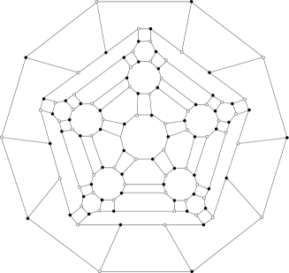
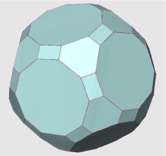
Figure 1. The $1$-skeleton of the Archimedean solid $(4,6,10)$ and the (non-equilateral) spectral representation of the canonical Laplacian for the second highest eigenvalue.

Remark 1.13.

There are analogous versions of Theorem 1.12 in the cases $(4,6,8)$ and $(4,6,6)$. The full symmetry group of both solids $(4,6,8)$ and $(4,6,6)$ is the full octahedral group, but it is better to view $(4,6,6)$ as a polyhedron with the full tetrahedral group (which is a subgroup of the full octahedral group) as its symmetry group, by distinguishing its hexagonal faces with the help of two colours (say, yellow and blue), such that adjacent $6$-gons have different colours. In this case the solid $(4,6,6)$ is also called the omnitruncated tetrahedron and has three equivalence classes of edges (separating $4$-gons and yellow $6$-gons, $4$-gons and blue $6$-gons, yellow and blue $6$-gons), just as the solid $(4,6,8)$ and $(4,6,10)$. The corresponding explicit values for $X_{0}$ and $\lambda_{1}(X_{0})$ are

$$X_{0}=\frac{1}{13+6\sqrt{2}}(4+\sqrt{2},3+3\sqrt{2},6+2\sqrt{2})\quad\text{and}\ \lambda_{1}(X_{0})=\frac{11+6\sqrt{2}}{13+6\sqrt{2}}$$

in the case $(4,6,8)$ and

$$X_{0}=(\frac{3}{10},\frac{3}{10},\frac{2}{5})\quad\text{and}\ \lambda_{1}(X_{0})=\frac{4}{5}$$

in the case $(4,6,6)$.

Finally, we describe the behaviour of spectral representations $\Phi_{X}:V\to S^{2}$, as $X\in\Delta$ moves towards the boundary $\partial\Delta$.

Theorem 1.14.

Let $G,\Delta,X_{0}$ be as in Theorem 1.12. Then there are three explicitly given curves $C_{1},C_{2},C_{3}\subset\Delta$, which meet in $X_{0}$ and have the following property: For every $X\in C_{i}$, the lengths of two of the three equivalence classes of Euclidean edges in the spectral representation of $P_{X}$ for the eigenvalue $\lambda_{1}(X)$ coincide.

As $X_{n}$ converges to the corresponding vertex of the simplex $\Delta$ along the curve $C_{i}$, the spectral representations converge to equilateral realisations of the Archimedean solids $(3,10,10)$, $(5,6,6)$ and $(3,4,5,4)$, respectively.

For any sequence $X_{n}\in{\rm int}(\Delta)$ converging to an interior point of the boundary edge of the simplex $\Delta$, the spectral representations converge to the equilateral realisations of one of the solids $(3,3,3,3,3)$, $(5,5,5)$ and $(3,5,3,5)$.

These convergence properties are illustrated in Figure 2.

\psfrag{c1}{$C_{1}$}\psfrag{c2}{$C_{2}$}\psfrag{c3}{$C_{3}$}\psfrag{(4,6,10)}{\small$(4,6,10)$}\psfrag{(3,3,3,3,3)}{\small$(3,3,3,3,3)$}\psfrag{(3,5,3,5)}{\small$(3,5,3,5)$}\psfrag{(3,4,5,4)}{\small$(3,4,5,4)$}\psfrag{(3,10,10)}{\small$(3,10,10)$}\psfrag{(5,6,6)}{\small$(5,6,6)$}\psfrag{(5,5,5)}{\small$(5,5,5)$}\psfrag{Simplex}{Simplex $\Delta_{\Gamma}$}\includegraphics[height=113.81102pt]{archconv1.eps}

Figure 2. Convergence behaviour of $\Phi_{X}$ as $X\to\partial\Delta$.

Figure 3 shows the spectral representations of $P_{X}$ for three points $X$ along the curve $C_{2}$, illustrating the transition from the dodecahedron $(5,5,5)$ to the buckeyball $(5,6,6)$.

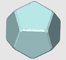
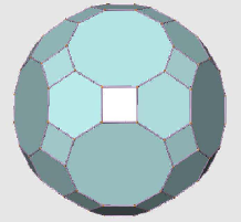
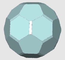
Figure 3. Spectral representations of $P_{X}$ (for points $X$ along $C_{2}$) for the second highest eigenvalue.

Remark 1.15.

The analogous versions of Theorem 1.14 for the Archimedean solids $(4,6,8)$ and $(4,6,6)$ are illustrated in Figure 4 below. The common symmetry group of all solids in the diagram containing $(4,6,8)$ is the full octahedral group. In the diagram containing $(4,6,6)$, we need to colour the hexagons in the solid $(4,6,6)$ with two different colours (as described in Remark 1.13) and, similarly, we have to colour the triangles of the solid $(3,4,3,4)$ with two colours such that triangles meeting in a vertex have different colours (and refer to $(3,4,3,4)$ then as the cantellated tetrahedron), so that the common symmetry group of all solids in this diagram is the full tetrahedral group.

\psfrag{c1}{$C_{1}$}\psfrag{c2}{$C_{2}$}\psfrag{c3}{$C_{3}$}\psfrag{(4,6,8)}{\small$(4,6,8)$}\psfrag{(3,3,3,3)}{\small$(3,3,3,3)$}\psfrag{(3,4,3,4)}{\small$(3,4,3,4)$}\psfrag{(3,4,4,4)}{\small$(3,4,4,4)$}\psfrag{(3,8,8)}{\small$(3,8,8)$}\psfrag{(4,6,6)}{\small$(4,6,6)$}\psfrag{(4,4,4)}{\small$(4,4,4)$}\psfrag{(4,6,6)}{\small$(4,6,6)$}\psfrag{(3,3,3)}{\small$(3,3,3)$}\psfrag{(3,4,3,4)}{\small$(3,4,3,4)$}\psfrag{(3,6,6)}{\small$(3,6,6)$}\psfrag{(4,6,6)}{\small$(4,6,6)$}\includegraphics[height=113.81102pt]{archconv2.eps}

Figure 4. Boundary convergence behaviour in the cases $(4,6,8)$ and $(4,6,6)$.

1.6. Structure of the article

Section 2 provides the proofs of Propositions 1.2 and 1.5 and of our Main Theorem 1.3. In Sections 3 and 4, we prove Corollary 1.7 and Propositions 1.9 and 1.10. Finally, Section 5 presents the proofs of Theorems 1.12 and 1.14.

Acknowlegdements: We are grateful to Stefan Dantchev, Christoph Helmberg, Dirk Schütz and Ivan Veselić for many helpful comments. Moreover, we like to express our gratitude to the referee for providing us with the proof of Proposition 1.9, and for many other useful comments which improved and simplifed parts of our article.

2. Proofs of the general results

Let us start with a convexity proof of $\lambda_{1}:\Pi_{G}\to[-1,1]$, which is used to show that $\lambda_{1}$ assumes a global minimum in $\Delta_{\Gamma}$.

Proof of Proposition 1.2: First note that, for $P,P^{\prime}\in\Pi_{G}$ and $\alpha\in[0,1]$,

$$\frac{\left\langle(\alpha P+(1-\alpha)P^{\prime})f,f\right\rangle}{\|f\|^{2}}=\alpha\frac{\langle Pf,f\rangle}{\|f\|^{2}}+(1-\alpha)\frac{\langle P^{\prime}f,f\rangle}{\|f\|^{2}},$$

which implies the convexity of $\lambda_{1}:\Pi_{G}\to[-1,1]$ by taking supremums on both sides and using the characterisation (1).

Note also that $\Pi_{G}$ is compact, and the continuous function $\lambda_{1}:\Pi_{G}\to[-1,1]$ must have a global minimum at some point $P\in\Pi_{G}$. If $P\not\in\Delta_{\Gamma}$, then consider the $\Gamma$-invariant matrix $P^{\prime}=\frac{1}{|\Gamma|}\sum_{\gamma\in\Gamma}\gamma P\in\Pi_{G}$, and we conclude $\lambda_{1}(P^{\prime})\leq\lambda_{1}(P)$ by the convexity of $\lambda_{1}$. $P^{\prime}$ may have a non-vanishing (constant) main diagonal. Nevertheless, we can write $P^{\prime}=\beta{\rm Id}+(1-\beta)P^{\prime\prime}$ with appropriate $P^{\prime\prime}\in\Delta_{\Gamma}$ and $\beta\geq 0$. This implies that

$$\lambda_{1}(P^{\prime})-\lambda_{1}(P^{\prime\prime})=\beta(1-\lambda_{1}(P^{\prime\prime}))\geq 0,$$

which shows that $\lambda_{1}$ assumes also a global minimum at $P^{\prime\prime}\in\Delta_{\Gamma}$.

Now, assume that $G={\rm Cay}(\Gamma,S)$ and that $S$ is a minimal set of generators. The minimality of $S$ implies that, for every $X\in\partial\Delta_{\Gamma}$, the graph $G_{P_{X}}$ consists of more than one connected component and, therefore, $\lambda_{0}(P_{X})=\lambda_{1}(P_{X})=1$. Then (5) follows from the continuity of the function $\lambda_{1}$. For every interior point $X\in\Delta_{\Gamma}$ we have $\lambda_{1}(P_{X})<1$, since $G_{P_{X}}$ is connected. $\Box$

Our next goal is the proof that $\Gamma$-invariant spectral representations map all vertices onto a sphere and that equivalent edges are mapped to Euclidean segments of the same length.

Lemma 2.1.

Let $G=(V,E)$ be a simple finite graph and $\Gamma\subset{\rm Aut}(G)$ be vertex transitive with $N$ equivalence classes of edges, and $\Delta_{\Gamma}$ be as in (2). Let $X\in\Delta_{\Gamma}$ and $\lambda\in[-,1,1]$ be an eigenvalue of multiplicity $k\geq 2$ of the operator $P_{X}$. Let $\Phi=\Phi_{X,\lambda}:V\to{{\mathbb{R}}}^{k}$ be the associated spectral representation. Then there exist constants $c>0$, $c_{1},\dots,c_{N}\geq 0$ such that

• for all vertices $i\in V$: $\|\Phi(i)\|=c$,

• for all edges $\{i,j\}\in E$ in the $l$-th equivalence class

  $$\|\Phi(i)-\Phi(j)\|=c_{l}.$$

Proof: Let $\phi_{1},\dots,\phi_{k}$ be the orthonormal basis of eigenfunctions defining $\Phi=(\phi_{1},\dots,\phi_{k})^{\top}$ (we consider $\Phi(i)$ as a column vector). Let $\gamma\in\Gamma$ be fixed and $\psi_{r}=\phi_{r}\circ\gamma:V\to{{\mathbb{R}}}$. One easily checks that $\psi_{1},\dots,\psi_{k}$ are also an orthonormal basis satisfying $P_{X}\psi_{r}=\lambda\psi_{r}$. Consequently, there exists a matrix $C=(c_{rs})\in O(k)$ such that $\psi_{r}=\sum_{s=1}^{k}c_{rs}\phi_{s}$. This implies $\Phi(\gamma i)=C\Phi(i)$ and

(8) $$\langle\Phi(\gamma i),\Phi(\gamma j)\rangle=\langle C\Phi(i),C\Phi(j)\rangle=\langle\Phi(i),\Phi(j)\rangle.$$

(8) implies (a) by choosing $i=j$ and using the vertex transitivity of $\Gamma$. (b) follows from (a), (8) and

$$\|\Phi(i)-\Phi(j)\|^{2}=\|\Phi(i)\|^{2}-2\langle\Phi(i),\Phi(j)\rangle+\|\Phi(j)\|^{2}.$$

$\Box$

Before entering into the proof of our main result, let us remark that the above identity (8) can be rewritten as

(9) $$\sum_{r=1}^{k}\phi_{r}(i)\phi_{r}(j)=\sum_{r=1}^{k}\phi_{r}(\gamma i)\phi_{r}(\gamma j)\quad\text{for all $i,j\in V$ and $\gamma\in\Gamma$}.$$

Moreover, observe that the following identity is an immediate consequence of the vertex transitivity of $\Gamma$, the left coset decomposition $\Gamma=\gamma_{1}\Gamma_{1}\cup\gamma_{2}\Gamma_{1}\cup\cdots\cup\gamma_{n}\Gamma_{1}$, where $\Gamma_{1}\subset\Gamma$ is the stabilizer of $1\in V$, and the relation $|\Gamma|=n|\Gamma_{1}|$:

(10) $$\sum_{i=1}^{n}f(i)=\frac{n}{|\Gamma|}\sum_{\gamma\in\Gamma}f(\gamma 1).$$

Proof of Theorem 1.3: For simplicity, we discuss the key arguments for the special choice of the first and second equivalence class of edges. The proof for two arbitrary equivalence classes is completely analogous.

Let $\{1,i_{1}\},\dots,\{1,i_{p}\}$ be all edges adjacent to $1\in V$ in the first equivalence class of edges (note that $p=m_{1}$). Let $\{1,j_{1}\},\dots,\{1,i_{q}\}$ be all edges adjacent to $1\in V$ in the second equivalence class of edges (note that $q=m_{2}$). We conclude from (9) that

(11) $$\sum_{r=1}^{k}\phi_{r}(1)\phi_{r}(i_{1})=\sum_{r=1}^{k}\phi_{r}(1)\phi_{r}(i_{2})=\cdots=\sum_{r=1}^{k}\phi_{r}(1)\phi_{r}(i_{p}),$$

and the same identity holds for the edges in the second equivalence class.

Let $X_{0}\in U$ an arbitary point (not necessarily a critical point of $\lambda_{1}$), $\xi=(\frac{1}{p},-\frac{1}{q},0,\dots,0)\in{{\mathbb{R}}}^{N}$ and $X_{t}:=X_{0}+t\xi\in U$ for $t\in(-\epsilon,\epsilon)$ and $\epsilon>0$ suitably small. For simplicity of notation, we introduce $P(t):=P_{X_{t}}$, $\lambda(t)=\lambda(X_{t})$. Let $\phi_{1},\dots,\phi_{k}$ be an orthonormal basis of the eigenspace ${{{E}}}_{\lambda(0)}(P(0))$. Let ${\rm Pr}_{t}$ denote the orthogonal projection of $l^{2}(G)$ onto the eigenspace ${{{E}}}_{\lambda(t)}(P(t))={\rm ker}(P(t)-\lambda(t))$. Since $P(t)$ and $\lambda(t)$ depend smoothly on $t$, ${\rm Pr}_{t}$ is also smooth in $t$. By making $\epsilon>0$ smaller, if needed, we can assume that ${\rm Pr}_{t}\phi_{1},\dots,{\rm Pr}_{t}\phi_{k}$ is a basis of ${{{E}}}_{\lambda(t)}(P(t))$, for all $t\in(-\epsilon,\epsilon)$. Applying Gram-Schmidt to these vectors, we obtain an orthonormal basis $\phi_{1,t},\dots,\phi_{k,t}$ of the eigenspace ${{{E}}}_{\lambda(t)}(P(t))$, depending smoothly on $t$ and satisfying $\phi_{r}=\phi_{r,0}$. Note that $P^{\prime}(0)=(c_{ij})$ with

$$c_{\gamma 1,\gamma i}=\begin{cases}\frac{1}{p},&\text{if $i\in\{i_{1},\dots,i_{p}\}$},\\ -\frac{1}{q},&\text{if $i\in\{j_{1},\dots,j_{q}\}$},\\ 0,&\text{otherwise},\end{cases}$$

for all $\gamma\in\Gamma$ and $i\in V$.

Let $r\in\{1,\dots,k\}$. By the orthonormality of the functions $\phi_{r}$, we have $\langle\phi_{r},\frac{\partial}{\partial t}\big{|}_{t=0}\phi_{r,t}\rangle=0$. Using this and the symmetry of $P(t)$, we obtain, by differentiating $\lambda(t)=\langle P(t)\phi_{r,t},\phi_{r,t}\rangle$ at $t=0$:

$$\lambda^{\prime}(0)=\langle P^{\prime}(0)\phi_{r},\phi_{r}\rangle = \sum_{i=1}^{n}\phi_{r}(i)\left(\sum_{j=1}^{n}c_{ij}\phi_{r}(j)\right)$$

$$= \frac{n}{|\Gamma|}\sum_{\gamma\in\Gamma}\phi_{r}(\gamma 1)\left(\sum_{j=1}^{n}c_{\gamma 1,\gamma j}\phi_{r}(\gamma j)\right)\qquad\text{using \eqref{eq:fundeq}}$$

$$= \frac{n}{|\Gamma|}\sum_{\gamma\in\Gamma}\phi_{r}(\gamma 1)\left(\frac{1}{p}\sum_{s=1}^{p}\phi_{r}(\gamma i_{s})-\frac{1}{q}\sum_{s=1}^{q}\phi_{r}(\gamma j_{s})\right).$$

On the other hand, we have

$$\langle\Phi(1),\Phi(i_{1})\rangle = \frac{1}{p}\sum_{s=1}^{p}\sum_{r=1}^{k}\phi_{r}(1)\phi_{r}(i_{s})\qquad\text{using \eqref{eq:i1ip}}$$

$$= \sum_{r=1}^{k}\frac{1}{|\Gamma|}\sum_{\gamma\in\Gamma}\phi_{r}(\gamma 1)\frac{1}{p}\sum_{s=1}^{p}\phi_{r}(\gamma i_{s})\qquad\text{using \eqref{eq:gammainv}}.$$

Combining both results, we obtain

$$\langle\Phi(1),\Phi(i_{1})\rangle-\langle\Phi(1),\Phi(j_{1})\rangle=\frac{k}{n}\lambda^{\prime}(0).$$

This implies that we have $\|\Phi(1)-\Phi(i_{1})\|=\|\Phi(1)-\Phi(j_{1})\|$ if and only if $\lambda^{\prime}(0)=0$.

Since the above arguments hold for any choice of equivalence classes of edges, we have $c_{1}=\dots=c_{N}$ in Lemma 2.1 above (i.e., an equilateral spectral representation) if and only if the derivative of $\lambda$ at $X_{0}$ vanishes in all directions of the simplex, i.e., if $X_{0}\in U$ is a critical point of $\lambda$. $\Box$

The proof of Proposition 1.5 is based on the following lemma:

Lemma 2.2.

Let $\Gamma$ be a finite group, $\rho:\Gamma\to O(k)$ be an irreducible representation and, as before, $\langle\cdot,\cdot\rangle$ be the standard inner product in ${{\mathbb{R}}}^{k}$. For any non-zero vector $p\in{{\mathbb{R}}}^{k}$ there is a constant $C_{p}>0$ such that

$$\sum_{\gamma\in\Gamma}\langle\rho(\gamma)p,v\rangle\,\langle\rho(\gamma)p,w\rangle=C_{p}\langle v,w\rangle$$

for all $v,w\in{{\mathbb{R}}}^{k}$.

Proof: The expression

$$\langle v,w\rangle_{p}:=\sum_{\gamma\in\Gamma}\langle\rho(\gamma)p,v\rangle\,\langle\rho(\gamma)p,w\rangle$$

is obviously a symmetric bilinear form. The form is positive definite, since $\langle v,v\rangle_{p}=0$ implies that $v$ is perpendicular (w.r.t. the standard inner product) to ${\rm span}\{\rho(\gamma)p\mid\gamma\in\Gamma\}$. Irreducibility of $\rho$ implies that ${\rm span}\{\rho(\gamma)p\mid\gamma\in\Gamma\}={{\mathbb{R}}}^{k}$, so $v=0$. Therefore, there exists a positive definite symmetric matrix $A$ such that

$$\langle v,w\rangle_{p}=\langle Av,w\rangle.$$

Let $\gamma_{0}\in\Gamma$. Then

$$\langle\rho(\gamma_{0})v,\rho(\gamma_{0})w\rangle_{p}=\sum_{\gamma\in\Gamma}\langle\rho(\gamma_{0}^{-1}\gamma)p,v\rangle\langle\rho(\gamma_{0}^{-1}\gamma)p,w\rangle=\langle v,w\rangle_{p},$$

i.e., $\langle\cdot,\cdot\rangle_{p}$ is $\rho(\Gamma)$-invariant, and we have $A\rho(\gamma)=\rho(\gamma)A$ for all $\gamma\in\Gamma$. Since $\rho$ is irreducible, we conclude from Schur’s lemma that $A$ is of the form $C_{p}\cdot{\rm Id}$ with a constant $C_{p}>0$. This finishes the proof of the lemma. $\Box$

Proof of Proposition 1.5: Note that the vertices of $G={\rm Cay}(\Gamma,S)$ are the group elements, and that

$$P_{X}f(\gamma)=\sum_{j=1}^{\nu}x_{j}f(\gamma s_{j})+\sum_{j=1}^{\mu}x_{\nu+j}(f(\gamma\sigma_{j})+f(\gamma\sigma_{j}^{-1})).$$

This implies that

$$P_{X}\phi_{r}(\gamma) = \sum_{j=1}^{\nu}x_{j}\pi_{r}(\rho(\gamma s_{j})p)+\sum_{j=1}^{\mu}x_{\nu+j}(\pi_{r}(\rho(\gamma\sigma_{j})p)+\pi_{r}(\rho(\gamma\sigma_{j}^{-1})p))$$

$$= \pi_{r}\left(\rho(\gamma)\left(\sum_{j=1}^{\nu}x_{j}\rho(s_{j})p+\sum_{j=1}^{\mu}x_{\nu+j}(\rho(\sigma_{j})p+\rho(\sigma_{j}^{-1})p)\right)\right)$$

$$= \lambda\pi_{r}(\rho(\gamma)p)=\lambda\phi_{r}(\gamma),$$

by using (6). This shows that $\phi_{r}$ is an eigenfunction of $P_{X}$ for the eigenvalue $\lambda$. The orthogonality of the functions $\phi_{r}$ is a straightforward application of Lemma 2.2:

$$\langle\phi_{r},\phi_{s}\rangle=\sum_{\gamma\in\Gamma}\pi_{r}(\rho(\gamma)p)\pi_{s}(\rho(\gamma)p)=\sum_{\gamma\in\Gamma}\langle\rho(\gamma)p,e_{r}\rangle\,\langle\rho(\gamma)p,e_{s}\rangle=C_{P}\langle e_{r},e_{s}\rangle,$$

where $e_{1},\dots,e_{k}$ denotes the standard basis in ${{\mathbb{R}}}^{k}$. Now let $\Gamma=\{\gamma_{1},\dots,\gamma_{n}\}$. Let $A$ be the $(k\times n)$ matrix whose columns are the vectors $\rho(\gamma_{j})p\in S^{k-1}$. Then the rows of $A$ represent the functions $\phi_{r}$, and we have

$$\sum_{r=1}^{k}\|\phi_{r}\|^{2}=\sum_{j=1}^{n}\|\rho(\gamma_{j})p\|^{2}=n=|\Gamma|.$$

This shows that $\|\phi_{r}\|^{2}=\frac{|\Gamma|}{k}$. $\Box$

Remark 2.3.

Assume that $\rho$ in Proposition 1.5 is irreducible but not orthogonal, i.e., $\rho:\Gamma\to GL(k,{{\mathbb{R}}})$. The above proof still shows that the functions $\phi_{r}$ are eigenfunctions. Let $A$ be the $(k\times n)$ matrix as in the proof. Then the irreducibility of $\rho$ implies that the columns span all of ${{\mathbb{R}}}^{k}$, i.e., the rank of $A$ is $k$. But this means that the functions $\phi_{r}$ (the $k$ rows of $A$) must be linearly independent.

3. Proof of Corollary 1.7 and Proposition 1.9

Our first aim is to establish the geometric procedure for obtaining eigenfunctions of $P_{X}$ on the Cayleygraph of a Coxeter group, as well as explicit derivations of the maps $\Psi_{\lambda}$ and $\Psi_{\Delta}$.

Proof of Corollary 1.7: We start with a finite, irreducible Coxeter group. This implies that the geometric realisation $\Gamma\hookrightarrow O(k)$ is an irreducible, faithful representation. Note that we have $\langle n_{i},n_{j}\rangle=-\cos\frac{\pi}{m_{ij}}$, where $m_{ij}$ is the order of the element $s_{i}s_{j}$. Since $\Gamma$ is a finite Coxeter group, $M=(\langle n_{i},n_{j}\rangle)$ is a positive definite, symmetric matrix. Writing $M={\rm Id}-C$ with a symmetric matrix $C<{\rm Id}$ (as quadratic forms) whose entries are all non-negative, we obtain $M^{-1}=\sum_{s=0}^{\infty}C^{s}$. Irreducibility implies that for every position $1\leq i,j\leq k$, there is an $s\geq 0$ such that $(C^{s})_{ij}>0$. This implies that all entries of $M^{-1}$ are strictly positive. Recall that

$$V:=\det(n_{1},\dots,n_{k})=\left(\det M\right)^{1/2}>0.$$

We define, as in (7),

$$p_{j}=(-1)^{j-1}n_{1}\times\cdots\times\mathaccent 866{n_{j}}\times\cdots\times\cdots n_{k}.$$

The vectors $p_{j}$ may all have different Euclidean lengths. We have, by construction $\langle n_{i},p_{j}\rangle=V\delta_{ij}$. Let

$$\Delta=\Delta_{\Gamma}=\{(x_{1},\dots,x_{k})\mid x_{j}\geq 0,\sum_{j}x_{j}=1\}$$

be the simplex associated to the Cayley graph ${\rm Cay}(\Gamma,S)$.

Our aim is to construct the maps $\Psi_{\Delta}:{{\mathcal{F}}}_{0}\to{\rm int}(\Delta)$ and $\Psi_{\lambda}:{{\mathcal{F}}}_{0}\to(0,1)$: Any point $p\in{{\mathcal{F}}}_{0}$ can be expressed uniquely as

$$p=\alpha_{1}p_{1}+\cdots+\alpha_{k}p_{k},$$

with $\alpha_{1},\dots,\alpha_{k}>0$. We will show that there is a unique choice of $X=(x_{1},\dots,x_{k})\in{\rm int}(\Delta)$ and $\lambda\in(0,1)$ such that

(12) $$\lambda p=\sum_{j}x_{j}\sigma_{j}(p).$$

We then define $\Psi_{\Delta}(p)=X$ and $\Psi_{\lambda}(p)=\lambda$. The construction will show that $X$ and $\lambda$ depend smoothly on the coordinates $\alpha_{j}$. Applying Proposition 1.5 yields the results stated in the Corollary. It then only remains to prove that $\Psi_{\Delta}$ is bijective and that the composition $\Psi_{\lambda}\circ\Psi_{\Delta}^{-1}$ is analytic.

Since $\sigma_{j}(p)=p-2\langle p,n_{j}\rangle n_{j}=p-2\alpha_{j}Vn_{j}$, we immediately see that $\|p-\sigma_{j}(p)\|=2\alpha_{j}V$. Moreover, (12) translates into

(13) $$\lambda p=(x_{1}+\cdots+x_{k})p-2V\sum_{j}\alpha_{j}x_{j}n_{j}.$$

This means that we need to find a unique $(x_{1},\dots,x_{n})\in\Delta$ and $\mu\in{{\mathbb{R}}}$ such that

(14) $$\sum_{j}\alpha_{j}x_{j}n_{j}=\mu\sum_{j}\alpha_{j}p_{j},$$

and then set $\lambda=x_{1}+\cdots+x_{k}-2V\mu$. Taking inner products with the simple roots $n_{1},\dots,n_{k}$, and bringing everything in a matrix equation, we end up with the equivalent equation

(15) $$M\begin{pmatrix}\alpha_{1}x_{1}\\ \vdots\\ \alpha_{k}x_{k}\end{pmatrix}=\mu V\begin{pmatrix}\alpha_{1}\\ \vdots\\ \alpha_{k}\end{pmatrix}.$$

Obviously, this equation is homogeneous, i.e., if $(x_{1},\dots,x_{k},\mu)$ is a solution then so is $(cx_{1},\dots,cx_{k},c\mu)$ for any constant $c$. We first seek for the unique solution $(x_{1}^{\prime},\dots,x_{k}^{\prime})$ of (15) for the choice $\mu=1$. $(x_{1}^{\prime},\dots,x_{k}^{\prime})$ will not be a point in $\Delta$, and we obtain the correct solution by way of rescaling. Using the fact that $M^{-1}={\rm Id}+D$, where all diagonal entries of $D$ are non-negative and all off-diagonal are strictly positive, we end up with the inequality

(16) $$\begin{pmatrix}x_{1}^{\prime}\\ \vdots\\ x_{k}^{\prime}\end{pmatrix}=V\begin{pmatrix}\alpha_{1}&&\\ &\ddots&\\ &&\alpha_{k}\end{pmatrix}^{-1}M^{-1}\begin{pmatrix}\alpha_{1}&&\\ &\ddots&\\ &&\alpha_{k}\end{pmatrix}\begin{pmatrix}1\\ \vdots\\ 1\end{pmatrix}>V\begin{pmatrix}1\\ \vdots\\ 1\end{pmatrix}.$$

This shows that any choice $\alpha_{1},\dots,\alpha_{k}>0$ leads to a strictly positive vector $(x_{1}^{\prime},\dots,x_{k}^{\prime})$, and that

(17) $$\lambda^{\prime}:=x_{1}^{\prime}+\ +\cdots+x_{k}^{\prime}-2V>0.$$

For $p=\sum_{j}\alpha_{j}p_{j}\in{{\mathcal{F}}}_{0}$, we first calculate $x_{1}^{\prime},\dots,x_{k}^{\prime},\lambda^{\prime}>0$ via the equations (16) and (17), and then apply the rescaling to obtain

(18) $$\Psi_{\Delta}(p)=\frac{1}{\sum_{j}x_{j}^{\prime}}(x_{1}^{\prime},\dots,x_{k}^{\prime})\in{\rm int}(\Delta),\qquad\Psi_{\lambda}(p)=\frac{\lambda^{\prime}}{\sum_{j}x_{j}^{\prime}}\in(0,1).$$

Next we show that $\Psi_{\Delta}:{{\mathcal{F}}}_{0}\to{\rm int}(\Delta)$ is bijective. Choose $X=(x_{1},\dots,x_{k})\in{\rm int}\Delta$. An equivalent reformulation of (15) is

(19) $$\begin{pmatrix}\alpha_{1}\\ \vdots\\ \alpha_{k}\end{pmatrix}=\mu V{\mathbf{x}}^{-1}M^{-1}\begin{pmatrix}\alpha_{1}\\ \vdots\\ \alpha_{k}\end{pmatrix},$$

where ${\mathbf{x}}={\rm diag}(x_{1},\dots,x_{k})$ denotes the diagonal matrix with the entries $x_{j}$. Note that $V\,{\mathbf{x}}^{-1}M^{-1}$ is a matrix with all its entries strictly positive. Therefore, we can apply Perron-Frobenius theory and conclude that there is a unique Perron-Frobenius eigenvector $(\alpha_{1},\dots,\alpha_{k})$, scaled in such a way that $p=\sum_{j}\alpha_{j}p_{j}\in S^{k-1}$. Since $\alpha_{j}>0$, we conclude that $p\in{{\mathcal{F}}}_{0}$. This shows that every $X\in{\rm int}(\Delta)$ has a unique preimage under $\Psi_{\Delta}$.

Moreover, note that $\mu^{-1}$ is the Perron-Frobenius eigenvalue of the matrix $V{\mathbf{x}}^{-1}M^{-1}$ and that $\lambda=\left(\sum_{j}x_{j}\right)-2V\mu=1-2V\mu$ in (13). This implies that the composition $\Psi_{\lambda}\circ\Psi_{\Delta}^{-1}:{\rm int}(\Delta)\to(0,1)$ is given by

(20) $$\Psi_{\lambda}\circ\Psi_{\Delta}^{-1}(X)=1-2\Lambda_{X},$$

where $\Lambda_{X}$ is the Perron-Frobenius eigenvalue of the positive matrix ${\mathbf{x}}^{-1}M^{-1}$. Since this eigenvalue has always multiplicity one, it depends analytically on the weights $x_{1},\dots,x_{k}$, by the analytic version of the Implicit Function Theorem. This finishes the proof of Corollary 1.7. $\Box$

Next we modify arguments in Kassabov [13, p. 20] to prove Proposition 1.9.

Proof of Proposition 1.9: Let us first recall some of his notation of this source. Let ${\mathcal{H}}=l^{2}(G)$ and $\pi:\Gamma\to U({\mathcal{H}})$ be the right-regular representation $(\pi(\sigma)f)(\gamma)=f(\gamma\sigma)$. Let

$$\Delta_{X}={\rm Id}-P_{X}=\sum_{i=1}^{k}x_{i}({\rm Id}-\pi(s_{i})).$$

Let $V_{i}=\{f\in{\mathcal{H}}\mid f=\pi(s_{i})f\}$. Note that ${\rm Id}-\pi(s_{i})$ is equal to $2{\rm Pr}_{V_{i}^{\bot}}$, i.e., twice the orthogonal projection to the orthogonal complement of the subspace $V_{i}$. This implies that

(21) $$\langle\Delta_{X}f,f\rangle=2\sum_{i}x_{i}d_{V_{i}}(f)^{2},$$

where $d_{V}(f)=\inf_{g\in V}\|f-g\|=\|{\rm Pr}_{V^{\bot}}f\|$. Moreover, we have

$$\bigcap_{i=1}^{k}V_{i}=\{\text{constant functions in $l^{2}(G)$}\}.$$

For $f\in{\mathbb{H}}$, let ${\mathbf{d}}_{f}$ denote the column vector with entries the distances $d_{V_{i}}(f)$. We conclude from [13, Thm. 5.1] that, for any function $f$ orthogonal to the constant functions,

(22) $$\|f\|^{2}\leq{\mathbf{d}}_{f}^{\top}M^{-1}{\mathbf{d}}_{f}=({\mathbf{x}}^{1/2}{\mathbf{d}}_{f})^{\top}{\mathbf{x}}^{-1/2}M^{-1}{\mathbf{x}}^{-1/2}({\mathbf{x}}^{1/2}{\mathbf{d}}_{f})\leq\Lambda_{X}\|{\mathbf{x}}^{1/2}{\mathbf{d}}_{f}\|^{2},$$

where $\Lambda_{X}$ is the the Perron-Frobenius eigenvalue of ${\mathbf{x}}^{-1/2}M^{-1}{\mathbf{x}}^{-1/2}$ (note that this agrees with the Perron-Frobenius eigenvalue of ${\mathbf{x}}^{-1}M^{-1}$). Combining (21) and (22), we conclude that

$$\langle\Delta_{X}f,f\rangle\geq 2\Lambda_{X}\|f\|^{2},$$

i.e., the second highest eigenvalue $\lambda_{1}(X)$ of $P_{X}$ is $\leq 1-2\Lambda_{X}$. On the other hand, (20) in the previous proof shows that $\Psi_{\lambda}\circ\Psi_{\Delta}^{-1}(X)=1-2\Lambda_{X}$ is a non-trivial eigenvalue of $P_{X}$ (of multiplicity $\geq k$), and therefore we must have $\lambda_{1}=\Psi_{\lambda}\circ\Psi_{\Delta}^{-1}$. This finishes the proof of Proposition 1.9. $\Box$

4. Proof of Proposition 1.10

Our main goal is to prove Corollary 4.2 below. We follow closely the arguments given by van der Holst [20]. We use the notation used there, but recall them for the reader’s convenience. Let $G=(V,E)$ be an arbitrary connected graph with vertex set $V=\{1,\dots,n\}$. For a given subset $V_{0}\subset V$ of vertices, we define $\langle V_{0}\rangle\subset G$ to be the subgraph induced by $V_{0}$. For a function $f\in l^{2}(G)$, let ${\rm supp}(f):=\{i\in V\mid f(i)\neq 0\}$ and ${\rm supp}_{\pm}(f)=\{i\in{\rm supp}(f)\mid\pm f(i)>0\}$. We say that a non-zero function $f$ in a subspace ${{{E}}}\subset l^{2}(G)$ has minimal support, if for every non-zero function $g\in{{{E}}}$ with ${\rm supp}(g)\subset{\rm supp}(f)$ we have ${\rm supp}(g)={\rm supp}(f)$.

Let ${\mathcal{M}}(G)$ be the set of all symmetric (not necessarily stochastic) matrices $M=(m_{ij})$ with all non-diagonal entries $m_{ij}>0$ if $i\sim j$ and $m_{ij}=0$ if $i\not\sim j$. Note that we do not impose any sign conditions on the diagonal entries $m_{ii}$. It is a direct consequence of the connectedness of $G$ and Perron-Frobenius that the highest eigenvalue $\lambda_{0}(M)$ is simple. Colin de Verdiére calls the matrices in ${\mathcal{M}}(G)$ Schrödinger operators on the graph $G$ (see [9]), and they play an important role for his graph invariant $\mu(G)$ (see [8]). The following result can be considered as a graph theoretical analogue of the Courant nodal domain for Riemannian manifolds (see [7]):

Proposition 4.1 ([20]).

Let $G=(V,E)$ be a finite connected graph and $M\in{\mathcal{M}}(G)$. Let ${{{E}}}={{{E}}}_{\lambda_{1}(M)}$ be the eigenspace of the second highest eigenvalue of $M$. Let $f\in{{{E}}}$ be a function of minimal support. Then $\langle{\rm supp}_{+}(f)\rangle$ and $\langle{\rm supp}_{-}(f)\rangle$ are both connected graphs.

This fact allows us to prove the following special result:

Corollary 4.2.

Let $\Gamma\in\{A_{3},B_{3},H_{3}\}$ and $G$ be the associated Cayley graph with respect to the canonical set $S=\{s_{1},s_{2},s_{3}\}$ of generators. Let $X$ be an interior point of $\Delta_{\Gamma}$. Then we have $\lambda_{1}=\lambda_{1}(X)\in[0,1)$, and the corresponding eigenspace has dimension $\leq 3$.

Proof (following mainly [20]): Let ${{{E}}}$ be the eigenspace of $\lambda_{1}$. Since $X\in{\rm int}(\Delta)$, we have $P_{X}\in{\mathcal{M}}(G)$. Note that the spectrum of $P_{X}$ is symmetric (since $G$ is bipartite), and therefore we must have $\lambda_{1}\in[0,1)$, since both eigenvalues $-1,1$ are simple, because $G_{P_{X}}=G$ is connected.

Recall that $V=\Gamma$ and that $G=(V,E)$ is the one-skeleton of one of the solids $(4,6,6)$, $(4,6,8)$ or $(4,6,10)$. In particular, $G$ is a $3$-connected finite planar graph of constant vertex degree three. We think of the elements of $G$ as being enumerated and identify group elements with their corresponding integers. Thus, it makes sense to write $p_{\gamma,\gamma^{\prime}}$ for the matrix entries of $P_{X}$.

Let $\gamma_{0}\in V$ be arbitrary and $\Theta_{\gamma_{0}}:{{{E}}}\to{{\mathbb{R}}}^{3}$ be the map

(23) $$\Theta_{\gamma_{0}}(f)=(f(\gamma_{0}s_{1}),f(\gamma_{0}s_{2}),f(\gamma_{0}s_{3})).$$

We prove that this map is injective, which shows that ${\rm dim}\,{{{E}}}\leq 3$. Assume that there is a non-zero $f\in{{{E}}}$ with $\Theta(f)=0$, i.e., ${\rm supp}(f)\cap\gamma_{0}S=\emptyset$. Choose a function $g\in{{{E}}}$ with minimal support ${\rm supp}(g)\subset{\rm supp}(f)$.

We first show that $g(\gamma_{0})=0$. Assume that $g(\gamma_{0})\neq 0$. Without loss of generality, we can assume that $\gamma_{0}\in{\rm supp}_{+}(g)$ (otherwise replace $g$ by $-g$). Since

$$\lambda_{1}g(\gamma_{0})=\sum_{j=1}^{3}p_{\gamma_{0},\gamma_{0}s_{j}}g(\gamma_{0}s_{j})=0,$$

we must have $\lambda_{1}=0$. Since ${\rm supp}_{+}(g)$ is connected by Proposition 4.1 and $g$ vanishes on all neighbours of $\gamma_{0}$, we conclude that ${\rm supp}_{+}(g)=\{\gamma_{0}\}$. Let $S_{n}(\gamma)\subset V$ denote the sphere of combinatorial radius $n$ around $\gamma$. Since for our graphs, all vertices in $S_{1}(\gamma_{0})$ have two neighbours in $S_{2}(\gamma_{0})$ and $g$ is an eigenfunction to the eigenvalue zero, we must have $f(\gamma^{\prime})\leq 0$ for all $\gamma^{\prime}\in S_{2}(\gamma_{0})$, and there exists a $\gamma_{1}\in S_{2}(\gamma_{0})$ with $f(\gamma_{1})<0$. Now, $\gamma_{1}$ cannot be a neighbour of all three vertices in $S_{1}(\gamma_{0})$, and therefore must have a neighbour $\gamma_{2}$ with distance at least $2$ to $\gamma_{0}$. Again, since $g$ is an eigenfunction to the eigenvalue zero, $\gamma_{2}$ must have a neighbour $\gamma_{3}$ with $g(\gamma_{3})>0$. Therefore, $\gamma_{3}\in{\rm supp}_{+}(g)\backslash\{\gamma_{0}\}$, which is a contradiction.

So we proved $g(\gamma_{0})=0$. Let $\gamma^{\prime}\in{\rm supp}(g)$. Since $G$ is $3$-connected, there are three pairwise disjoint paths $P_{1},P_{2},P_{3}$, connecting $\gamma_{0}$ with $\gamma^{\prime}$. Without loss of generality, we can assume that the path $P_{i}$ contains the vertex $\gamma_{0}s_{i}$. Starting in $\gamma_{0}s_{i}$ and following the path $P_{i}$ in direction $\gamma^{\prime}$, let $\gamma_{i}\in P_{i}$ be the first vertex with $g(\gamma_{i})=0$ and $\gamma_{i}$ adjacent to ${\rm supp}(g)$. Since $g$ is an eigenfunction, $\gamma_{i}$ must be adjacent to both ${\rm supp}_{+}(g)$ and ${\rm supp}_{-}(g)$. Now, contract ${\rm supp}_{+}(g)$ and ${\rm supp}_{-}(g)$ to single vertices, denoted by $v_{+}$ and $v_{-}$ (which is possible since both sets are connected, by Proposition 4.1) and contract also the parts of the paths $P_{1},P_{2},P_{3}$ from $\gamma_{0}$ to $\gamma_{i}$, and remove all other vertices on which $g$ vanishes. The resulting graph is planar and contains $K_{3,3}$ as a subgraph (where one set of vertices are $\gamma_{1},\gamma_{2},\gamma_{3}$ and the other set are $\gamma_{0},v_{+},v_{-}$), which is a contradiction. $\Box$

Proposition 1.10 follows now immediately from Proposition 1.9 and Corollary 4.2.

Remark 4.3.

Let $X\in{\rm int}(\Delta)$, and ${{{E}}}$ be the eigenspace of $P_{X}$ to the eigenvalue $\lambda_{1}(X)$. The above arguments show that, for all $\gamma\in\Gamma$, the maps $\Theta_{\gamma}:{{{E}}}\to{{\mathbb{R}}}^{3}$ (given by (23)) are bijective. This fact is equivalent to a particular transversality property of $P_{X}$, the so-called Strong Arnold Hypothesis (for the precise definition see, e.g., [8] or [15]). The Strong Arnold Hypothesis played a crucial role in the proof that Colin de Verdiére’s graph invariant is monotone with respect to taking minors.

5. Proofs of the results about the Archimedean solids

Before we present the proofs of Theorems 1.12 and 1.14, let us mention that the full spectra of the canonical Laplacians of the Archimedean solids were calculated in [19].

Proof of Theorem 1.12: Let $\Gamma\in\{A_{3},B_{3},H_{3}\}$ and $G=(V,E)$ be the Cayley graph associated to $\Gamma$ with respect to the canonical set $S=\{s_{1},s_{2},s_{3}\}$ of generators. Recall that $G$ is the one-skeleton of the Archimedean solids $(4,6,6)$, $(4,6,8)$ and $(4,6,10)$, respectively.

Then we have

(24) $$M=\begin{pmatrix}1&0&-\frac{1}{2}\\ 0&1&-\frac{\eta}{2}\\ -\frac{1}{2}&-\frac{\eta}{2}&1\end{pmatrix},\qquad M^{-1}=\frac{1}{\rho}\begin{pmatrix}1+\rho&\eta&2\\ \eta&3&2\eta\\ 2&2\eta&4\end{pmatrix}$$

and $V^{2}=\frac{\rho}{4}$, where $\rho$ and $\eta$ are given as in the following table:

$\Gamma$	$A_{3}$	$B_{3}$	$H_{3}$
$\eta$	$1$	$\sqrt{2}$	$\varphi=\frac{1+\sqrt{5}}{2}$
$\rho=3-\eta^{2}$	$2$	$1$	$2-\varphi$

Let $p=\alpha p_{1}+\beta p_{2}+\gamma p_{3}$ be a general point in the spherical fundamental domain ${{\mathcal{F}}}_{0}\subset S^{2}$. Choosing $\mu=1$ and using (16) and (24), we obtain

(25) $$\begin{pmatrix}x^{\prime}\\ y^{\prime}\\ z^{\prime}\end{pmatrix}=\frac{1}{2\sqrt{\rho}}\begin{pmatrix}1+\rho+\frac{\eta\beta+2\gamma}{\alpha}\\ 3+\frac{\alpha+2\gamma}{\beta}\eta\\ 4+\frac{2\alpha+2\eta\beta}{\gamma}\end{pmatrix}$$

and $\lambda^{\prime}=x^{\prime}+y^{\prime}+z^{\prime}-\sqrt{\rho}$. $\Psi_{\Delta}(p)$ and $\Psi_{\lambda}(p)$ are then given by the expressions in (18).

Since the lengths of the Euclidean edges are given by $\|p-\sigma_{1}(p)\|=2\alpha V$, $\|p-\sigma_{2}(p)\|=2\beta V$ and $\|p-\sigma_{3}(p)\|=2\gamma V$ (see Corollary 1.7), there is only one point $p_{0}\in{{\mathcal{F}}}_{0}$ for which all edges are of equal length, namely the choice $\alpha=\beta=\gamma$. Using (25) in this case and calculating $(x,y,z)=\Psi_{\Delta}(p_{0})$ and $\lambda=\Psi_{\lambda}(p_{0})$ with the help of (18) yields

(26) $$(x,y,z)=\frac{1}{12+\rho+6\eta}(3+\rho+\eta,3+3\eta,6+2\eta)\quad\text{and}\ \lambda=\frac{12+6\eta-\rho}{12+6\eta+\rho}.$$

By Theorem 1.3 and Proposition 1.10, this is the only critical point of $\lambda_{1}:{\rm int}(\Delta)\to(0,1)$. By Proposition 1.2, $\lambda_{1}$ has a global minimum in ${\rm int}(\Delta)$, which must therefore agree with (26).

From Corollary 1.7 and Proposition 1.10 we conclude that $\lambda_{1}:{\rm int}(\Delta)\to(0,1)$ is analytic, and we know from the proof of Proposition 1.2 that $\lambda_{1}$ is convex. Assume that $\lambda_{1}$ would not be strictly convex. Then there would exist three different collinear points $X_{1},X_{2},X_{3}\in{\rm int}(\Delta)$ with $\lambda_{1}(X_{1})=\lambda_{1}(X_{2})=\lambda_{1}(X_{3})$. Convexity of $\lambda_{1}$ would force $\lambda_{1}$ to be constant on the line segment bounded by the two extremal points of $X_{1},X_{2},X_{3}$. Analyticity of $\lambda_{1}$ would imply that $\lambda_{1}$ is constant along the whole line in $\Delta$ containing these three points. But this would lead to $\lambda_{1}(X_{1})=\lambda_{1}(X_{2})=\lambda_{1}(X_{3})=1$, a contradiction to $\lambda_{1}<1$ on the interior of $\Delta$.

In the case $\Gamma=H_{3}$, i.e., $(\eta,\rho)=(\varphi,2-\varphi)$, we obtain

$$X_{0}=(x,y,z)=\frac{1}{14+5\varphi}(5,3+3\varphi,6+2\varphi)\quad\text{and}\ \lambda=\frac{10+7\varphi}{14+5\varphi}.$$

The corresponding spectral representation $\Phi_{X_{0}}$ agrees, up to the factor $\frac{|\Gamma|}{3}$, with the orbit map $\Phi(\gamma)=\gamma p_{0}$, by Corollary 1.7, and is therefore faithful.

Analogously, one easily checks that the choices $(\eta,\rho)=(1,2)$ and $(\eta,\rho)=(\sqrt{2},1)$ lead to the explicit values for $(x,y,z)$ and $\lambda$, given in Remark 1.13. $\Box$

Proof of Theorem 1.14: We only discuss the Archimedean solid $(4,6,10)$ (i.e., $\Gamma=H_{3}$), the other solids are treated analogously.

Note, by the construction of $p_{1},p_{2},p_{3}$ in (7), that the orbit $\Gamma p_{1}$ gives the vertices of an icosahedron. Up to a scalar factor, $p_{2}$ points to the centre of a face of this icosahedron and $p_{3}$ to the midpoint of an edge of the icosahedron, and the orbits $\Gamma p_{2}$ and $\Gamma p_{3}$ are the vertices of an dodecahedron $(5,5,5)$ and of an icosidodecahedron $(3,5,3,5)$, respectively. Moreover, it is easy to see that there are positive constants $0<c_{0}<C_{0}$ such that $\alpha p_{1}+\beta p_{2}+\gamma p_{3}\in{{\mathcal{F}}}_{0}$, $\alpha,\beta,\gamma\geq 0$, implies $c_{0}\leq\alpha+\beta+\gamma\leq C_{0}$.

Let $X_{n}=(x_{n},y_{n},z_{n})\in{\rm int}(\Delta)$ be a sequence converging to $(x,0,z)\in\Delta$ with $x,z>0$. Then there are constants $c_{1},c_{2}>0$ with $c_{1}x_{n}<z_{n}<c_{2}x_{n}$. Let $\Psi_{\Delta}^{-1}(X_{n})=q_{n}=\alpha_{n}p_{1}+\beta_{n}p_{2}+\gamma_{n}p_{3}\in{{\mathcal{F}}}_{0}$. Our aim is to show $\alpha_{n},\gamma_{n}\to 0$. From (25) and (18), we deduce that

$$x_{n} = \frac{1}{F(\alpha_{n},\beta_{n},\gamma_{n})}\left(3-\varphi+\frac{\varphi\beta_{n}+2\gamma_{n}}{\alpha_{n}}\right),$$

$$y_{n} = \frac{1}{\beta_{n}F(\alpha_{n},\beta_{n},\gamma_{n})}(3\beta_{n}+(\alpha_{n}+2\gamma_{n})\varphi),$$

$$z_{n} = \frac{1}{F(\alpha_{n},\beta_{n},\gamma_{n})}\left(4+\frac{2\alpha_{n}+2\varphi\beta_{n}}{\gamma_{n}}\right),$$

with

$$F(\alpha,\beta,\gamma)=10-\varphi+\frac{\varphi\beta+2\gamma}{\alpha}+\frac{\alpha+2\gamma}{\beta}\varphi+\frac{2\alpha+2\varphi\beta}{\gamma}.$$

Since $y_{n}\to 0$ and $c_{0}\leq 3\beta_{n}+(\alpha_{n}+2\gamma_{n})\varphi\leq 4C_{0}$, we must have $\beta_{n}F(\alpha_{n},\beta_{n},\gamma_{n})\to\infty$. This necessarily implies $\alpha_{n}\gamma_{n}\to 0$. Assume $\alpha_{n}$ converges to zero on a subsequence, on which $\gamma_{n}$ does not converge to zero. Then $F(\alpha_{n},\beta_{n},\gamma_{n})\to\infty$ implies that $z_{n}$ converges to zero on a finer subsequence and, since $c_{1}x_{n}<z_{n}$, $x_{n}$ must also converge to zero on this finer subsequence, contradicting to $x_{n}+y_{n}+z_{n}=1$. This shows that both $\alpha_{n},\gamma_{n}\to 0$, i.e., $q_{n}$ converges to a multiple of $p_{2}$. By Corollary 1.7, the corresponding spectral representations converge, up to a scalar factor, to the orbit map $\Phi(\gamma)=\gamma p_{2}$, and $\Gamma p_{2}$ are the vertices of a dodecahedron. This proves the convergence behaviour as $X_{n}$ converges to an interior point of the bottom edge of the simplex $\Delta$ in Figure 2. The converge behaviour to interior points of the other two edges of $\Delta$ is proved analogously.

The curve $C_{2}$ is characterised by the property $\alpha=\gamma$. Using this fact and the relation (25), and substituting $t=\frac{\alpha}{\beta}$ we obtain

$$C_{2}=\left\{\frac{1}{3\varphi t^{2}+(14-\varphi)t+3\varphi)}\begin{pmatrix}(5-\varphi)t+\varphi\\ 3\varphi t^{2}+3t\\ 6t+2\varphi\end{pmatrix}\mid t\in(0,\infty)\right\}\subset\Delta.$$

Note that $t\to\infty$ implies $\beta\to 0$, which means that the Euclidean edges between the $4$-gons and the $10$-gons shrink to zero and the corresponding spectral representations converge to equilateral realisations of the buckeyball $(5,6,6)$ (see Figure 3). The convergence behaviour along the other curves $C_{1},C_{3}$ is proved analogously. $\Box$

References

- [1] D. N. Akhiezer. On the eigenvalues of the Coxeter Laplacian. J. Algebra, 313(1):4–7, 2007.
- [2] R. Bacher. Valeur propre minimale du laplacien de Coxeter pour le groupe symétrique. J. Algebra, 167(2):460–472, 1994.
- [3] C. Bachoc, D. Gijswijt, A. Schrijver, and F. Vallentin. Invariant Semidefinite Programs. Technical Report arXiv-1007.2905, July 2010. To be published as chapter in: Handbook of Semidefinite, Cone and Polynomial Optimization: Theory, Algorithms, Software and Applications.
- [4] M. Berger, P. Gauduchon, and E. Mazet. Le spectre d’une variété riemannienne. Lecture Notes in Mathematics, Vol. 194. Springer-Verlag, Berlin, 1971.
- [5] A. L. Besse. Manifolds all of whose geodesics are closed, volume 93 of Ergebnisse der Mathematik und ihrer Grenzgebiete [Results in Mathematics and Related Areas]. Springer-Verlag, Berlin, 1978.
- [6] M. Bożejko, T. Januszkiewicz, and R. J. Spatzier. Infinite Coxeter groups do not have Kazhdan’s property. J. Operator Theory, 19(1):63–67, 1988.
- [7] I. Chavel. Eigenvalues in Riemannian geometry, volume 115 of Pure and Applied Mathematics. Academic Press Inc., Orlando, FL, 1984. Including a chapter by Burton Randol, With an appendix by Jozef Dodziuk.
- [8] Y. Colin de Verdière. On a new graph invariant and a criterion for planarity. In Graph structure theory (Seattle, WA, 1991), volume 147 of Contemp. Math., pages 137–147. Amer. Math. Soc., Providence, RI, 1993.
- [9] Y. Colin de Verdière. Spectres de graphes, volume 4 of Cours Spécialisés. Société Mathématique de France, Paris, 1998.
- [10] E. de Klerk. Exploiting special structure in semidefinite programming: A survey of theory and applications. European J. Oper. Res., 201(1):1–10, 2010.
- [11] F. Göring, Ch. Helmberg, and S. Reiss. Graph realizations associated with minimizing the maximum eigenvalue of the laplacian. Mathematical Programming, pages 1–17, 2010. DOI 10.1007/s10107-010-0344-z.
- [12] F. Göring, Ch. Helmberg, and M. Wappler. Embedded in the shadow of the separator. SIAM J. Optim., 19(1):472–501, 2008.
- [13] M. Kassabov. Subspace Arrangements and Property T. ArXiv e-prints, November 2009.
- [14] T. Kato. Perturbation theory for linear operators. Classics in Mathematics. Springer-Verlag, Berlin, 1995. Reprint of the 1980 edition.
- [15] L. Lovász and A. Schrijver. On the null space of a Colin de Verdière matrix. Ann. Inst. Fourier, 49(3):1017–1025, 1999.
- [16] A. Lubotzky. Discrete groups, expanding graphs and invariant measures. Modern Birkhäuser Classics. Birkhäuser Verlag, Basel, 2010. With an appendix by Jonathan D. Rogawski, Reprint of the 1994 edition.
- [17] M. Marden. Geometry of polynomials. Mathematical Surveys and Monographs, No. 3. American Mathematical Society, Providence, R.I., 2005.
- [18] M. Obata. Certain conditions for a Riemannian manifold to be isometric with a sphere. J. Math. Soc. Japan, 14:333–340, 1962.
- [19] N. C. Saldanha and C. Tomei. Spectra of semi-regular polytopes. Bol. Soc. Bras. Mat., Nova Sér, 29(1):25–51, 1998.
- [20] H. van der Holst. A short proof of the planarity characterization of Colin de Verdière. J. Combin. Theory Ser. B, 65(2):269–272, 1995.