The East-West method: an exposure-independent method
to search for large scale anisotropies of cosmic rays

Abstract

The measurement of large scale anisotropies in cosmic ray arrival directions at energies above $10^{13}$ eV is performed through the detection of Extensive Air Showers produced by cosmic ray interactions in the atmosphere. The observed anisotropies are small, so accurate measurements require small statistical uncertainties, i.e. large datasets. These can be obtained by employing ground detector arrays with large extensions (from $10^{4}$ to $10^{9}$ m²) and long operation time (up to 20 years). The control of such arrays is challenging and spurious variations in the counting rate due to instrumental effects (e.g. data taking interruptions or changes in the acceptance) and atmospheric effects (e.g. air temperature and pressure effects on EAS development) are usually present. These modulations must be corrected very precisely before performing standard anisotropy analyses, i.e. harmonic analysis of the counting rate versus local sidereal time. In this paper we discuss an alternative method to measure large scale anisotropies, the “East-West method”, originally proposed by Nagashima in 1989. It is a differential method, as it is based on the analysis of the difference of the counting rates in the East and West directions. Besides explaining the principle, we present here its mathematical derivation, showing that the method is largely independent of experimental effects, that is, it does not require corrections for acceptance and/or for atmospheric effects. We explain the use of the method to derive the amplitude and phase of the anisotropy and we demonstrate its power under different conditions of detector operation.

1 Introduction

The cosmic ray (CR) spectrum, in spite of its apparent regularity, exhibits in fact a few features, namely a first change of slope - the “knee” - near $10^{15}$ eV, a second bending of the spectrum - the “second knee” - near $10^{17}$ eV, a hardening - “ankle” - around $10^{18}$ eV, and a flux suppression around $5\times 10^{19}$ eV. The measurement of the anisotropy in the arrival directions of cosmic rays is a complementary tool, with respect to the energy spectrum and mass composition, to investigate the origins of these features. From the observational point of view indeed, the study of the CR anisotropy, and especially its evolution over the energy spectrum, is closely connected to the problem of CR propagation and sources.

Current experimental results show that the main features of the anisotropy are similar in the energy range ($10^{11}\div 10^{14}$ eV), both with respect to amplitude ($10^{-4}\div 10^{-3}$) and phase ((0 $\div$ 4) h LST) [1, 2, 3, 4, 5, 6, 7, 8, 9, 10, 11]. At higher energies, between $10^{14}$ and $10^{17}$ eV, the limited statistics do not allow any firm conclusion to be drawn [12, 13, 14, 15, 16], although the observation of a larger anisotropy amplitude with a different phase has been recently reported at $\sim 4\cdot 10^{14}$ eV [17]. Around $10^{18}$ eV, when the gyro-radius of the particles becomes comparable to the galactic disk thickness, we would expect a large increase in the anisotropy (i.e. amplitudes at the percent level), in particular towards the galactic disk. From the experimental point of view, since the statistics are obviously more limited in this energy range, the situation is not as clear as at lower energies [18, 19, 20, 21, 22]. Above $10^{18}$ eV, CRs (believed to be extra-galactic due to loss of confinement in the Galaxy) are not expected to show significant large scale modulations, with typical expectations for the amplitude arising from the Compton-Getting effect being below the one percent level. The change from a large to an almost null amplitude would mark the transition from galactic to extra-galactic CR origin. In few years the present experiments (e.g. the Pierre Auger Observatory [23]) will have collected enough statistics to provide additional informations to probe this energy range.

The experimental study of large scale CR anisotropies is thus fundamental for cosmic ray physics, though it is challenging. At energies $\geq 10^{13}$ eV such measurements have to be indirect (due to too low primary fluxes) and are usually performed through Extensive Air Shower (EAS) arrays. These arrays operate almost uniformly with respect to sidereal time thanks to the Earth’s rotation: the zenith angle dependent shower detection and reconstruction is not a function of right ascension but it is a strong function of declination. Thus, the most commonly used technique (originally proposed in [24]) is the analysis in right ascension only, through harmonic analysis (Rayleigh formalism) of the counting rate within the declination band defined by the detector field of view. Conventionally, one extracts the first and second harmonic: this is done by measuring the counting rate as a function of the local sidereal time (or right ascension), and fitting the result to a sine wave. The Rayleigh formalism gives the amplitude of the different harmonics, the corresponding phase (right ascension of the maximum intensity) and the probability of detecting a signal due to fluctuations of an isotropic distribution with an amplitude equal or larger than the observed one.

The technique in itself is rather simple but the greatest difficulties are in the treatment of the data, i.e. of the counting rates themselves. Both for large scale anisotropies linked to diffusive motions or for the ones due to the Compton-Getting effect (i.e. due to the observer’s motion with respect to a locally isotropic population of cosmic rays), the expected amplitudes are very small ($10^{-6}-10^{-2}$), with related statistical problems: long term observations and large collecting areas are needed. Instrumental effects must be kept as small as possible, requiring detectors to operate uniformly (both in size and over time), and being as stable as possible. Moreover, EAS arrays are mostly located in remote sites (generally at mountain altitude), being thus subject to large atmospheric variations, both in temperature and in pressure. Meteorological induced modulations can affect the CR rate: indeed the EAS properties themselves depend on air density (through variations of the Molière radius) and on pressure (due to the absorption of the electromagnetic component in the air) [25].

The measurement in practice is in fact complicated by the need of correcting the counting rate for instrumental and atmospheric effects, that must be done with high precision to prevent the introduction of artificial variations in the CR flux.

The East-West method, being based on a differential technique, was designed to avoid introducing such corrections, preventing the possible associated systematics to affect the results. The original idea was proposed in [1] and applied to the data of the Mt. Norikura array. It was later applied by other EAS arrays such as the Tibet experiment [8], EAS-TOP [11] and the Pierre Auger Observatory [21, 22]. A modification of this technique was employed by the Milagro experiment [10]. We revisit here this method, with the idea of explaining its mathematical background and of showing its power when applied to EAS data under different conditions of operation. In section 2 we explain the principle and show that the classical implementation of the method is valid within certain approximations. In section 3 we derive the mathematical basis of the method, avoiding some approximations used in the classical implementation and meanwhile demonstrating that the East-West technique is largely independent of any instrumental/atmospheric effect. The derivation of the amplitude and phase of the anisotropy from the harmonic analysis of the differences in East and West directions is illustrated in section 4. Here we show also how to extract from the derived amplitude and phase those corresponding to the equatorial component of the dipole. Before concluding in section 6, we apply in section 5 the East-West method to different mock EAS data sets, characterized by different spurious effects.

2 The principle of the East-West method and its classical implementation

The East-West method relies on the fact that the difference between the observed counting rates of events recorded at each local sidereal time $t$ (ranging from 0 to 24 hs ; i.e. superimposing all detected events in a unique sidereal day) arriving from the Eastern and Western hemispheres, $I_{E}^{obs}(t)$ and $I_{W}^{obs}(t)$ respectively, is proportional to the derivative of the true total counting rate $I_{tot}^{true}(t)$, the coefficient of proportionality being approximately the mean hour angle $\left<h\right>$ of the observed events. In this section, we aim at retrieving this classical implementation by outlining the different approximations which are needed to obtain this result. We will derive in the next section the relationship between $I_{E}^{obs}(t)-I_{W}^{obs}(t)$ and $I_{tot}^{true}(t)$ in a more rigorous way.

2.1 The principle

The total counting rate of events observed in either the Eastern or the Western half of the field of view of an EAS array experiences different kind of variations during a sidereal day. Those may be caused either by experimental effects (changes of measurement conditions during the data taking, atmospheric effects on EAS, etc.) and/or by real variations in the primary CR fluxes from different parts of the sky. The East-West method is aimed at reconstructing the equatorial component of a genuine large scale pattern by using only the difference of the counting rates of the Eastern and Western hemispheres. The effects of experimental origin, being independent of the incoming direction, are expected to be removed through the subtraction. In the presence of a genuine dipolar distribution of CRs, as the Earth rotates Eastwards, the Eastern sky is closer to the dipole excess region for half a day each day; then, after the field of view has traversed the excess region, the Western sky becomes closer to the excess region and thus bears higher counting rates than the Eastern sky. The East-West differential counting rate is thus subject to oscillations whose amplitude and phase are expected to be related to those of the genuine large scale anisotropy.

2.2 Classical implementation of the East-West method

We denote the CR flux by $\Phi(\alpha,\delta)=\Phi_{0}+\Phi_{1}(\alpha,\delta)$, expressed in equatorial coordinates and where $\Phi_{0}$ stands for the isotropic component, which is by construction large compared to the anisotropic one $\Phi_{1}$ (defined such that its average over the sky vanishes). The true counting rates (i.e. those that would be measured by a perfectly stable operating experiment and with negligible atmospheric effects on shower developments) from the Eastern and Western sectors, $I_{E}^{true}(t)$ and $I_{W}^{true}(t)$, can be expressed in terms of the CR flux $\Phi(\alpha,\delta)$ as:

$$I_{E}^{true}(t) = A\int_{\delta_{min}}^{\delta_{max}}d\delta\,\cos\delta\,\int_{t}^{t+\pi}d\alpha\,\omega(t-\alpha,\delta)\,\Phi(\alpha,\delta),$$ (1)

$$I_{W}^{true}(t) = A\int_{\delta_{min}}^{\delta_{max}}d\delta\,\cos\delta\,\int^{t}_{t-\pi}d\alpha\,\omega(t-\alpha,\delta)\,\Phi(\alpha,\delta),$$ (2)

where $A$ is the effective area of the experiment and $t$ stands hereafter, if not otherwise specified, for the local sidereal time and varies between 0 and $2\pi$. Ignoring spurious modulation effects that will be considered below, the experimental exposure $\omega(t,\alpha,\delta)$ of a ground experiment as function of the local sidereal time $t$, the right ascension $\alpha$ and the declination $\delta$ depends only on the combination $(t-\alpha,\delta)$ in an even way with respect to the hour angle $h\equiv t-\alpha$. In the following, it will be useful to use the fact that once integrated over $\alpha$ in the field of view available at each time $t$, the resulting function $\overline{\omega}$ depends only on the declination:

$$\overline{\omega}(\delta)\equiv\int^{t+\pi}_{t-\pi}d\alpha\,\omega(t-\alpha,\delta)=2\int^{t}_{t-\pi}d\alpha\,\omega(t-\alpha,\delta)=2\int_{0}^{\pi}dh\,\omega(h,\delta).$$ (3)

In real experiments, the observed counting rates $I_{E}^{obs}(t)$ and $I_{W}^{obs}(t)$ may be modulated by small instrumental and atmospheric effects that influence measurement conditions during the data taking. Weather effects on EAS development actually modulate the estimation of the energy and thus the counting rate due to the steep energy spectrum, but they can formally be also treated as modulating in time the exposure of the experiment. For instance, if we adopt a simple modulation of the form $\omega(t-\alpha,\delta)(1+\eta(t))$, with $\eta(t)$ the associated variation of the exposure, depending only on the experimental conditions at local sidereal time $t$ and not on the direction $(\alpha,\delta$), the observed counting rates can thus be expressed as:

$$I_{E}^{obs}(t) \simeq I_{E}^{true}(t)+A\int_{\delta_{min}}^{\delta_{max}}d\delta\,\cos\delta\,\int_{t}^{t+\pi}d\alpha\,\omega(t-\alpha,\delta)\,\Phi_{0}\,\eta(t),$$ (4)

$$I_{W}^{obs}(t) \simeq I_{W}^{true}(t)+A\int_{\delta_{min}}^{\delta_{max}}d\delta\,\cos\delta\,\int^{t}_{t-\pi}d\alpha\,\omega(t-\alpha,\delta)\,\Phi_{0}\,\eta(t),$$ (5)

where we neglected second order terms proportional to $\Phi_{1}\eta(t)$. Since the exposure and the associated variations are identical in the East and West, it is straightforward to see that through the subtraction $I_{E}^{obs}(t)-I_{W}^{obs}(t)$, the terms proportional to $\eta(t)$ cancel, leading to:

$$I_{E}^{obs}(t)-I_{W}^{obs}(t) = A\int_{\delta_{min}}^{\delta_{max}}d\delta\,\cos\delta\bigg{[}\int_{t}^{t+\pi}d\alpha\,\omega(t-\alpha,\delta)\,\Phi(\alpha,\delta)-\int^{t}_{t-\pi}d\alpha\,\omega(t-\alpha,\delta)\,\Phi(\alpha,\delta)\bigg{]}$$

$$\simeq I_{E}^{true}(t)-I_{W}^{true}(t),$$

Assuming that the small angular scale variations of the flux $\Phi(\alpha,\delta)$ are small, we can approximate the integrations by considering the flux $\Phi(\alpha,\delta)$ as constant in each sector and evaluated at the right ascension of the mean exposed direction at each time $\alpha=t\pm\left<h\right>$, where $\left<h\right>$ is the mean hour angle, $\langle h\rangle=\int_{\delta_{min}}^{\delta_{max}}d\delta\,\cos\delta\int^{t}_{t-\pi}d\alpha\,\omega(t-\alpha,\delta)(t-\alpha)$. Then,

$$I_{E}^{obs}(t)-I_{W}^{obs}(t)\simeq A\int_{\delta_{min}}^{\delta_{max}}d\delta\,\cos\delta\bigg{[}\Phi(t+\left<h\right>,\delta)-\Phi(t-\left<h\right>,\delta)\bigg{]}\int^{t}_{t-\pi}d\alpha\,\omega(t-\alpha,\delta).$$ (7)

The additional simplification is to consider the mean hour angle small enough with respect to the scale of variation of $\Phi$ so that one can use the linearised expressions $\Phi(t\pm\left<h\right>,\delta)\simeq\Phi(t,\delta)\pm\left<h\right>\partial{\Phi(t,\delta)}/\partial{t}.$ Under these crude simplifications, the difference in the East and West counting rates can be approximated by:

$$I_{E}^{obs}(t)-I_{W}^{obs}(t) \simeq A\int_{\delta_{min}}^{\delta_{max}}d\delta\,\cos\delta\bigg{[}2\left<h\right>\frac{\partial{\Phi(t,\delta)}}{\partial{t}}\bigg{]}\frac{\overline{\omega}(\delta)}{2}$$ (8)

$$\simeq \left<h\right>\frac{d}{dt}\bigg{[}A\int_{\delta_{min}}^{\delta_{max}}d\delta\,\cos\delta\,\Phi(t,\delta)\,\overline{\omega}(\delta)\bigg{]}.$$

The expression between the brackets represents the true total counting rate, $I_{tot}^{true}(t)=I_{E}^{true}(t)+I_{W}^{true}(t)$. Hence, we are led to the following relationship:

$$I_{E}^{obs}(t)-I_{W}^{obs}(t) \simeq \left<h\right>\frac{dI_{tot}^{true}(t)}{dt},$$ (9)

showing that the East-West counting rate difference, which is an observable quantity, is proportional to the derivative of the true intensity of cosmic rays, the coefficient of proportionality being approximately the mean hour angle, which is also a measurable quantity.

To derive the classical result, it was necessary to perform some crude simplifications to get at Eqn. 8 from Eqn. 2.2. These approximations are expected to become less accurate as the zenithal range of the experiment is increased. However, we will see in the next section that the structure of the relationship still holds (with a different proportionality factor) in the general case.

3 A more rigorous description of the East-West method

We repeat here the previous calculations but without making the same simplifications as in the classical implementation. The aim is to check whether the relationship between the differential counting rate $I_{E}^{obs}-I_{W}^{obs}$ and the derivative of the total counting rate $dI_{tot}^{true}/dt$ still holds or not.

It turns out that the calculation is easier when performed in local coordinates. The counting rates $I_{E}^{obs}(t)$ and $I_{W}^{obs}(t)$ at local sidereal time $t$ for the two halves of the sky can be computed from the cosmic ray flux $\Phi$ expressed in local coordinates $(\theta,\phi)$ as:

$$I_{E}^{obs}(t) = A\int_{-\pi/2}^{\pi/2}\mathrm{d}\phi\,\int_{0}^{\theta_{\mathrm{max}}}\mathrm{d}\theta\,\sin{\theta}\cos{\theta}\,\epsilon(\theta,t)\,\Phi(\theta,\phi,t),$$

$$I_{W}^{obs}(t) = A\int_{\pi/2}^{3\pi/2}\mathrm{d}\phi\,\int_{0}^{\theta_{\mathrm{max}}}\mathrm{d}\theta\,\sin{\theta}\cos{\theta}\,\epsilon(\theta,t)\,\Phi(\theta,\phi,t),$$ (10)

where $A\cos{\theta}$ is the effective area of the experiment at an angle of incidence $\theta$ and $\epsilon(\theta,t)$ is the detection efficiency function which includes the time-dependent spurious effects. Here, we adopt the convention that the azimuth angle is defined relative to the East direction, measured counterclockwise. To guarantee that the Eastern and Western sectors are equivalent in terms of counting rates, any dependence of $\epsilon$ in azimuth $\phi$ needs to be symmetrical. For simplicity, we assume hereafter a uniform detection efficiency in azimuth; but similar conclusions still hold as long as the symmetry between the sectors is respected, which is a reasonable assumption in practice. It is also reasonable to assume that the relative amplitude $\eta$ of the temporal variations of the exposure is small, and that those variations decouple from the zenith angle dependent ones:

$$\epsilon(\theta,t)=\epsilon_{1}(\theta)(1+\eta(t)).$$ (11)

To get an explicit expression for the cosmic ray flux $\Phi$ in local coordinates, we start from the parameterisation $\Phi(\alpha,\delta)$ in terms of the equatorial coordinates. The most basic approach to probe a large scale variation is to describe the flux by a combination of an isotropic component and a dipolar component:

$$\Phi(\alpha,\delta)=\Phi_{0}\cdot\bigg{(}1+\hat{u}(\alpha,\delta)\cdot\vec{D}\bigg{)},\hskip 28.45274pt\vec{D}=D\cdot\hat{u}(\alpha_{d},\delta_{d}),$$ (12)

with $\vec{D}$ being the dipole vector defined by its magnitude $D$ and its orientation $(\alpha_{d},\delta_{d})$ ($\hat{u}(\alpha,\delta)$ denotes the unit vector in the direction $(\alpha,\delta)$). As the conversion between equatorial and horizontal coordinates is time-dependent, the flux from a specific viewing direction ($\theta,\phi$) expressed in local zenithal coordinates at any given location on the Earth turns out to be time-dependent. Adopting local coordinates with the $z$ axis in the zenithal direction, the $x$ axis towards the East and the $y$ axis towards the North, the dipolar vector $\vec{D}(t)$ is written as

$$\vec{D}(t)=\left(\begin{array}[]{lll}D_{x}(t)\\ D_{y}(t)\\ D_{z}(t)\end{array}\right)=D\cdot\left(\begin{array}[]{lll}\sin{\theta_{d}(t)}\cos{\phi_{d}(t)}\\ \sin{\theta_{d}(t)}\sin{\phi_{d}(t)}\\ \,\,\,\,\,\,\,\,\,\,\,\cos{\theta_{d}(t)}\end{array}\right).$$ (19)

Transforming from local to equatorial coordinates, this can be expressed as:

$$\vec{D}(t)=D\cdot\left(\begin{array}[]{lll}\,\,\,\,\,\,\,\,\,\,\,\,\,\,\,\,\,-\cos{\delta_{d}}\sin{h_{d}(t)}\\ \cos{\ell}\sin{\delta_{d}}-\sin{\ell}\cos{\delta_{d}}\cos{h_{d}(t)}\\ \sin{\ell}\sin{\delta_{d}}+\cos{\ell}\cos{\delta_{d}}\cos{h_{d}(t)}\end{array}\right),$$ (23)

with $h_{d}(t)=t-\alpha_{d}$ the hour angle of the dipole at the location of the observation point and at time $t$, and $\ell$ the Earth latitude of the observation point. Inserting this expression in $\Phi(\theta,\phi,t)$ and carrying out the integrations over $\theta$ and $\phi$ in Eqn. 3 leads to:

$$I_{E}^{obs}(t) = A\Phi_{0}\cdot(\pi g_{11}(t)+2D_{x}(t)g_{12}(t)+\pi D_{z}(t)g_{21}(t)),$$ (24)

$$I_{W}^{obs}(t) = A\Phi_{0}\cdot(\pi g_{11}(t)-2D_{x}(t)g_{12}(t)+\pi D_{z}(t)g_{21}(t)),$$ (25)

where the $g_{ij}(t)$ coefficients are defined by:

$$g_{ij}(t) = (1+\eta(t))\int_{0}^{\theta_{\mathrm{max}}}\,d\theta\,\epsilon_{1}(\theta)\,\cos^{i}{\theta}\sin^{j}{\theta}$$ (26)

$$= (1+\eta(t))f_{ij}.$$ (27)

Once normalised by $f_{11}$, each $f_{ij}$ coefficient can be estimated directly from any data set through the empirical averages of $\cos^{i-1}\theta\cdot\sin^{j-1}\theta$:

$$\frac{f_{ij}}{f_{11}}=\left<\cos^{i-1}\theta\cdot\sin^{j-1}\theta\right>.$$ (28)

As long as $\theta_{\mathrm{max}}$ is smaller than $\simeq 70^{\circ}$, the zenithal distribution of CRs is only marginally affected by any large scale anisotropy patterns, in such a way that such empirical estimations, rigorous in case of isotropy, are still accurate enough even in the presence of genuine anisotropies. Then, by calculating as previously $I_{E}^{obs}(t)-I_{W}^{obs}(t)$ and $dI_{tot}^{true}/dt$, and by neglecting second order terms proportional to $\eta D$, we find now that:

$$I_{E}^{obs}(t)-I_{W}^{obs}(t) \simeq -4A\Phi_{0}Df_{12}\cos\delta_{d}\sin{h_{d}(t)},$$ (29)

$$\frac{dI_{tot}^{true}(t)}{dt} \simeq -2\pi A\Phi_{0}Df_{21}\cos\ell\cos\delta_{d}\sin{h_{d}(t)}.$$ (30)

We then finally obtain:

$$I_{E}^{obs}(t)-I_{W}^{obs}(t)\simeq\frac{2}{\pi\cos\ell}\frac{\left<\sin\theta\right>}{\left<\cos\theta\right>}\frac{dI_{tot}^{true}(t)}{dt}.$$ (31)

Consequently, the relationship between the East-West counting rate difference and the differential total counting rate is at first order similar to that discussed in the previous section, except that the proportionality factor is now given by $h_{\star}\equiv 2\left<\sin\theta\right>/\pi\cos\ell\left<\cos\theta\right>$, which can also be calculated from the measured zenith angles of the events.

3.1 Comparison with the classical implementation

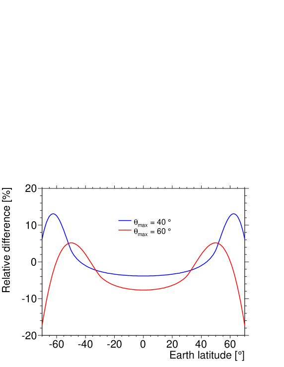
Figure 1: Relative differences between the mean hour angle and the factor $2\left<\sin\theta\right>/\pi\cos\ell\left<\cos\theta\right>$ as a function of the Earth latitude, for different conditions of maximal zenith angle available in the field of view.

Despite the crude approximations outlined in Section 2.2, it turns out that the factor $h_{\star}$ is not very different from the mean hour angle as long as the Earth latitude of the site of the experiment is smaller than 50^∘ in absolute value. This is illustrated in Fig. 1, where the relative difference $(\left<h\right>-h_{\star})/h_{\star}$ is shown as a function of the Earth latitude of the site, using $\epsilon(\theta,t)=1$ and two different values of $\theta_{max}$. It can be seen that these relative differences become larger than 10$\%$ only for Earth latitudes $\ell\geq 50^{\circ}$. The results would not be very different had we considered other examples of $\epsilon(\theta,t)$.

4 First Harmonic Analysis - Estimation of the dipole equatorial component

4.1 First Harmonic Analysis of $I_{E}-I_{W}$

To probe a dipolar structure of the CR arrival direction distribution, Eqn. 31 is an ideal starting point to estimate the dipolar modulation of $dI_{tot}^{true}/dt$ parameterised through the amplitude $r$ and the phase $\varphi$:

$$\frac{dI_{tot}^{true}(t)}{dt}=r\cos(t-\varphi).$$ (32)

From a set of $N$ arrival times from events coming from either the Eastern or the Western directions, $r$ and $\varphi$ can be estimated by applying to the arrival times of the events the standard first harmonic analysis [24] slightly modified to account for the subtraction of the Western sector to the Eastern one. The Fourier coefficients $a$ and $b$ are thus defined by:

$$a = \frac{2}{N}\sum_{i=1}^{N}\cos{(t_{i}+\zeta_{i})},$$ (33)

$$b = \frac{2}{N}\sum_{i=1}^{N}\sin{(t_{i}+\zeta_{i})},$$ (34)

where $\zeta_{i}$ equals 0 if the event is coming from the East or $\pi$ if coming from the West. The amplitude and phase estimates $(\hat{r},\hat{\varphi})$ of $dI_{tot}^{true}/dt$ are then obtained through:

$$\hat{r}=\frac{\pi\cos\ell}{2}\frac{\left<\cos\theta\right>}{\left<\sin\theta\right>}\sqrt{a^{2}+b^{2}}\\ \hskip 28.45274pt\mbox{and}\\ \hskip 28.45274pt\hat{\varphi}=\arctan\bigg{(}\frac{b}{a}\bigg{)}.$$ (35)

By integrating $dI/dt$, the amplitude and phase estimates $(\hat{r}_{I},\hat{\varphi}_{I})$ of the intensity $I(t)^{true}_{tot}$ itself are obtained:

$$\hat{r}_{I}=\frac{N}{2\pi}\hat{r}\\ \hskip 28.45274pt\mbox{and}\\ \hskip 28.45274pt\hat{\varphi}_{I}=\hat{\varphi}+\frac{\pi}{2}.$$ (36)

4.2 Estimation of the dipole equatorial component

In case of the standard Rayleigh analysis in right-ascension, the first harmonic amplitude $r$ is related to the dipole amplitude $D$ through [26]:

$$r_{RA}=\left|\frac{\left<\cos\delta\right>D_{\perp}}{1+\left<\sin\delta\right>D_{\parallel}}\right|,$$ (37)

where $D_{\parallel}=D\sin\delta_{d}$ denotes the component of the dipole along the Earth rotation axis while $D_{\perp}=D\cos\delta_{d}$ is the component in the equatorial plane. The first harmonic amplitude thus depends on the declination of the dipole in such a way that it vanishes for $\delta_{d}=\pm\pi/2$. This is obvious, as the modulation of the flux does not depend on the right ascension in such a case. On the other hand, the power of the method is the largest when the dipole is oriented in the equatorial plane. In this latter case the first harmonic amplitude becomes $r_{RA}=D_{\perp}\left<cos\delta\right>$ and the sensitivity of an experiment to the true value of $D_{\perp}$ depends then on $\left<\cos\delta\right>$, which is a function of the Earth latitude $\ell$ of the experiment and its detection efficiency in the zenithal range considered.

Similarly, the first harmonic amplitude reconstructed by the East-West method is not directly the dipole amplitude. The additional step consists in relating $dI_{tot}^{true}/dt$ and the dipolar parameters through measurable quantities. Remembering that the observed number of events $N$ is equal to $\int_{2\pi}dt(I_{E}^{obs}+I_{W}^{obs})=2\pi A\Phi_{0}\int_{2\pi}dt(g_{11}(t)+D_{z}(t)g_{21}(t))$ and that $D_{z}(t)=D\cos{\theta_{d}(t)}=D\left(\sin{\ell}\sin{\delta_{d}}+\cos{\ell}\cos{\delta_{d}}\cos{h_{d}(t)}\right)$, and neglecting all second order terms in $\eta D_{\perp}$ and $\eta D_{\parallel}$, Eqn. 30 can be rewritten as:

$$\frac{dI_{tot}^{true}(t)}{dt} \simeq -\frac{N}{2\pi}\frac{D_{\perp}\left<\cos\theta\right>\cos\ell\sin{h_{d}(t)}}{1+\frac{1}{2\pi}\int dt\,\eta(t)+D_{\parallel}\left<\cos\theta\right>\sin\ell}$$ (38)

This expression describes how a genuine dipole with amplitude $D$ and pointing to a declination $\delta_{d}$ modulates in time the intensity of CRs observed by a ground experiment located at an Earth latitude $\ell$. The amplitude of the time variation is suppressed if the dipole is approximately aligned with the Earth rotation axis, while the modulation is maximal if $D_{\parallel}$ is small compared to $D_{\perp}$. In this latter case the differential counting rate can thus be expressed as a function of the equatorial component of the dipole in a straightforward way:

$$I_{E}^{obs}(t)-I_{W}^{obs}(t)\simeq-\frac{N}{2\pi}\frac{2\left<\sin\theta\right>}{\pi}D_{\perp}\sin{h_{d}(t)},$$ (39)

where we have neglected the second order terms proportional to $\eta D_{\perp}$ and $D_{\parallel}D_{\perp}$.

The first harmonic amplitude and phase estimates $(\hat{D}_{\perp},\hat{\alpha}_{d})$ are thus obtained through:

$$\hat{D}_{\perp}=\frac{\hat{r}}{\cos\ell\left<\cos\theta\right>}=\frac{\pi}{2\left<\sin\theta\right>}\sqrt{a^{2}+b^{2}}\\ \hskip 28.45274pt\mbox{and}\\ \hskip 28.45274pt\hat{\alpha}_{d}=\hat{\varphi}+\frac{\pi}{2}.$$ (40)

It is worth noting that, from the transformation of coordinates relation $\cos\delta\sin{h}=-\sin\theta\cos\varphi$, the factor $2\left<\sin\theta\right>/\pi$ can be expressed as well in terms of $\delta$ and $h$ as:

$$\frac{2\left<\sin\theta\right>}{\pi}=\left<\cos\delta\sin{h}\right>,$$ (41)

where the r.h.s. average is performed by integrating over the eastern and western quadrants.

By comparing Eqn. 40 to Eqn. 37 and using Eqn. 41, it can be seen that the use of the local sidereal time in the modulation search (instead of the right ascension as in the case of the standard Rayleigh analysis), combined to the East-West subtraction, leads to a loss of sensitivity by a factor $\left<\cos\delta\right>/\left<\cos\delta\sin{h}\right>$ (which is typically about two, depending on the experimental conditions) with respect to the performances of the standard Rayleigh analysis. However, this method has the benefit of avoiding the need to implement any corrections of the total counting rates for instrumental and atmospheric effects. Moreover, in some cases those corrections cannot be computed reliably, for instance when they are due to the energy dependence of the trigger efficiency, which can also depend on the unknown composition of the primary CRs. In these cases, only the East-West method can be implemented reliably.

5 Simulations

In this section, we check the behavior of the method through simulations reproducing realistic conditions of a ground experiment subject to artificial modulations at both the diurnal and the seasonal time scales. For this purpose, we consider three typical cases of interest for this kind of studies:

• isotropy;

• genuine sidereal modulation;

• genuine solar modulation.

An additional underlying distribution has been considered to study the impact of a broken East-West symmetry:

• isotropy with a broken East-West symmetry.

In order to test extreme situations we also add the spurious effects to all of these distributions.

For definiteness we consider an experiment located at the same Earth latitude $\ell=-$35.25^∘ as the Pierre Auger Observatory [23] and sensitive up to a maximal zenith angle of 60^∘, with the following energy independent detection efficiency function:

$$\epsilon(\theta,t)=\frac{1}{1+\exp((\theta-\theta_{ns})/\sigma_{ns})}\cdot g(t),$$ (42)

where $\theta_{ns}=50^{\circ}$ and $\sigma_{ns}=5^{\circ}$. Here, $g(t)$ stands for the spurious modulation, which may differ from unity due to various reasons. For instance, the changes of atmospheric conditions affect the energy estimate of the showers [25]. When such effects are not accounted for, they induce a modulation of the rate of events above any given energy threshold. Hence, we choose the function $g(t)$ to be of the generic form [27]:

$$g(t)=\frac{1+\eta_{y}\cos(2\pi(t-t^{0}_{y})/T_{y})+\eta_{d}\bigg{[}1+\eta_{\star}\cos(2\pi(t-t^{0}_{y})/T_{y})\bigg{]}\cos(2\pi(t-t^{0}_{d})/T_{d})}{1+\eta_{y}+\eta_{d}(1+\eta_{\star})},$$ (43)

where $t$ is here expressed in terms of solar time. The cosine proportional to $\eta_{y}$ describes the annual variation of the mean event rate, with phase $t^{0}_{y}$ and a period $T_{y}$ of one year. The cosine proportional to $\eta_{d}$ describes the annual average of the solar diurnal modulation, with phase $t^{0}_{d}$ and a period $T_{d}$ of one day. Finally, $\eta_{\star}$ stands for the variation of the diurnal amplitude along the year. This last term, combining the diurnal modulation with an annual one, is responsible for the production of sidebands at both the sidereal and the anti-sidereal frequencies, whose amplitudes are given by $0.5\times\eta_{d}\times\eta_{\star}$ [27]. To illustrate the power of the East-West method, we choose an extremely high value of $\eta_{\star}=90\%$ to guarantee the existence of significant sidebands, while we set $\eta_{y}=20\%$ and $\eta_{d}=15\%$.

5.1 Case 1: isotropy with spurious effects

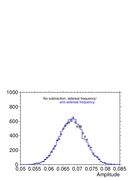
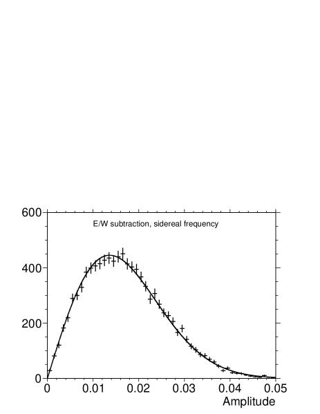
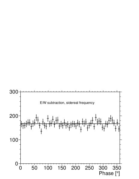
Figure 2: Top: Distributions of the amplitudes of the first harmonic obtained with the standard Rayleigh analysis in the presence of experimental effects in solar time ($a$) and in both sidereal and anti-sidereal times ($b$). Middle and Bottom: Distributions of the amplitudes ($c$ and $d$) and phases ($e$ and $f$) of the first harmonic obtained with the East-West analysis, compared with the isotropic expectations: the subtraction of the spurious effects holds perfectly.

We first consider an isotropic distribution of CRs polluted by the spurious effects described above, and analyse $10^{4}$ mock samples generated with a total number of events $N=10^{5}$. The net results of the instrumental and atmospheric effects introduced by the function $g(t)$ are shown on top of Fig. 2, evidencing that the net counting rate $I^{obs}_{tot}=I^{obs}_{E}+I^{obs}_{W}$ undergoes the expected modulation of amplitude $\eta_{d}=15\%$ at the solar frequency and of $0.5\times\eta_{d}\times\eta_{\star}=6.75\%$ at both the sidereal and the anti-sidereal frequencies. Applying the East-West analysis at both the solar and sidereal frequencies, it can be seen that the reconstructed amplitudes $\hat{D}_{\perp}$ and phases $\hat{\alpha}_{d}$ are now distributed according to the expected distributions: the Rayleigh one for the amplitude with parameter $\sigma=\pi/2\left<\sin\theta\right>\sqrt{2/N}$, and the uniform one for the phase. Hence, in spite of the strong experimental effects, it turns out that the East-West subtraction allows the removal of possible biases in the estimate of both the amplitude and phase in the case of an underlying isotropic distribution of CRs.

5.2 Case 2: 5% sidereal signal with spurious effects on the acceptance

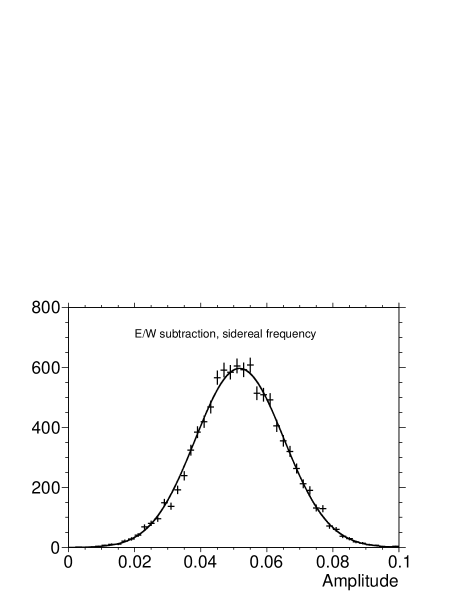
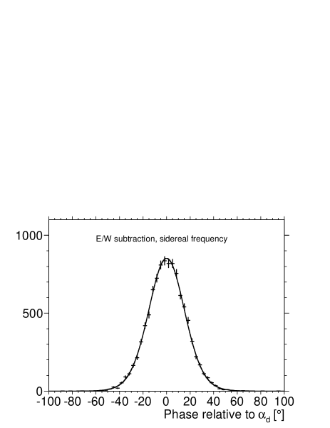
Figure 3: Distributions of the amplitudes ($a$) and phases ($b$) of the first harmonic in local sidereal time obtained with the East-West analysis in the presence of a genuine pattern of $5$%. Both histograms are in perfect agreement with respect to the expectations.

To test now the accuracy of the method in the presence of both a genuine signal at the sidereal frequency and spurious effects, a signal corresponding to a dipolar anisotropy of 5% amplitude is introduced in the simulated samples. For definiteness, we consider the dipole oriented towards the equatorial plane. The reconstructed amplitudes are now expected to follow a Rice distribution with parameters $\mu=5\%$ and $\sigma=\pi/2\left<\sin\theta\right>\sqrt{2/N}$:

$$p_{1}(\hat{D}_{\perp})=\frac{\hat{D}_{\perp}}{\sigma^{2}}\exp{\bigg{(}-\frac{\hat{D}_{\perp}^{2}+\mu^{2}}{2\sigma^{2}}\bigg{)}}I_{0}\bigg{(}\frac{\hat{D}_{\perp}\mu}{\sigma^{2}}\bigg{)},$$ (44)

while the reconstructed phases are expected to follow the distribution described by Linsley in the 2^nd alternative in [24]:

$$p_{2}(\hat{\alpha}_{d})=\frac{1}{2\pi}\exp{\bigg{(}-\frac{\mu^{2}}{2\sigma^{2}}}\bigg{)}+\frac{\mu\cos{(\hat{\alpha}_{d}-\alpha_{d})}}{2\sqrt{2\pi}\sigma}\bigg{(}1+\mathrm{erf}{\bigg{(}\frac{\mu\cos{(\hat{\alpha}_{d}-\alpha_{d})}}{\sqrt{2}\sigma}\bigg{)}}\bigg{)}\exp{\bigg{(}-\frac{\mu^{2}\sin^{2}{(\hat{\alpha}_{d}-\alpha_{d})}}{2\sigma^{2}}\bigg{)}},$$ (45)

The results of the simulations are shown in Fig. 3, evidencing a perfect agreement with the expectations.

5.3 Case 3: $0.1$% solar signal with spurious effects

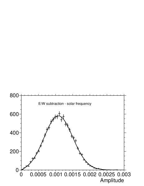
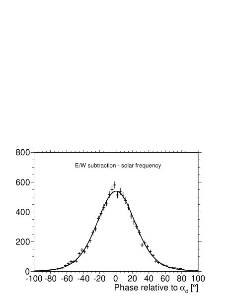
Figure 4: Same as Fig. 3, but generating a genuine pattern at the solar frequency.

We repeat here exactly the same exercise as above, but generating a genuine dipole with an amplitude $0.1$% at the solar frequency, together with the spurious effects. This kind of feature is expected due to the motion of the terrestrial observer through the frame in which the CR distribution is isotropic. It has been observed by several experiments at low energies, where sufficient statistics has been gathered. To probe such a low amplitude, the number of events has to be greatly increased with respect to the previous cases. Thus, we generated $10^{3}$ samples of $N=10^{8}$ events. The results of the simulations are shown in Fig. 4, showing once again perfect agreement with the expectations, even if both the genuine and the artificial modulations are present at the same time scale.

5.4 Case 4: isotropy with spurious effects and a broken East-West symmetry

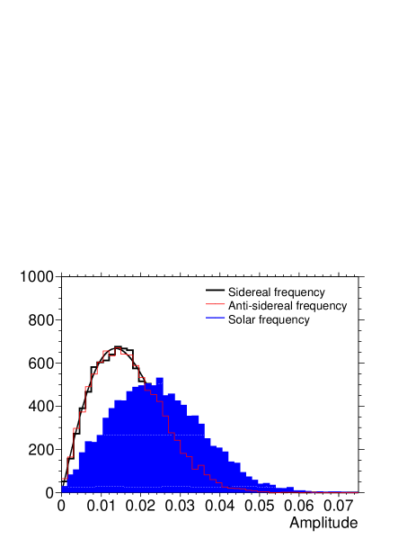
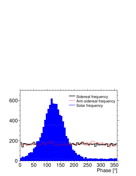
Figure 5: Distribution of the amplitudes $(a)$ and phases $(b)$ of the first harmonic obtained with the East-West analysis in case of isotropy and of a broken East-West symmetry of the detection efficiency of the experiment. Thick histogram: sidereal frequency. Thin histogram: anti-sidereal frequency. Filled histogram: solar frequency.

Finally, we study in this sub-section the influence of a broken East-West symmetry of the detection efficiency of a ground array experiment. There are several reasons in practice why the East-West symmetry may be slightly broken. We consider here an array being slightly tilted, the tilt being specified by a unit vector $\hat{n}$ described by its zenith angle $\gamma$ (the tilt) and its azimuth angle $\phi_{0}$ (the direction). If the unit vector $\hat{d}$ describes a given direction in the sky with zenith $\theta$ and azimuth $\phi$ the directional detection efficiency towards that direction is proportional to $\hat{d}\cdot\hat{n}$:

$$\hat{d}\cdot\hat{n}=\cos\gamma\cos\theta+\sin\gamma\sin\theta\cos(\phi-\phi_{0})\simeq\cos\theta\,\left[1+\gamma\tan\theta\cos(\phi-\phi_{0})\right].$$ (46)

Introducing this azimuthal dependence into the detection efficiency results in a small difference between the Eastward and Westward counting rates, proportional to $\gamma\cos{\phi_{0}}$ at first order in such a way that for any North/South asymmetry the effect cancels exactly. Meanwhile, being independent of time, this shift does not impact itself in the estimate of the first harmonic. However, it is worth examining the effect of the combination of the tilted array together with the modulations induced by weather effects on EAS developments, because this combination leads to an East-West counting rate proportional to $\gamma\eta(t)\cos{\phi_{0}}$, which may mimic a real East-West first harmonic modulation at the solar frequency.

Generating $10^{5}$ isotropic samples of $N=10^{4}$ events on a tilted ground array with a large value $\gamma=5^{\circ}$ and in the direction $\phi_{0}=0^{\circ}$ (leading to the maximal effect), we show in Fig. 5 the results obtained at the sidereal frequency (thick histogram), the anti-sidereal frequency (thin histogram), and the solar frequency (filled histogram). It is clear that in such a case, only the solar frequency is affected by the East-West asymmetry introduced by the tilted array. On the contrary, the analyses performed at the sidereal frequency remains unbiased.

6 Conclusions

The differential East-West method for the measurement of large scale anisotropies has been revisited. Using the fact that the experimental instabilities simultaneously affect both the East and the West sectors, we have shown that with this method the equatorial component of the dipole can be recovered in an unbiased way, without applying any corrections to account for spurious effects, but with a reduced sensitivity with respect to the standard Rayleigh analysis. Despite of this reduced sensitivity, this method has the advantage of avoiding the need to correct the total counting rate for instrumental and atmospheric effects. Finally, we have also shown that this method leads to unbiased results at the sidereal frequency even in the case of a broken East-West symmetry.

This article is devoted to the memory of Gianni Navarra. Besides being a great scientist, he was deeply involved in this analysis and was the real inspirer of this work.

References

- Nagashima et al. [1989] K. Nagashima et al. 1989, Il Nuovo Cimento C, 12, 695
- Gombosi et al. [1975] T. Gombosi et al. 1975, Nature, 255, 687
- Fenton et al. [1975] B.K. Fenton et al. 1975, Proc. 14th ICRC, 4, 1482
- Alekseenko et al. [1981] V.V. Alekseenko et al. 1981, Proc. 17th ICRC, 1, 146
- Andreev et al. [1987] Y. Andreev et al. 1987, Proc. 20th ICRC, 2, 22
- Ambrosio et al. [2003] M. Ambrosio et al. 2003, Phys. Rev. D, 67, 042002
- Munakata et al. [1997] K. Munakata et al 1997, Phys. Rev. D, 56, 23
- Amenomori et al. [2005] M. Amenomori et al. 2005, Ap. J., 626, L29
- Guillian et al. [2007] G. Guillian et al. 2007, Phys. Rev. D, 75, 062003
- Abdo et al. [2008] A.A. Abdo et al. 2009, Ap. J., 698, 2121
- Aglietta et al. [1996] M. Aglietta et al. 1996, Ap. J., 470, 501
- Kifune et al. [1984] T. Kifune et al. 1984, J. Phys. G, 12, 129
- Gherardy et al. [1983] P. Gerhardy et al. 1983, J. Phys. G, 9, 1279
- Antoni et al. [2004] T. Antoni et al. 2004, Ap. J., 604, 687
- Amenomori et al. [2006] M. Amenomori et al. 2006, Science, 314, 439
- Over et al. [2007] S. Over et al. 2007, Proc. 30th ICRC
- Aglietta et al. [2009] M. Aglietta et al. 2009, Ap. J. Lett., 692, L130
- [18] N. Hayashida et al. 1999, Astropart. Phys., 10, 303-311
- [19] D.J. Bird et al (Fly’s Eye Coll.) 1999, Ap. J., 511, 739
- [20] J.A. Bellido et al (SUGAR Coll.) 2001, Astropart. Phys., 15, 167
- [21] R. Bonino for the Pierre Auger Collaboration 2009, Proc. 31st ICRC, HE.1.4 35
- [22] The Pierre Auger Collaboration 2011, Astropart. Phys., 34, 627-639
- [23] The Pierre Auger Collaboration 2004, Nucl. Instr. and Meth., A523 , 50
- [24] J. Linsley 1975, Phys. Rev. Lett., 34, 1530-1533
- [25] The Pierre Auger Collaboration 2009, Astropart. Phys., 32, 89-99
- [26] J. Aublin and E. Parizot 2005, Astron. & Astrophys. 441, 407-415
- [27] F.J.M. Farley and J.R. Storey 1954, Proc. Phys. Soc. A, 67, 996-1004