Study of $\bar{B}^{0}\to D^{0}\mu^{+}\mu^{-}$ Decay in Perturbative QCD Approach

Abstract

Within the perturbative QCD approach and ignoring the contributions of long distance and subleading penguin loops, we investigate $\bar{B}^{0}\to D^{0}\mu^{+}\mu^{-}$ decay in the large recoiling kinematic region in the Standard Model. At the tree level, $\bar{B}^{0}$ decays to $D^{0}$ by exchanging a $W$ boson accompanied by a virtual photon emission from the valence quarks of $\bar{B}^{0}$ and $D^{0}$ meson, then the virtual photon decays to the lepton pair. Numerically, we find that the branching ratio decreases rapidly as the $q^{2}$ increases, and the branching ratio of $\bar{B}^{0}\to D^{0}\mu^{+}\mu^{-}$ is $(9.7_{-3.2}^{+4.2})\times 10^{-6}$ in the region $q^{2}\in[1,5]~{}\mathrm{GeV}^{2}$. The order of the branching ratio shows a possibility to study this interesting channel in the current $B$ factories and the Large Hadron Collider. The precise experimental data will help us to test the factorization approach and the QCD theory, in general.

Over the past few years when studying the semileptonic decays of $B$ meson, people always pay much attention on exclusive processes $B\to(K,K^{*},\pi,\rho)\ell^{+}\ell^{-}$ and inclusive processes $B\to X_{s,d}\ell^{+}\ell^{-}$ as well as similar decay modes, which are induced by the flavor changing neutral current $b\to s\ell^{+}\ell^{-}$ or $b\to d\ell^{+}\ell^{-}$. In these processes, the leptons are always generated from either a photon or a $Z$ boson with loop diagrams, so that these decay processes are considered as good choices of testing the Standard Model (SM) and probing possible new physics signals. Recent review in detail is referred to Refs. [1, 2, 3]. In fact when we study the decays $B\to(K,K^{*},\pi,\rho)\ell^{+}\ell^{-}$, the weak annihilation contributions are usually ignored since they are regarded to be suppressed by $\mathcal{O}(\Lambda_{QCD}/m_{B})$ [4]. Therefore, we think that it is of urgent interest to explore the pure annihilation type semileptonic $B$ meson decays, in which $\mathcal{O}(\Lambda_{QCD}/m_{B})$ effects are the main contribution. Still due to suppression of $\mathcal{O}(\Lambda_{QCD}/m_{B})$, most of these decays have small branching ratios, and cannot be observed in the current BaBar and Belle experiments. However, for some special decays, such as $\bar{B}^{0}\to D^{0}\mu^{+}\mu^{-}$, its branching ratio can be enhanced by large Wilson coefficients. In this work, we consider the observables of the decay $\bar{B}^{0}\to D^{0}\mu^{+}\mu^{-}$ theoretically. Compared with the mass of $B$ meson, both the masses of muon and electron are very small, so the analysis of $\bar{B}^{0}\to D^{0}e^{+}e^{-}$ is almost the same as $\bar{B}^{0}\to D^{0}\mu^{+}\mu^{-}$.

In the SM for $\bar{B}^{0}\to D^{0}\mu^{+}\mu^{-}$ the muon pair can be generated from either a photon or a $Z$ boson, however, the latter case will be highly suppressed because of the weak coupling and the large $Z$ mass. Therefore, we only consider the process where the lepton pair is generated from a virtual photon. In the full theory, there are three possible contributions to this decay, and we draw the Feynman diagrams in Fig. 1. In the first case, shown in diagram 1(a), $\bar{B}^{0}$ decays to $D^{0}+J/\psi$ by exchanging a $W$ boson and generating $c\bar{c}$ pair from the vacuum, in which the $J/\psi$ decays to lepton pair, which is so-called the resonant contribution. Because the mode $\bar{B}^{0}\to D^{0}+J/\psi(\to\ell^{+}\ell^{-})$ has not been observed yet, we will exclude this part of contribution, $i.e.$ Fig. 1(a), by carrying out our investigation in a certain kinematics region, $q^{2}\ll m_{J/\psi}^{2}$. The virtual photon can also be generated by the penguin operator $O_{7\gamma}^{s}$ or $O_{7\gamma}^{d}$, which is shown in diagram 1(b), with the Wilson coefficient $C_{7}$. Since this operator is from the loop suppressed flavor changing neutral current, the value of $C_{7}$ is much smaller than those of the coefficients $C_{1,2}$ of tree operators, and thus only marginally affecting our numerical estimates. Therefore, the contribution of diagram 1(b) has been neglected safely in this work. In diagram 1(c), the $B$ meson decays to a $D$ meson by exchanging a $W$ boson, where the photon can be emitted from either of the five crosses in diagram. When a photon is emitted from the $W$ boson, the diagram will be highly suppressed by the two $W$ propagators and because of the large $W$ mass. Therefore, we ignore this contribution in our calculation, too. Since this process happens at the scale ${\cal O}(m_{B})$, the highly off-shelled $W$ boson can be integrated out and the effective theory could be used directly, as shown in Fig. 2.

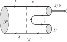
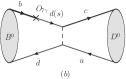
Figure 1: The possible diagrams for $B^{0}\to D^{0}\ell^{+}\ell^{-}$, where the crosses stand for a virtual photon.

To make predictions clear, one requires the knowledge of the matrix element $\langle D\gamma^{*}|B\rangle$, where the virtual photon $\gamma^{*}$ decays to a lepton pair. Although the calculation of this matrix is not trivial, it has been explored in many approaches, such as the heavy quark effective theory [5], the heavy light chiral perturbation theory [6], the QCD factorization approach [7] and the perturbative QCD (pQCD) approach [8]. Based on $k_{T}$ factorization, the pQCD approach [9, 10] is one of the theoretical instruments for handling such exclusive decay modes. The concept of pQCD is the factorization between soft and hard dynamics. In this approach, the quark transverse momentum $k_{T}$ is kept in order to eliminate the end-point singularity. Because of inclusion of transverse momenta, double logarithms from the overlap of two types of infrared divergences, soft and collinear, are generated in radiative corrections. The resummation of these double logarithms leads to a Sudakov factor, which suppresses the long-distance contribution. Though there still exist few controversies [11, 12] on its feasibility, the predictions based on the pQCD can accommodate experimental data well, for example, see Ref. [13]. In this work, we will put the controversies aside and adopt this approach to our analysis.

In the SM, the effective Hamiltonian related to decay $\bar{B}^{0}\to D^{0}\ell^{+}\ell^{-}$ is given [14] as:

$${\cal H}_{\rm{eff}}=\frac{G_{F}}{\sqrt{2}}V_{cb}V^{*}_{ud}\left[C_{1}(\mu)O_{1}(\mu)+C_{2}(\mu)O_{2}(\mu)\right],$$ (1)

where $G_{F}$ is the Fermi constant and $V_{cb}V^{*}_{ud}$ are the corresponding CKM matrix elements. $O_{1}$ and $O_{2}$ are local operators, which are defined as:

$$O_{1} = (\bar{c}_{\alpha}b_{\beta})_{V-A}(\bar{d}_{\beta}u_{\alpha})_{V-A}\;\;,$$

$$O_{2} = (\bar{c}_{\alpha}b_{\alpha})_{V-A}(\bar{d}_{\beta}u_{\beta})_{V-A}\;\;.$$ (2)

Here $\alpha$, $\beta$ are the color indices, $(\bar{q}_{1}q_{2})_{V-A}\equiv\bar{q}_{1}\gamma^{\mu}(1-\gamma^{5})q_{2}$, and $C_{1}$ and $C_{2}$ are corresponding Wilson coefficients, whose scale evolves from $m_{W}$ to the factorization scale $t$. With the Hamiltonian in Eq. (1), we draw the diagram in Fig. 2.

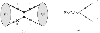
Figure 2: Diagram for $B^{0}\to D\ell^{+}\ell^{-}$ in the effective theory. The black boxes represent the effective vertex.

Now, we turn to discuss the decay $\bar{B}^{0}\to D^{0}\mu^{+}\mu^{-}$ in certain kinematic regions like $V_{\rm{start}}<q^{2}<V_{\rm{end}}$, where $q$ is the momentum of the $\ell^{+}\ell^{-}$ pair, $V_{\rm{start}}$ and $V_{\rm{end}}$ are the boundaries of the region. To guarantee our calculation reliable, we should choose the region where $D$ meson recoils fast and it can be treated on or nearly on the light cone. In the rest frame of $B$ meson, the momenta of $B$ and $D$ mesons are defined in the light-cone coordinate as

$$p_{B}=\frac{m_{B}}{\sqrt{2}}(1,1,\vec{0}_{\perp})\;,\;p_{D}=\frac{m_{D}}{\sqrt{2}}(\eta+\sqrt{\eta^{2}-1},\eta-\sqrt{\eta^{2}-1},\vec{0}_{\perp})\;,$$ (3)

with

$$\frac{m_{B}^{2}+m_{D}^{2}-V_{\rm{end}}}{2m_{B}m_{D}}<\eta<\frac{m_{B}^{2}+m_{D}^{2}-V_{\rm{start}}}{2m_{B}m_{D}}.$$ (4)

For the light quarks in $B$ and $D$ mesons, we define their momenta as

$$k_{1}=(0,\frac{m_{B}}{\sqrt{2}}x_{1},\vec{k}_{1\perp}),\;~{}~{}~{}k_{2}=(\frac{\eta+\sqrt{\eta^{2}-1}}{\sqrt{2}}x_{2}m_{D},0,\vec{k}_{2\perp})\;,$$ (5)

where $\vec{k}_{\perp}$ stands for the transverse momentum.

For the decay $\bar{B}^{0}\to D^{0}\ell^{+}\ell^{-}$ the amplitude will be factorized conventionally to a hadronic part and an electromagnetic part. To make our expressions simple, we parameterize the hadronic matrix element with two contracted weak vertices and one QED vertex as

$${T}^{\mu}=\langle D^{0}|C_{i}(\mu)O_{i}(\mu)\;\;\frac{(Ie_{l}g)(-I)(Ie_{q}g)\bar{q}\gamma^{\mu}q}{q^{2}}|\bar{B}^{0}\rangle=f_{1}(q^{2})p_{B}^{\mu}+f_{2}(q^{2})p_{D}^{\mu}~{},$$ (6)

where $f_{1}(q^{2})$ and $f_{2}(q^{2})$ are form factors, and their expressions are given by

$$f_{1}(q^{2}) = f_{1,1}(q^{2})+f_{1,2}(q^{2})+f_{1,3}(q^{2})+f_{1,4}(q^{2})\;,\;$$

$$f_{2}(q^{2}) = f_{2,1}(q^{2})+f_{2,2}(q^{2})+f_{2,3}(q^{2})+f_{2,4}(q^{2})\;,$$ (7)

in which the second subscripts of $f_{i,j}$ correspond to the numbers of the crosses in Fig. 2. Within the perturbative QCD approach, in the large recoiling region, $f_{i,j}$ could be calculated at the leading order up to the leading power of $m_{D}/m_{B}$. The detailed expressions are given in Appendix A. Unlike the form factors of the charged current process $\bar{B}^{0}\to D^{-}$, $f_{1}$ and $f_{2}$ are complex numbers, which are caused by the annihilation mechanism. Numerical results in the region $q^{2}\in[1\rm{GeV}^{2},5\rm{GeV}^{2}]$ show that both the real and imaginary parts of $f_{1}$ are much larger than those of $f_{2}$.

With the functions defined above, the amplitude can be expressed as

$${\cal M}=\frac{G_{F}}{\sqrt{2}}V_{cb}V^{*}_{ud}{T}^{\mu}[\bar{l}\gamma_{\mu}l]=f_{1}(q^{2})[\bar{l}\not p_{B}l]+f_{2}(q^{2})[\bar{l}\not p_{D}l],$$ (8)

and

$$|{\cal M}|^{2} = \frac{G_{F}^{2}}{2}|V_{cb}V^{*}_{ud}|^{2}\left[|f_{1}(q^{2})|^{2}{S}_{11}+|f_{2}(q^{2})|^{2}{S}_{22}+f_{1}(q^{2})f_{2}^{*}(q^{2}){S}_{12}+f_{1}^{*}(q^{2})f_{2}(q^{2}){S}_{21}\right]$$ (9)

with

$${S}_{11}=Tr[(\not p_{1}+m_{l})\not p_{B}(\not p_{2}-m_{l})\not p_{B}],$$

$${S}_{12}=Tr[(\not p_{1}+m_{l})\not p_{B}(\not p_{2}-m_{l})\not p_{D}],$$

$${S}_{21}=Tr[(\not p_{1}+m_{l})\not p_{D}(\not p_{2}-m_{l})\not p_{B}],$$

$${S}_{22}=Tr[(\not p_{1}+m_{l})\not p_{D}(\not p_{2}-m_{l})\not p_{D}].$$ (10)

In the above functions, $p_{1}$ and $p_{2}$ are the momenta of the $l^{-}$ and $l^{+}$ leptons respectively, and $m_{l}$ is the lepton mass. In the center of mass frame for the lepton pair, we define $p_{1}^{\prime}$ and $p_{2}^{\prime}$ as corresponding momenta of $p_{1}$ and $p_{2}$,

$$p_{1}^{\prime} = (\sqrt{q^{2}}/2,p\sin\theta\cos\phi,p\sin\theta\sin\phi,p\cos\theta),$$

$$p_{2}^{\prime} = (\sqrt{q^{2}}/2,-p\sin\theta\cos\phi,-p\sin\theta\sin\phi,-p\cos\theta),$$ (11)

where $p$ is the magnitude of $3$-component momentum and $p^{2}=q^{2}/4-m_{l}^{2}$, $\theta$[$\phi$] is the inclination [azimuth] coordinate of $l^{-}$. After the Lorentz transformation, one can get the expressions for $p_{1}$ and $p_{2}$ as follows.

$$p_{1} = (\gamma\sqrt{q^{2}}/2-\gamma\beta p\cos\theta,p\sin\theta\cos\phi,p\sin\theta\sin\phi,-\gamma\beta\sqrt{q^{2}}/2+\gamma p\cos\theta),$$

$$p_{2} = (\gamma\sqrt{q^{2}}/2+\gamma\beta p\cos\theta,-p\sin\theta\cos\phi,-p\sin\theta\sin\phi,-\gamma\beta\sqrt{q^{2}}/2-\gamma p\cos\theta),$$ (12)

where $\beta=\frac{m_{D}\sqrt{\eta^{2}-1}}{m_{B}-m_{D}\eta}$ and $\gamma=(1-\beta^{2})^{-1/2}$. As a consequence, the expressions for ${S}_{ij}$ with $i,j=1,2$ are given as

$${S}_{11} = m_{B}^{2}\left(4m_{l}^{2}\cos^{2}\theta+q^{2}\sin^{2}\theta\right)\left[-1+\gamma^{2}\left(1+\beta^{2}\right)\right],$$

$${S}_{12} = m_{B}m_{D}\left(4m_{l}^{2}\cos^{2}\theta+q^{2}\sin^{2}\theta\right)\left[-\eta+\eta\gamma^{2}\left(1+\beta^{2}\right)+2\beta\gamma^{2}\sqrt{\eta^{2}-1}\right],$$

$${S}_{21} = {S}_{12},$$

$${S}_{22} = m_{D}^{2}\left(4m_{l}^{2}\cos^{2}\theta+q^{2}\sin^{2}\theta\right)\left\{-1+\gamma^{2}\left[-1+2\eta^{2}+\beta^{2}\left(2\eta^{2}-1\right)+4\beta\eta\sqrt{\eta^{2}-1}\right]\right\}.$$ (13)

The most important inputs of the calculation are hadron distribution amplitudes, named $\phi_{B}$ and $\phi_{D}$, which contain the nonperturbative effects in the mesons under the scale $\Lambda_{QCD}$. Under the factorization frame, they are universal quantities and can be constrained from well measured decay channels. For the $B$ meson distribution amplitude, we adopt the model [9]:

$$\phi_{B}(x,b)=N_{B}x^{2}(1-x)^{2}\exp\left[-\frac{1}{2}\left(\frac{xM_{B}}{\omega_{B}}\right)^{2}-\frac{\omega_{B}^{2}b^{2}}{2}\right]\;,$$ (14)

with the shape parameter $\omega_{B}=0.40\pm 0.05$ GeV, which has been tested in many channels such as $B\to\pi\pi,K\pi$ [10]. The normalization constant $N_{B}$ is related to the decay constant $f_{B}=190$ MeV [9] by the normalization condition in Eq. (16). As for $D$ meson, the distribution amplitude, determined in Ref. [15] by fitting, is

$$\phi_{D}=\frac{1}{2\sqrt{6}}f_{D}6x(1-x)\left[1+C_{D}(1-2x)\right]\exp\left[-\frac{\omega^{2}b^{2}}{2}\right],$$ (15)

where $C_{D}=0.5,\omega=0.1$. Both distribution amplitudes are normalized as:

$$\int^{1}_{0}dx\phi_{M}(x)=\frac{f_{M}}{2\sqrt{2N_{C}}},\,\,\,M=B,D.$$ (16)

One can obtain the differential decay width by

$$\frac{d\Gamma}{dq^{2}d\cos\theta d\phi}=\frac{\sqrt{\lambda}}{1024\pi^{4}m_{B}^{3}}\sqrt{\frac{q^{2}-4m_{l}^{2}}{q^{2}}}|{\cal M}|^{2},$$ (17)

where $\lambda=(m_{B}^{2}+m_{D}^{2}-q^{2})^{2}-4m_{B}^{2}m_{D}^{2}$. Integrating over the angle variables, we would obtain the $q^{2}$-dependance of the decay width as well as the branching ratio. In Eq. (17), the factor $\sqrt{\frac{q^{2}-4m_{l}^{2}}{q^{2}}}$ ensures that the branching ratio at $q^{2}=4m_{l}^{2}$ vanishes, however, the $q^{2}$ appearing in the denominator of the photon propagator generates a pole-like structure at the small $q^{2}$ region. Since it is very difficult for the detector to observe leptons with such a low energy, we simply subtract the region with very small $q^{2}$ value. In addition, in order to avoid the pollution from long distance contributions shown in Fig 1(a), we set the maximum value of $q^{2}$ as $5~{}\mathrm{GeV}^{2}$.

In Fig. 3, we present the behavior of the branching ratio of this decay mode with $1~{}{\rm GeV}^{2}<q^{2}<5~{}{\rm GeV}^{2}$. From the figure, one can see that the value of the branching ratio decreases rapidly as the $q^{2}$ increases: at $q^{2}=1~{}\rm{GeV}^{2}$ the value is $3.2\times 10^{-5}$, and it decreases to $2.8\times 10^{-8}$ at $q^{2}=5~{}\rm{GeV}^{2}$. By integrating the branching ratio over $q^{2}$ in the region $[1,5]~{}\rm{GeV}^{2}$, we obtain:

$$BR(\bar{B}^{0}\to D^{0}\mu^{+}\mu^{-})=\left(9.7_{-3.2}^{+4.2}\right)\times 10^{-6},$$ (18)

where the errors are mainly from $\Lambda_{QCD}$. The errors from the decay constant are not listed directly, which are proportional to the square of the decay constants. We here do not discuss the uncertainties taken by CKM elements, simply because they can be measured well in other decay channels. Since there only vector currents appear in the calculation, there is no forward-backward asymmetry in this decay mode at the tree level, so any apparent deviation from zero would be the signal from new physics. The order of magnitude for branching ratio shows a possibility to study this channel in present Belle, BaBar and LHC-b as well as future Super-$B$ factories. The precise experimental data will help us to test the factorization approach, and the QCD theory itself in general. We are pretty sure that future studies on the decays will come soon from several other theoretical approaches, and the numerical estimates will be further refined.

Figure 3: The dependence of the branching ratio of $\bar{B}^{0}\to D^{0}\mu^{+}\mu^{-}$ with $q^{2}$, and $q^{2}\in[1,5]\rm{GeV}^{2}$.

Finally, let us summarize our work. Within the pQCD approach, we studied the exclusive rare decay of $\bar{B}^{0}\to D^{0}\mu^{+}\mu^{-}$, which is pure annihilation type decay. Explicitly, we have found that the branching ratio is $\left(9.7_{-3.2}^{+4.2}\right)\times 10^{-6}$ and the forward-backward asymmetry is zero at the tree level. It is clear that such an order of magnitude for branching ratio could be well measured at the ongoing $B$ factories and Large Hadron Collider as well as future Super-$B$ factories.

Appendix A Appendix A: Relevant Functions

The definitions of $f_{i,j}$ used in the text are presented in this appendix. These functions can be calculated directly within the perturbative QCD approach:

$$f_{1,1}(q^{2}) = 4e_{b}\pi\alpha_{\rm{em}}m_{D}f_{D}\int_{0}^{1}dx_{1}\int_{0}^{\rm{\Lambda_{\rm{QCD}}}}db_{1}b_{1}a_{2}(t_{1})\exp[-S_{B}(t_{1})]\phi_{B}(x_{1})\frac{\sqrt{6}}{(\eta^{2}-1)q^{2}\pi}H_{0}(\sqrt{D_{1}}b_{1})$$

$$\times\left(2m_{D}(4\eta^{4}-5\eta^{2}-3\eta\sqrt{\eta^{2}-1}+4\eta^{3}\sqrt{\eta^{2}-1}+1)-m_{B}(x_{1}-2)(2\eta^{3}+2\eta^{2}\sqrt{\eta^{2}-1}-\sqrt{\eta^{2}-1}-2\eta)\right),$$

$$f_{2,1}(q^{2}) = 4e_{b}\pi\alpha_{\rm{em}}m_{B}f_{D}\int_{0}^{1}dx_{1}\int_{0}^{\rm{\Lambda_{\rm{QCD}}}}db_{1}b_{1}a_{2}(t_{1})\exp[-S_{B}(t_{1})]\phi_{B}(x_{1})\frac{\sqrt{6}}{(\eta^{2}-1)q^{2}\pi}H_{0}(\sqrt{D_{1}}b_{1})$$

$$\times\left(m_{B}(x_{1}-2)(\eta^{2}+\eta\sqrt{\eta^{2}-1}-1)+2m_{D}(-2\eta^{3}-2\eta^{2}\sqrt{\eta^{2}-1}+\sqrt{\eta^{2}-1}+2\eta)\right),$$

$$f_{1,2}(q^{2}) = 4e_{d}\pi\alpha_{\rm{em}}m_{D}f_{D}\int_{0}^{1}dx_{1}\int_{0}^{\rm{\Lambda_{\rm{QCD}}}}db_{1}b_{1}a_{2}(t_{2})\exp[-S_{B}(t_{2})]\phi_{B}(x_{1})\frac{\sqrt{6}}{(\eta^{2}-1)q^{2}}$$

$$\times\left\{\begin{array}[]{l}\frac{1}{\pi}K_{0}(\sqrt{D_{2}}b_{1})\,\,\,\,\,\,\,\mbox{when}\,\,D_{2}>0\\ \frac{i}{2}H_{0}(\sqrt{|D_{2}|}b_{1})\,\,\,\mbox{when}\,\,D_{2}<0\end{array}\right\}$$

$$\times\left(2m_{D}(4\eta^{4}-5\eta^{2}-3\eta\sqrt{\eta^{2}-1}+4\eta^{3}\sqrt{\eta^{2}-1}+1)+m_{B}(x_{1}-2)(2\eta^{3}+2\eta^{2}\sqrt{\eta^{2}-1}-\sqrt{\eta^{2}-1}-2\eta)\right),$$

$$f_{2,2}(q^{2}) = -4e_{d}\pi\alpha_{\rm{em}}m_{B}f_{D}\int_{0}^{1}dx_{1}\int_{0}^{\rm{\Lambda_{\rm{QCD}}}}db_{1}b_{1}a_{2}(t_{2})\exp[-S_{B}(t_{2})]\phi_{B}(x_{1})\frac{\sqrt{6}}{(\eta^{2}-1)q^{2}}$$

$$\times\left\{\begin{array}[]{l}\frac{1}{\pi}K_{0}(\sqrt{D_{2}}b_{1})\,\,\,\,\,\,\,\mbox{when}\,\,D_{2}>0\\ \frac{i}{2}H_{0}(\sqrt{|D_{2}|}b_{1})\,\,\,\mbox{when}\,\,D_{2}<0\end{array}\right\}$$

$$\times\left(m_{B}(x_{1}-2)(\eta^{2}+\eta\sqrt{\eta^{2}-1}-1)+2m_{D}(2\eta^{3}+2\eta^{2}\sqrt{\eta^{2}-1}-\sqrt{\eta^{2}-1}-2\eta)\right),$$

$$f_{1,3}(q^{2}) = -4e_{c}\pi\alpha_{\rm{em}}m_{D}f_{B}\int_{0}^{1}dx_{2}\int_{0}^{\rm{\Lambda_{\rm{QCD}}}}db_{2}b_{2}a_{2}(t_{3})\exp[-S_{D}(t_{3})]\phi_{D}(x_{2})\frac{\sqrt{6}}{(\eta^{2}-1)q^{2}}$$

$$\times\left\{\begin{array}[]{l}\frac{1}{\pi}K_{0}(\sqrt{D_{3}}b_{2})\,\,\,\,\,\,\,\mbox{when}\,\,D_{3}>0\\ \frac{i}{2}H_{0}(\sqrt{|D_{3}|}b_{2})\,\,\,\mbox{when}\,\,D_{3}<0\end{array}\right\}\times\left(2m_{B}\left(-2\eta^{3}-2\eta^{2}\sqrt{\eta^{2}-1}+\sqrt{\eta^{2}-1}+2\eta\right)\right.$$

$$\left.+m_{D}\left(x_{2}(4\eta^{4}-5\eta^{2}-3\eta\sqrt{\eta^{2}-1}+4\eta^{3}\sqrt{\eta^{2}-1}+1)-2(\eta^{2}+\eta\sqrt{\eta^{2}-1}-1)\right)\right),$$

$$f_{2,3}(q^{2}) = -4e_{c}\pi\alpha_{\rm{em}}m_{B}f_{B}\int_{0}^{1}dx_{2}\int_{0}^{\rm{\Lambda_{\rm{QCD}}}}db_{2}b_{2}a_{2}(t_{3})\exp[-S_{D}(t_{3})]\phi_{D}(x_{2})\frac{\sqrt{6}}{(\eta^{2}-1)q^{2}}$$

$$\times\left\{\begin{array}[]{l}\frac{1}{\pi}K_{0}(\sqrt{D_{3}}b_{2})\,\,\,\,\,\,\,\mbox{when}\,\,D_{3}>0\\ \frac{i}{2}H_{0}(\sqrt{|D_{3}|}b_{2})\,\,\,\mbox{when}\,\,D_{3}<0\end{array}\right\}$$

$$\times\left(2m_{B}(\eta^{2}+\eta\sqrt{\eta^{2}-1}-1)+m_{D}\left(x_{2}(-2\eta^{3}-2\eta^{2}\sqrt{\eta^{2}-1}+\sqrt{\eta^{2}-1}+2\eta)+2\sqrt{\eta^{2}-1}\right)\right),$$

$$f_{1,4}(q^{2}) = -4e_{u}\pi\alpha_{\rm{em}}m_{D}f_{B}\int_{0}^{1}dx_{2}\int_{0}^{\rm{\Lambda_{\rm{QCD}}}}db_{2}b_{2}a_{2}(t_{4})\exp[-S_{D}(t_{4})]\phi_{D}(x_{2})\frac{i\sqrt{3}}{\sqrt{2}(\eta^{2}-1)q^{2}}H_{0}(\sqrt{D_{4}}b_{2})$$

$$\times\left(2m_{B}\left(2\eta^{3}+2\eta^{2}\sqrt{\eta^{2}-1}-\sqrt{\eta^{2}-1}-2\eta\right)+m_{D}(x_{2}-2)\left(4\eta^{4}-5\eta^{2}-3\eta\sqrt{\eta^{2}-1}+4\eta^{3}\sqrt{\eta^{2}-1}+1\right)\right),$$

$$f_{2,4}(q^{2}) = -4e_{u}\pi\alpha_{\rm{em}}m_{B}f_{B}\int_{0}^{1}dx_{2}\int_{0}^{\rm{\Lambda_{\rm{QCD}}}}db_{2}b_{2}a_{2}(t_{4})\exp[-S_{D}(t_{4})]\phi_{D}(x_{2})\frac{i\sqrt{3}}{\sqrt{2}(\eta^{2}-1)q^{2}}H_{0}(\sqrt{D_{4}}b_{2})$$ (31)

$$\times\left(-2m_{B}(\eta^{2}+\eta\sqrt{\eta^{2}-1}-1)-m_{D}(x_{2}-2)\left(2\eta^{3}+2\eta^{2}\sqrt{\eta^{2}-1}-\sqrt{\eta^{2}-1}-2\eta\right)\right),$$

where $H_{0}^{(1)}(z)=J_{0}(z)+i\,Y_{0}(z)$, and $J_{0},Y_{0}$ and $K_{0}$ are Bessel functions.

The expressions for $D_{i}$ ($i=1,2,3,4$) are given as

$$D_{1} = -m_{D}^{2}+m_{B}^{2}+m_{B}m_{D}x_{1}(\eta+\sqrt{\eta^{2}-1})\;,$$

$$D_{2} = -m_{B}^{2}(1-x_{1})-m_{D}^{2}-m_{B}m_{D}[-2\eta+x_{1}(\eta+\sqrt{\eta^{2}-1})],$$

$$D_{3} = -m_{B}^{2}+m_{D}^{2}+m_{B}m_{D}x_{2}(\eta+\sqrt{\eta^{2}-1}),$$

$$D_{4} = -m_{B}^{2}-2m_{D}^{2}+m_{B}m_{D}(\eta-\sqrt{\eta^{2}-1}).$$ (32)

The hard scale $t$’s in the amplitudes are taken as the largest energy scale in the hard kernel $H_{0}$ (or $K_{0}$): $t_{i}={\rm{max}}\left(\sqrt{|D_{i}|},1/b_{j}\right)$ with $j=1$ when $i=1,2$ and $j=2$ when $i=3,4$.

Functions, $S_{B}$ and $S_{D}$, result from summing both double logarithms caused by soft gluon corrections and singular ones due to the renormalization of ultra-violet divergence. $S_{B,D}$ are defined as

$$S_{B}(t)=s(x_{1}P_{1}^{+},b_{1})+2\int_{1/b_{1}}^{t}\frac{d\mu^{\prime}}{\mu^{\prime}}\gamma_{q}(\mu^{\prime}),$$ (33)

$$S_{D}(t)=s(x_{2}P_{2}^{+},b_{3})+2\int_{1/b_{2}}^{t}\frac{d\mu^{\prime}}{\mu^{\prime}}\gamma_{q}(\mu^{\prime}),$$ (34)

where $s(Q,b)$, so-called Sudakov factor, is given in [10] as

$$s(Q,b) = \int_{1/b}^{Q}\!\!\frac{d\mu^{\prime}}{\mu^{\prime}}\left[\left\{\frac{2}{3}(2\gamma_{E}-1-\log 2)+C_{F}\log\frac{Q}{\mu^{\prime}}\right\}\frac{\alpha_{s}(\mu^{\prime})}{\pi}\right.$$ (35)

$$\left.+\left\{\frac{67}{9}-\frac{\pi^{2}}{3}-\frac{10}{27}n_{f}+\frac{2}{3}\beta_{0}\log\frac{\gamma_{E}}{2}\right\}\left(\frac{\alpha_{s}(\mu^{\prime})}{\pi}\right)^{2}\log\frac{Q}{\mu^{\prime}}\right],$$

where $\gamma_{E}=0.57722\cdots$ is Euler constant, and $\gamma_{q}=\alpha_{s}/\pi$ is the quark anomalous dimension.

References

[1]
M. Antonelli et al.,
Phys. Rept. 494, 197 (2010)
[arXiv:0907.5386 [hep-ph]].
[2]
W. Altmannshofer, P. Ball, A. Bharucha, A. J. Buras, D. M. Straub and M. Wick,
JHEP 0901, 019 (2009)
[arXiv:0811.1214 [hep-ph]].
[3]
A. J. Buras,
arXiv:1102.5650 [hep-ph].
[4]
M. Beneke, T. Feldmann and D. Seidel,
Nucl. Phys. B 612, 25 (2001)
[arXiv:hep-ph/0106067].
[5]
O. Antipin and G. Valencia,
Phys. Rev. D 74, 054015 (2006)
[arXiv:hep-ph/0606065].
[6]
J. A. Macdonald Sorensen and J. O. Eeg,
Phys. Rev. D 75, 034015 (2007)
[arXiv:hep-ph/0605078].
[7]
N. Kivel,
arXiv:0708.2393 [hep-ph].
[8]
Y. Li and C. D. Lu,
Phys. Rev. D 74, 097502 (2006)
[arXiv:hep-ph/0605220].
[9]
Y. Y. Keum, H. n. Li and A. I. Sanda,
Phys. Lett. B 504, 6 (2001)
[arXiv:hep-ph/0004004].
[10]
Y. Y. Keum, H. N. Li and A. I. Sanda,
Phys. Rev. D 63, 054008 (2001)
[arXiv:hep-ph/0004173];
C. D. Lu, K. Ukai and M. Z. Yang,
Phys. Rev. D 63, 074009 (2001)
[arXiv:hep-ph/0004213];
A. Ali, G. Kramer, Y. Li, C. D. Lu, Y. L. Shen, W. Wang and Y. M. Wang,
Phys. Rev. D 76, 074018 (2007)
[arXiv:hep-ph/0703162].
[11]
S. Descotes-Genon and C. T. Sachrajda,
Nucl. Phys. B 625, 239 (2002)
[arXiv:hep-ph/0109260].
[12]
F. Feng, J. P. Ma and Q. Wang,
Phys. Lett. B 674, 176 (2009)
[arXiv:0807.0296 [hep-ph]];
H. n. Li and S. Mishima,
Phys. Lett. B 674, 182 (2009)
[arXiv:0808.1526 [hep-ph]];
F. Feng, J. P. Ma and Q. Wang,
Phys. Lett. B 677, 121 (2009)
[arXiv:0808.4017 [hep-ph]].
[13]
H. n. Li and S. Mishima,
Phys. Rev. D 71, 054025 (2005)
[arXiv:hep-ph/0411146];
H. n. Li, S. Mishima and A. I. Sanda,
Phys. Rev. D 72, 114005 (2005)
[arXiv:hep-ph/0508041];
H. n. Li and S. Mishima,
Phys. Rev. D 74, 094020 (2006)
[arXiv:hep-ph/0608277].
[14]
G. Buchalla, A. J. Buras and M. E. Lautenbacher,
Rev. Mod. Phys. 68, 1125 (1996)
[arXiv:hep-ph/9512380].
[15]
R. H. Li, C. D. Lu and H. Zou,
Phys. Rev. D 78, 014018 (2008)
[arXiv:0803.1073 [hep-ph]].