Endpoint distribution of directed polymers in $1+1$ dimensions

Abstract.

We give an explicit formula for the joint density of the max and argmax of the Airy₂ process minus a parabola. The argmax has a universal distribution which governs the rescaled endpoint for large time or temperature of directed polymers in $1+1$ dimensions.

1. Introduction

In geometric last passage percolation, one considers a family $\big{\{}w(i,j)\}_{i,j\in\mathbb{Z}^{+}}$ of independent geometric random variables with parameter $q$ (i.e. $\mathbb{P}(w(i,j)=m)=q(1-q)^{m}$ for $m\geq 0$) and lets $\Pi_{n}$ be the collection of up-right paths of length $n$, that is, paths $\pi=(\pi_{0},\dotsc,\pi_{n})$ such that $\pi_{i}-\pi_{i-1}\in\{(1,0),(0,1)\}$. The point-to-point last passage time is defined, for $m,n\in\mathbb{Z}^{+}$, by

$$L(m,n)=\max_{\pi\in\Pi_{m+n}:(0,0)\to(m,n)}\sum_{i=0}^{m+n}w(\pi(i)),$$

where the notation in the subscript in the maximum means all up-right paths connecting the origin to $(m,n)$. Next one defines the process $t\mapsto H_{n}(t)$ by linearly interpolating the values given by scaling $L(n,y)$ through the relation

$$L(n+y,n-y)=c_{1}n+c_{2}n^{1/3}H_{n}(c_{3}n^{-2/3}y),$$

where the constants $c_{i}$ have explicit expressions which depend only on $q$ and can be found in [Joh03]. The random variables

$$\mathcal{T}_{n}=\inf\big{\{}t\!:\sup_{s\leq t}H_{n}(s)=\sup_{s\in\mathbb{R}}H_{n}(s)\big{\}}$$

then correspond to the location of the endpoint of the maximizing path with unconstrained endpoint. [Joh03] showed that

(1.1) $$H_{n}(t)\to\mathcal{A}_{2}(t)-t^{2}$$

in distribution, in the topology of uniform convergence on compact sets, where $\mathcal{A}_{2}$ is the Airy₂ process, which is a universal limiting spatial fluctuation process in such models, and is defined through determinantal formulas for its finite-dimensional distributions (see the companion paper [CQR12] for a description). Together with known results for last passage percolation [BR01], Johansson’s result (see also [CQR12]) implies that

(1.2) $$\mathbb{P}\!\left(\sup_{t\in\mathbb{R}}\{\mathcal{A}_{2}(t)-t^{2}\}\leq m\right)=F_{\rm GOE}(4^{1/3}m),$$

where $F_{\rm GOE}$ is the Tracy-Widom largest eigenvalue distribution for the Gaussian Orthogonal Ensemble (GOE) from random matrix theory [TW96].

Now let $\mathcal{T}$ denote the location at which the maximum is attained,

$$\mathcal{T}=\operatorname*{arg\,max}_{t\in\mathbb{R}}\{\mathcal{A}_{2}(t)-t^{2}\}.$$

Together with the recent result of [CH11] that the supremum of $\mathcal{A}_{2}(t)-t^{2}$ is attained at a unique point, Theorem 1.6 of [Joh03] shows

Theorem 1.

As $n\to\infty$, $\mathcal{T}_{n}\to\mathcal{T}$ in distribution.

In this article we complete the picture by providing an explicit formula for the distribution of $\mathcal{T}$. Let $\mathcal{M}$ denote the maximum of the Airy₂ process minus a parabola

(1.3) $$\mathcal{M}=\max_{t\in\mathbb{R}}\{\mathcal{A}_{2}(t)-t^{2}\}.$$

Our main result is in fact an explicit formula (1.11) for the joint density $f(t,m)$ of $\mathcal{T}$ and $\mathcal{M}$.

In the derivation of the formula, we will assume the result of [CH11] that the maximum of $\mathcal{A}_{2}(t)-t^{2}$ is obtained at a unique point. However, we point out that it is not necessary to do this. In fact, if one follows the argument without this assumption, one ends up with a formula for what is in principle a super-probability density, i.e. a non-negative function $f(t,m)$ on $\mathbb{R}\times\mathbb{R}$ with $\int_{\mathbb{R}\times\mathbb{R}}dm\,dt\,f(t,m)\geq 1$, and in fact one can see from the argument that

(1.4) $$\int_{\mathbb{R}\times\mathbb{R}}dm\,dt\,f(t,m)={\rm expected~{}number~{}of~{}maxima~{}of~{}}\mathcal{A}_{2}(t)-t^{2}.$$

Recall that from (1.2) that the distribution of $\mathcal{M}$ is given by a scaled version of $F_{\rm GOE}$. A non-trivial computation (see Section 3) on the resulting $f(t,m)$ gives

(1.5) $$\int_{-\infty}^{\infty}dt\,f(t,m)=4^{1/3}F^{\prime}_{\mathrm{GOE}}(4^{1/3}m).$$

This shows that the resulting $f(t,m)$ has total integral one, which can only be true if the maximum is unique almost surely. Thus we provide an independent proof of the uniqueness of the maximum of $\mathcal{A}_{2}(t)-t^{2}$.

Now we state the formula. Let $B_{m}$ be the integral operator with kernel

(1.6) $$B_{m}(x,y)=\operatorname{Ai}(x+y+m).$$

Recall that [FS05] showed that $F_{\mathrm{GOE}}$ can be expressed as the determinant

(1.7) $$F_{\mathrm{GOE}}(m)=\det(I-P_{0}B_{m}P_{0}),$$

where $P_{a}$ denotes the projection onto the interval $[a,\infty)$ (the formula essentially goes back to [Sas05]). Here, and in everything that follows, the determinant means the Fredholm determinant in the Hilbert space $L^{2}(\mathbb{R})$. In particular, note that since $F_{\mathrm{GOE}}(m)>0$ for all $m\in\mathbb{R}$, (1.7) implies that $I-P_{0}B_{m}P_{0}$ is invertible. We will write

(1.8) $$\varrho_{m}(x,y)=(I-P_{0}B_{m}P_{0})^{-1}(x,y).$$

Also, for $t,m\in\mathbb{R}$ define the function

(1.9) $$\psi_{t,m}(x)=2e^{xt}\left[t\operatorname{Ai}(x+m+t^{2})+\operatorname{Ai}^{\prime}(x+m+t^{2})\right]$$

and the kernel

$$\Psi_{t,m}(x,y)=2^{1/3}\psi_{t,m}(2^{1/3}x)\psi_{-t,m}(2^{1/3}y).$$

Finally, let

(1.10) $$\gamma(t,m)=2^{1/3}\int_{0}^{\infty}dx\int_{0}^{\infty}dy\,\psi_{-t,4^{-1/3}m}(2^{1/3}x)\varrho_{m}(x,y)\psi_{t,4^{-1/3}m}(2^{1/3}y).$$

Theorem 2.

The joint density $f(t,m)$ of $\mathcal{T}$ and $\mathcal{M}$ is given by

(1.11) $$\begin{split}f(t,m)&=\gamma(t,4^{1/3}m)F_{\mathrm{GOE}}(4^{1/3}m)\\ &=\det\!\big{(}I-P_{0}B_{4^{1/3}m}P_{0}+P_{0}\Psi_{t,m}P_{0}\big{)}-F_{\mathrm{GOE}}(4^{1/3}m).\end{split}$$

Integrating over $m$ one obtains a formula for the probability density $f_{\rm end}(t)$ of $\mathcal{T}$. Unfortunately, it does not appear that the resulting integral can be calculated explicitly, so the best formula one has is

(1.12) $$f_{\rm end}(t)=\int_{-\infty}^{\infty}dm\,f(t,m).$$

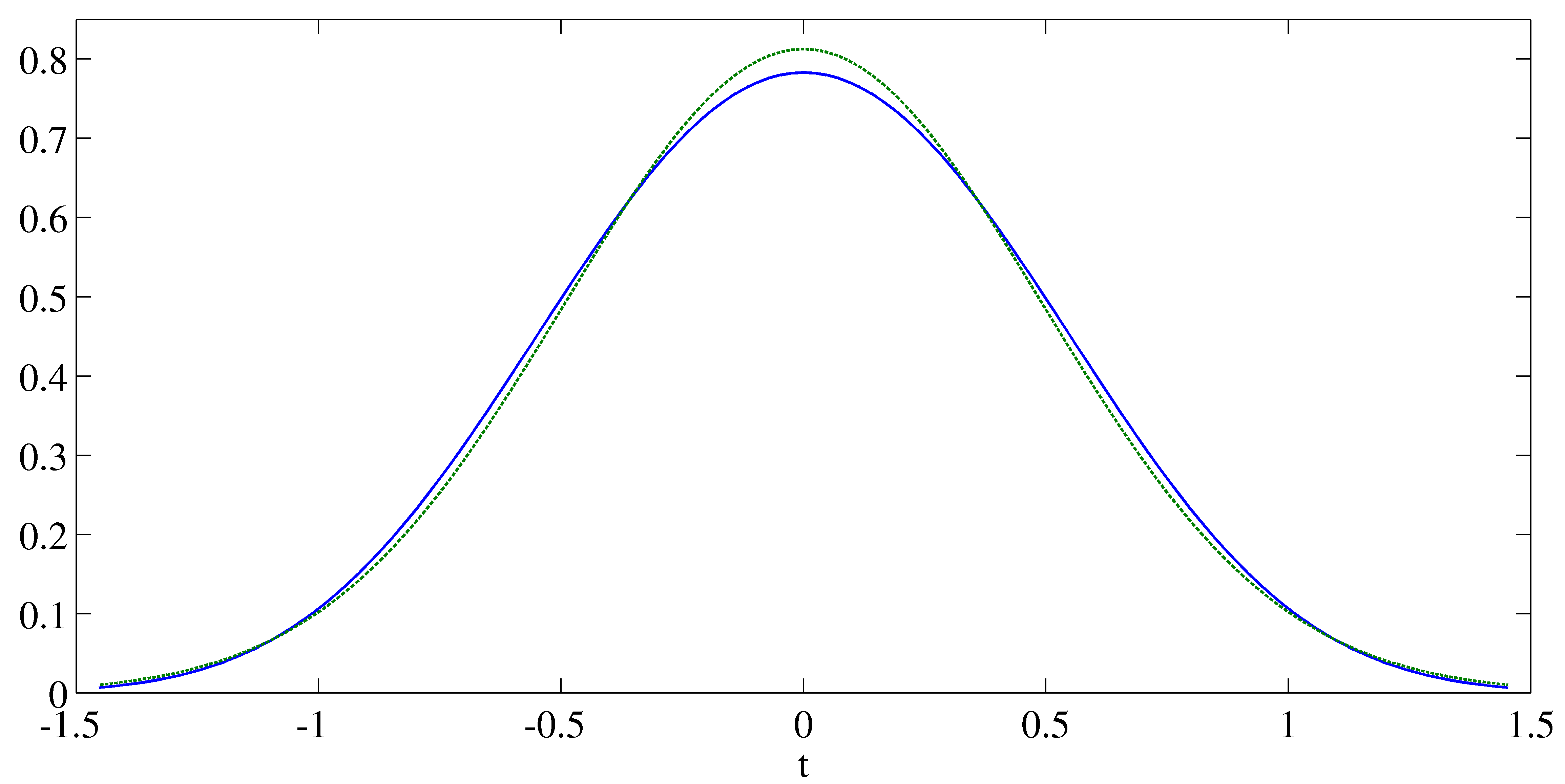
Figure 2. Plot of the density of $\mathcal{T}$ compared with a Gaussian density with the same variance 0.2409 (dashed line). The excess kurtosis $\mathbb{E}(\mathcal{T}^{4})/\mathbb{E}(\mathcal{T}^{2})^{2}-3$ is $-0.2374$.

One can readily check nevertheless that $f_{\rm end}(t)$ is symmetric in $t$. In [QR12] it is shown that the tails decay like $e^{-ct^{3}}$. Figure 1 shows a contour plot of the joint density of $\mathcal{M}$ and $\mathcal{T}$, while Figure 2 shows a plot of the marginal $\mathcal{T}$ density. The numerical computations of Fredholm determinants used to produce these plots are based on the numerical scheme and Matlab toolbox developed by F. Bornemann in [Bor10, Bor10a].

Although one only has the rigorous result in the case of geometric (or exponential) last passage percolation, the key point is that the polymer endpoint density $f_{\rm end}(t)$ is expected to be universal for directed polymers in random environment in $1+1$ dimensions, and even more broadly in the KPZ universality class, for example in particle models such as asymmetric attractive interacting particle systems (e.g. the asymmetric exclusion process), where second class particles play the role of polymer paths. And the analogous picture is expected to hold, as we now describe.

In the directed polymer models we consider a family $\big{\{}w(i,j)\}_{i\in\mathbb{Z}^{+},j\in\mathbb{Z}}$ of independent identically distributed random variables and the probability measure (polymer measure) ${\mathrm{\textbf{P}}}^{w}_{n,\beta}$ on the set $\Pi_{n}$ of one-dimensional nearest-neighbor random walks of length $n$ starting at $0$ given by

(1.13) $${\mathrm{\textbf{P}}}^{w}_{n,\beta}(\pi)=\frac{e^{\beta\sum_{i=0}^{n}w(i,\pi(i))}}{\sum_{\pi\in\Pi_{n}}e^{\beta\sum_{i=0}^{n}w(i,\pi(i))}},$$

where $\beta>0$ is the inverse temperature. The analogue of $\mathcal{T}_{n}$ in this context is $\pi(n)$, the random position of the endpoint. The last passage percolation case corresponds to $\beta=\infty$. The infinite temperature case $\beta=0$ is nothing but a free random walk. For $\beta<\infty$ the endpoint is random even given the random environment $\big{\{}w(i,j)\}_{i\in\mathbb{Z}^{+},j\in\mathbb{Z}}$. Still one expects in great generality, and for any $\beta>0$, to have

(1.14) $$cn^{-2/3}\pi(n)\xrightarrow{\rm distr}f_{\rm end}$$

for an appropriate $c$. The conjecture is that this holds whenever $E[w_{+}^{5}]<\infty$, and fails otherwise due to the appearance of special large values of $w$ which attract the polymer. However, few results are available at finite temperature. The first model for which any results were obtained (for the free energy) is the continuum random polymer (see below). There are now two other models, the semi-discrete model of O’Connell-Yor [OY01], and the log-Gamma polymer [Sep12, COSZ11], for which results about asymptotic fluctuations of the free energy are becoming available.

In the context of the continuum random polymer, we have continuous paths $x(s)$, $0<s<t$, starting at $0$ at time $0$, with quenched random energy

(1.15) $$\mathcal{H}(x(\cdot))=\int_{0}^{t}\{|\dot{x}(s)|^{2}-\xi(s,x(s))\}ds,$$

where $\xi$ is Gaussian space-time white noise, that is, $\langle\dot{\xi}(t,x),\dot{\xi}(s,y)\rangle=\delta(t-s)\delta(y-x)$. Through a mollification procedure [AKQ12] one can construct a probability measure $P^{\xi}_{t}$ on the space of continuous paths corresponding to the formal weights $e^{-\beta\mathcal{H}}$. It has finite dimensional distributions $P^{\xi}(x(t_{1})\in dx_{1},\ldots,x(t_{n})\in dx_{n},x(t)\in dx)$, $0<t_{1}<\dots<t_{n}<t$, given by

(1.16) $$\frac{Z(0,0,t_{1},x_{1})\cdots Z(t_{n-1},x_{n-1},t_{n},x_{n})Z(t_{n},x_{n},t,x)}{\int dy\,Z(0,0,t,y)}dx_{1}\cdots dx_{n}\,dx$$

where $Z(s,y,t,x)$ is the solution of the stochastic heat equation with multiplicative noise

$$\partial_{t}Z=\beta^{-1}\partial_{x}^{2}Z+\beta\xi Z$$

on $(s,t]$ with initial data $Z(s,y,s,x)=\delta(x-y)$. The temperature can be related to time as $t\sim\beta^{4}$, so through a time rescaling we can set $\beta=1$ without loss of generality.

In this setting the endpoint distribution is

(1.17) $$P^{\xi}_{t}(x(t)\in dx)=\frac{Z(0,0,t,x)}{\int dy\,Z(0,0,t,y)}dx.$$

Writing

(1.18) $$Z(0,0,t,x)=\tfrac{1}{\sqrt{4\pi t}}e^{-\tfrac{x^{2}}{4t}+(4t)^{1/3}A_{t}((4t)^{-2/3}x)+\tfrac{t}{24}}$$

the key prediction (see Conjecture 1.5 of [ACQ11]) is that, as $t\to\infty$, the crossover process $A_{t}$ converges to the Airy₂ process,

(1.19) $$A_{t}(x)\to\mathcal{A}_{2}(x).$$

This is proved in the sense of one dimensional marginals in [ACQ11, SS10], and a non-rigorous computation for multidimensional distributions was made in [PS11]. Calling $\tilde{x}=(4t)^{-2/3}x$ we can rewrite the exponent in (1.18) as $(4t)^{1/3}\{A_{t}(\tilde{x})-\tilde{x}^{2}\}+\frac{t}{24}$, from which we conclude that the endpoint of the polymer at time $t$ has approximately the distribution $(4t)^{2/3}\mathcal{T}$ for large $t$. The partition functions of discrete directed polymer models satisfy discrete versions of the stochastic heat equation, and analogous results are expected to hold in that setting as well.

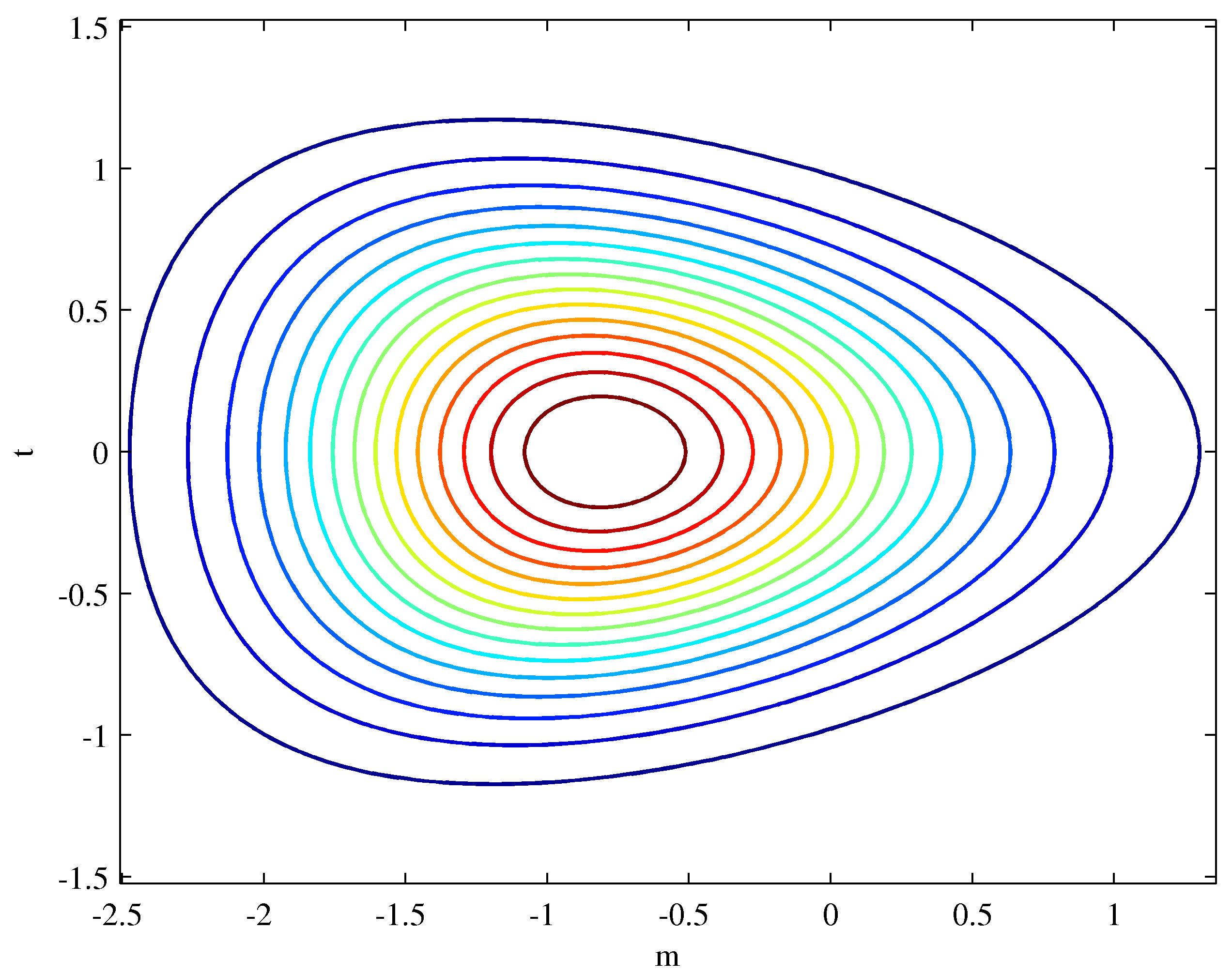
Figure 1. Contour plot of the joint density of $\mathcal{M}$ and $\mathcal{T}$.

The problem has attracted interested in the physics literature for quite some time (see for example [MP92, HHZ95]). Recently there has been a resurgence of interest. In particular, an alternate way to obtain the Airy₂ process is as a limit in large $N$ of the top path in a system of $N$ non-intersecting random walks, or Brownian motions, the so called vicious walkers [Fis84]. [SMCRF08], [Fei09] and [RS10, RS11] obtain various expressions for the joint distributions of $\mathcal{M}$ and $\mathcal{T}$ in such a system at finite $N$. [FMS11] obtain the $F_{\rm GOE}$ distribution from large $N$ asymptotics non-rigorously, and furthermore make connections between these problems and Yang-Mills theory. Unfortunately, the formulas obtained for $\mathcal{T}$ at finite $N$ have not been amenable to asymptotic analysis.

Acknowledgements

JQ and DR were supported by the Natural Science and Engineering Research Council of Canada, and DR was supported by a Fields-Ontario Postdoctoral Fellowship. GMF was supported by a postdoctoral position at the Fields Institute. The authors thank Ivan Corwin, Victor Dotsenko and Konstantine Khanin for interesting and helpful discussions, and Kurt Johansson for several references to the physics literature. They also thank Folkmar Bornemann for providing the Matlab toolbox on which numerical computations were based. This work was done during the Fields Institute program “Dynamics and Transport in Disordered Systems” and the authors would like to thank the Fields Institute for its hospitality. JQ would like in particular to acknowledge that the idea to work on this problem arose out of discussions with Victor Dotsenko during his visit to the Fields Institute.

2. Derivation of the formula

Let $(\mathcal{M}_{L},\mathcal{T}_{L})$ denote the maximum and the location of the maximum of $\mathcal{A}_{2}(t)-t^{2}$ restricted to $t\in[-L,L]$, and let $f_{L}$ be the joint density of $(\mathcal{M}_{L},\mathcal{T}_{L})$. We first note that, by results of I. Corwin and A. Hammond [CH11], the joint density $f(m,t)$ of $\mathcal{M},\mathcal{T}$ is well approximated by $f_{L}(m,t)$,

(2.1) $$f(t,m)=\lim_{L\to\infty}f_{L}(t,m).$$

By definition,

$$f_{L}(t,m)=\lim_{\delta\to 0}\lim_{\varepsilon\to 0}\frac{1}{\varepsilon\delta}\mathbb{P}\!\left(\mathcal{M}_{L}\in[m,m+\varepsilon],\,\mathcal{T}_{L}\in[t,t+\delta]\right),$$

provided that the limit exists. The main contribution in the above expression comes from paths entering the space-time box $[t,t+\delta]\times[m,m+\varepsilon]$ and staying below the level $m$ outside the time interval $[t,t+\delta]$. More precisely, if we denote by $\underline{D}_{\varepsilon,\delta}$ and $\overline{D}_{\varepsilon,\delta}$ the sets

(2.2) $$\underline{D}_{\varepsilon,\delta} =\Big{\{}\mathcal{A}_{2}(s)-s^{2}\leq m,\,\,\,s\in[t,t+\delta]^{\text{c}},\,\mathcal{A}_{2}(s)-s^{2}\leq m+\varepsilon,\,\,\,s\in[t,t+\delta],$$

$$\hskip 187.90244pt\mathcal{A}_{2}(s)-s^{2}\in[m,m+\varepsilon]\text{ for some }s\in[t,t+\delta]\Big{\}},$$

$$\@@ams@intertext{and}$$

$$\overline{D}_{\varepsilon,\delta} =\Big{\{}\mathcal{A}_{2}(s)-s^{2}\leq m+\varepsilon,\,\,\,s\in[-L,L],\,\mathcal{A}_{2}(s)-s^{2}\in[m,m+\varepsilon]\text{ for some }s\in[t,t+\delta]\Big{\}},$$

then

(2.3) $$\underline{D}_{\varepsilon,\delta}\subseteq\left\{\mathcal{M}_{L}\in[m,m+\varepsilon],\,\mathcal{T}_{L}\in[t,t+\delta]\right\}\subseteq\overline{D}_{\varepsilon,\delta}.$$

Letting $\underline{f}(t,m)=\lim_{\delta\to 0}\lim_{\varepsilon\to 0}\frac{1}{\varepsilon\delta}\mathbb{P}\big{(}\underline{D}_{\varepsilon,\delta}\big{)}$ and defining $\overline{f}(t,m)$ analogously (with $\overline{D}_{\varepsilon,\delta}$ instead of $\underline{D}_{\varepsilon,\delta}$) we deduce that $\underline{f}(t,m)\leq f(t,m)\leq\overline{f}(t,m)$. In what follows we will compute $\underline{f}(t,m)$. It will be clear from the argument that for $\overline{f}(t,m)$ we get the same limit, so we will only compute $\underline{f}(t,m)$. The conclusion is that

$$f_{L}(t,m)=\lim_{\delta\to 0}\lim_{\varepsilon\to 0}\frac{1}{\varepsilon\delta}\mathbb{P}\big{(}\underline{D}_{\varepsilon,\delta}\big{)}.$$

We rewrite this last equation as

(2.4) $$f_{L}(t,m)=\lim_{\delta\to 0}\lim_{\varepsilon\to 0}\frac{1}{\varepsilon\delta}\Big{[}\,\mathbb{P}\!\left(\mathcal{A}_{2}(s)\leq h_{\varepsilon,\delta}(s),\,s\in[-L,L]\right)-\mathbb{P}\!\left(\mathcal{A}_{2}(s)\leq h_{0,\delta}(s),\,s\in[-L,L]\right)\Big{]},$$

where

$$h_{\varepsilon,\delta}(s)=s^{2}+m+\varepsilon\mathbf{1}_{s\in[t,t+\delta]}.$$

Our method is based on precise computation of the two probabilities. We recall the formula in Theorem LABEL:g-thm:aiL of [CQR12] for the probability that $\mathcal{A}_{2}(t)\leq g(t)$ on a finite interval. Introduce the operator $\Theta^{g}_{[\ell,r]}$ which acts on $L^{2}(\mathbb{R})$ as follows: $\Theta^{g}_{[\ell,r]}f(\cdot)=u(r,\cdot)$, where $u(r,\cdot)$ is the solution at time $r$ of the boundary value problem

(2.5) $$\partial_{t}u+Hu =0\quad\text{for }x<g(t),~{}t\in(\ell,r)$$

$$u(\ell,x) =f(x)\mathbf{1}_{x<g(\ell)}$$

$$u(t,x) =0\quad\text{for }x\geq g(t)$$

for the Airy Hamiltonian,

$$H=-\partial_{x}^{2}+x.$$

In [CQR12] it is shown that this operator describes the height statistics of the Airy₂ process,

(2.6) $$\mathbb{P}\!\left(\mathcal{A}_{2}(t)\leq g(t)\text{ for }t\in[\ell,r]\right)=\det\!\left(I-K_{\operatorname{Ai}}+e^{-\ell H}K_{\operatorname{Ai}}\Theta^{g}_{[\ell,r]}e^{rH}K_{\operatorname{Ai}}\right),$$

where we have used the cyclic property of determinants as in (LABEL:g-eq:basiccyclic) in [CQR12]. We use (2.6) to rewrite (2.4) as

(2.7) $$f_{L}(t,m) =\lim_{\delta\to 0}\lim_{\varepsilon\to 0}\frac{1}{\varepsilon\delta}\left[\det\!\left(I-K_{\operatorname{Ai}}+e^{LH}K_{\operatorname{Ai}}\Theta^{h_{\varepsilon,\delta}}_{[-L,L]}e^{LH}K_{\operatorname{Ai}}\right)\right.$$

(2.8) $$\hskip 184.9429pt\left.-\det\!\left(I-K_{\operatorname{Ai}}+e^{LH}K_{\operatorname{Ai}}\Theta^{h_{0,\delta}}_{[-L,L]}e^{LH}K_{\operatorname{Ai}}\right)\right].$$

The limit in $\varepsilon$ becomes a derivative

(2.9) $$f_{L}(t,m) =\lim_{\delta\to 0}\frac{1}{\delta}\,\partial_{\beta}\!\left.\det\!\left(I-K_{\operatorname{Ai}}+e^{LH}K_{\operatorname{Ai}}\Theta^{h_{\beta,\delta}}_{[-L,L]}e^{LH}K_{\operatorname{Ai}}\right)\right|_{\beta=0},$$

which in turn gives a trace,

(2.10) $$f_{L}(t,m)=\det\!\left(I-K_{\operatorname{Ai}}+e^{LH}K_{\operatorname{Ai}}\Theta^{h_{0,\delta}}_{[-L,L]}e^{LH}K_{\operatorname{Ai}}\right)\\ \cdot\lim_{\delta\to 0}\frac{1}{\delta}\operatorname{tr}\!\left[(I-K_{\operatorname{Ai}}+e^{LH}K_{\operatorname{Ai}}\Theta^{h_{0,\delta}}_{[-L,L]}e^{LH}K_{\operatorname{Ai}})^{-1}e^{LH}K_{\operatorname{Ai}}\left[\partial_{\beta}\Theta^{h_{\beta,\delta}}_{[-L,L]}\right]_{\beta=0}e^{LH}K_{\operatorname{Ai}}\right]$$

(see Lemma A.2 and Remark A.3). Note that $h_{0,\delta}=g_{m}$, where $g_{m}$ is the parabolic barrier

(2.11) $$g_{m}(s)=s^{2}+m,$$

so in particular the determinant and the first factor inside the trace do not depend on $\delta$. From (LABEL:g-eq:omega) and Theorem LABEL:g-thm:goe from [CQR12] we have

(2.12) $$\lim_{L\to\infty}\left(I-K_{\operatorname{Ai}}+e^{LH}K_{\operatorname{Ai}}\Theta^{h_{0,\delta}}_{[-L,L]}e^{LH}K_{\operatorname{Ai}}\right)=I-A\bar{P}_{0}\hat{R}^{1}\bar{P}_{0}A^{*}$$

in trace norm, where $\bar{P}_{a}=I-P_{a}$ denotes the projection onto the interval $(-\infty,a]$,

(2.13) $$\hat{R}^{1}(\lambda,\tilde{\lambda})=2^{-1/3}\operatorname{Ai}(2^{-1/3}(2m-\lambda-\tilde{\lambda}),$$

and the Airy transform, $A$, acts on $f\in L^{2}(\mathbb{R})$ as

$$Af(x)=\int_{-\infty}^{\infty}dz\,\operatorname{Ai}(x-z)f(z).$$

In particular, (LABEL:g-eq:goe) in [CQR12] implies that

(2.14) $$\lim_{L\to\infty}\det\!\left(I-K_{\operatorname{Ai}}+e^{LH}K_{\operatorname{Ai}}\Theta^{h_{0,\delta}}_{[-L,L]}e^{LH}K_{\operatorname{Ai}}\right)=F_{\mathrm{GOE}}(4^{1/3}m).$$

The next step is to compute $\partial_{\beta}\Theta^{h_{\beta,\delta}}_{[-L,L]}\!\mid_{\beta=0}$. Recalling that $h_{0,\delta}(s)=g_{m}(s)=s^{2}+m$ and also $h_{\varepsilon,\delta}(s)=g_{m+\varepsilon}(s)$ for $s\in[t,t+\delta]$ we have, by the semigroup property,

$$\Theta^{h_{\varepsilon,\delta}}_{[-L,L]}-\Theta^{h_{0,\delta}}_{[-L,L]}=\Theta^{g_{m}}_{[-L,t]}\left[\Theta^{g_{m+\varepsilon}}_{[t,t+\delta]}-\Theta^{g_{m}}_{[t,t+\delta]}\right]\Theta^{g_{m}}_{[t+\delta,L]}.$$

We now use Theorem LABEL:g-thm:thetaLgen of [CQR12] and a minor variation of (LABEL:g-eq:thetaL) in [CQR12] to obtain that $\Theta^{g_{m}}_{[\ell,r]}$ has explicit integral kernel

(2.15) $$\Theta^{g_{m}}_{[\ell,r]}(x,y)=\frac{e^{\ell x-ry+(r^{3}-\ell^{3})/3}}{\sqrt{4\pi(r-\ell)}}\left[e^{-\frac{(x-\ell^{2}-y+r^{2})^{2}}{4(r-\ell)}}-e^{-\frac{(x-\ell^{2}+y-r^{2}-2m)^{2}}{4(r-\ell)}}\right]\mathbf{1}_{x\leq m+\ell^{2}}\mathbf{1}_{y\leq m+r^{2}}.$$

For convenience we introduce the kernels $\vartheta_{1}(x,z)=e^{tz}\widetilde{\Theta}^{h_{0,0}}_{[-L,t]}(x,z)\mathbf{1}_{x\leq m+L^{2}}$ and $\vartheta_{2}(\tilde{z},y)=e^{-t\tilde{z}}\widetilde{\Theta}^{h_{0,0}}_{[t+\delta,L]}(\tilde{z},y)\mathbf{1}_{y\leq m+L^{2}}$, where $\widetilde{\Theta}^{h_{0,0}}_{[\ell,r]}$ is defined as in (2.15) but with the indicator functions replaced by 1. Let

(2.16) $$\Lambda^{\varepsilon,\delta}_{L}(x,y)=\frac{1}{\sqrt{4\pi\delta}}e^{[(t+\delta)^{3}-t^{3}]/3}\int_{-\infty}^{m+t^{2}}dz\int_{-\infty}^{m+(t+\delta)^{2}}\!\!d\tilde{z}\,\vartheta_{1}(x,z)\\ \cdot\left[e^{-(z-t^{2}+\tilde{z}-(t+\delta)^{2}-2m)^{2}/(4\delta)}-e^{-(z-t^{2}+\tilde{z}-(t+\delta)^{2}-2m-2\varepsilon)^{2}/(4\delta)}\right]\!\vartheta_{2}(\tilde{z},y),$$

which corresponds to $\Theta^{h_{\varepsilon,\delta}}_{[-L,L]}-\Theta^{h_{0,\delta}}_{[-L,L]}$ but without shifting $m$ by $\varepsilon$ in the indicator functions in (2.15) for the first operator in this difference. We will show in Lemma A.4 that

(2.17) $$\lim_{\varepsilon\to 0}\frac{1}{\varepsilon}\left[\left(\Theta^{h_{\varepsilon,\delta}}_{[-L,L]}-\Theta^{h_{0,\delta}}_{[-L,L]}\right)-\Lambda^{\varepsilon,\delta}_{L}\right]=0$$

in Hilbert-Schmidt norm. On the other hand, performing in (2.16) first the change of variables $z\mapsto z+m+t^{2}$, $\tilde{z}\mapsto\tilde{z}+m+(t+\delta)^{2}$, then a scaling of $z$ and $\tilde{z}$ by $\sqrt{\delta}$, and then the change of variables $-u=z+\tilde{z}$, $-v=z-\tilde{z}$, we get

(2.18) $$\Lambda^{\varepsilon,\delta}_{L}(x,y)=\frac{e^{[(t+\delta)^{3}-t^{3}]/3}}{4\sqrt{\pi}}\int^{\infty}_{0}du\int^{u}_{-u}dv\,\vartheta_{1}(x,-\sqrt{\delta}(u+v)/2+m+t^{2})\\ \sqrt{\delta}\left[e^{-u^{2}/4}-e^{-(u+2\varepsilon/\sqrt{\delta})^{2}/4}\right]\vartheta_{2}(\sqrt{\delta}(v-u)/2+m+(t+\delta)^{2},y),$$

From this form and (2.17) it is straightforward to see that

(2.19) $$\lim_{\varepsilon\to 0}\frac{1}{\varepsilon}\bigg{[}\Theta^{h_{\varepsilon,\delta}}_{[-L,L]}-\Theta^{h_{0,\delta}}_{[-L,L]}\bigg{]}(x,y)=\lim_{\varepsilon\to 0}\frac{1}{\varepsilon}\Lambda^{\varepsilon,\delta}_{L}(x,y)\\ =\frac{1}{4\sqrt{\pi}}\int^{\infty}_{0}du\int^{u}_{-u}dv\,u\,e^{-u^{2}/4}\,\vartheta_{1}(x,-\sqrt{\delta}(u+v)/2+m+t^{2})\vartheta_{2}(\sqrt{\delta}(v-u)/2+m+(t+\delta)^{2},y).$$

The limit holds in Hilbert-Schmidt norm, as will be shown in Lemma A.4. Now we take the limit in $\delta$ and obtain

(2.20) $$\lim_{\delta\to 0}\frac{1}{\delta}\left[\partial_{\beta}\Theta^{h_{\beta,\delta}}_{[-L,L]}\right]_{\beta=0}(x,y)=\partial_{w}\vartheta_{1}(x,w)|_{w=m+t^{2}}\,\partial_{w}\vartheta_{2}(w,y)|_{w=m+t^{2}},$$

again in Hilbert-Schmidt norm, which will be checked in Lemma A.4. Referring back to (2.10) we have now shown that

(2.21) $$\lim_{\delta\to 0}\frac{1}{\delta}e^{LH}K_{\operatorname{Ai}}\left[\partial_{\beta}\Theta^{h_{\beta,\delta}}_{[-L,L]}\right]_{\beta=0}e^{LH}K_{\operatorname{Ai}}=\widetilde{\Psi}_{L},$$

where $\widetilde{\Psi}_{L}$ has kernel

$$\widetilde{\Psi}_{L}(x,y)=\widetilde{\Psi}^{1}_{L}(x)\widetilde{\Psi}^{2}_{L}(y)$$

with

(2.22) $$\widetilde{\Psi}^{1}_{L}(x) =\left.\partial_{w}\big{(}e^{LH}K_{\operatorname{Ai}}\widetilde{\Theta}^{g_{m}}_{[-L,t]}M_{t}(x,w)\big{)}\right|_{w=m+t^{2}},$$

$$\widetilde{\Psi}^{2}_{L}(y) =\left.\partial_{w}\big{(}M_{-t}\widetilde{\Theta}^{g_{m}}_{[t,L]}e^{LH}K_{\operatorname{Ai}}(w,y)\big{)}\right|_{w=m+t^{2}},$$

and $M_{t}$ is the multiplication operator given by $M_{t}f(x)=e^{tx}f(x)$.

Putting (2.1), (2.10), (2.14) and (2.21) together and using Lemma A.1(a) we have

(2.23) $$f(t,m)=\lim_{L\to\infty}\operatorname{tr}\!\left[(I-K_{\operatorname{Ai}}+e^{LH}K_{\operatorname{Ai}}\Theta^{g_{m}}_{[-L,L]}e^{LH}K_{\operatorname{Ai}})^{-1}\widetilde{\Psi}_{L}\right]F_{\mathrm{GOE}}(4^{1/3}m).$$

We now have to compute the limit of the trace. We begin by using (2.15) to compute

$$\varphi(z):=\partial_{w}\big{(}\widetilde{\Theta}^{g_{0}}_{[-L,t]}M_{t}(z,w)\big{)}\Big{|}_{w=m+t^{2}}=\frac{e^{-Lz+L^{3}/3+t^{3}/3}}{2\sqrt{\pi}(L+t)^{3/2}}(z-m-L^{2})\,e^{-(z-m-L^{2})^{2}/4(L+t)}.$$

Note how the derivative of the two terms inside the bracket in (2.15) evaluated at $w=m+t^{2}$ are equal. From (2.22) we get

(2.24) $$\widetilde{\Psi}^{1}_{L}(x)=e^{LH}K_{\operatorname{Ai}}\bar{P}_{m+L^{2}}\,\varphi(x)=e^{LH}K_{\operatorname{Ai}}\,\varphi(x)-e^{LH}K_{\operatorname{Ai}}P_{m+L^{2}}\,\varphi(x),$$

In Appendix A we will show that

(2.25) $$\lim_{L\to\infty}\left\|e^{LH}K_{\operatorname{Ai}}P_{m+L^{2}}\,\varphi\right\|_{L^{2}(\mathbb{R})}=0.$$

Now we compute $e^{LH}K_{\operatorname{Ai}}\varphi$. We write it as

(2.26) $$e^{LH}K_{\operatorname{Ai}}\,\varphi(x)=\int_{-\infty}^{0}d\lambda\,e^{\lambda L}\operatorname{Ai}(x-\lambda)\int_{-\infty}^{\infty}dz\,\operatorname{Ai}(z-\lambda)\,\varphi(z).$$

To compute the $z$ integral, which we denote by $I(\lambda)$, we use the contour integral representation of the Airy function given by

(2.27) $$\operatorname{Ai}(x)=\frac{1}{2\pi{\rm i}}\int_{\Gamma}du\,e^{u^{3}/3-ux},$$

with $\Gamma=\{c+{\rm i}s\!:s\in\mathbb{R}\}$ and $c$ any positive real number, to write

$$I(\lambda)=\frac{1}{2\pi{\rm i}}\int_{\Gamma}du\int_{-\infty}^{\infty}dz\,e^{u^{3}/3-u(z+m+L^{2}-\lambda)}\frac{e^{-L(z+m+L^{2})+L^{3}/3+t^{3}/3}}{2\sqrt{\pi}(L+t)^{3/2}}\,e^{-z^{2}/4(L+t)}\,z,$$

where we have shifted the variable $z$ by $m+L^{2}$. Note that the integral in $z$ is of the form $\int_{-\infty}^{\infty}dz\,e^{-a_{1}z^{2}-a_{2}z-a_{3}}z$, which corresponds to computing the mean of a certain Gaussian random variable. Performing the integration we get

$$I(\lambda)=-\frac{2}{2\pi{\rm i}}\int_{\Gamma}du\,e^{u^{3}/3+(L+t)u^{2}+(L^{2}+2Lt-m+\lambda)u-Lm+L^{3}/3+L^{2}t+t^{3}/3}(L+u).$$

Introducing the change of variables $u=v-L-t$ we get

$$I(\lambda)=-\frac{2}{2\pi{\rm i}}\,e^{mt+t^{3}-(L+t)\lambda}\int_{\Gamma^{\prime}}dv\,e^{v^{3}/3-(m+t^{2}-\lambda)v}(v-t),$$

where $\Gamma^{\prime}$ corresponds to a shift of $\Gamma$ along the real axis. Using (2.27) we deduce that

$$I(\lambda)=2\,e^{mt+t^{3}-(L+t)\lambda}\Big{[}\!\operatorname{Ai}^{\prime}(m+t^{2}-\lambda)+t\operatorname{Ai}(m+t^{2}-\lambda)\Big{]}.$$

Therefore

$$e^{LH}K_{\operatorname{Ai}}\varphi(x)=2\int_{-\infty}^{0}d\lambda\,e^{t^{3}+(m-\lambda)t}\operatorname{Ai}(x-\lambda)\Big{[}\operatorname{Ai}^{\prime}(m+t^{2}-\lambda)+t\operatorname{Ai}(m+t^{2}-\lambda)\Big{]}.$$

We will rewrite this identity as

$$e^{LH}K_{\operatorname{Ai}}\varphi(x)=A\bar{P}_{0}\widetilde{\psi}_{t,m}(x),$$

where

(2.28) $$\widetilde{\psi}_{t,m}(x)=2e^{t^{3}+(m-x)t}\bigg{[}\operatorname{Ai}^{\prime}(m+t^{2}-x)+t\operatorname{Ai}(m+t^{2}-x)\bigg{]}.$$

Remarkably, the result does not depend on $L$. Note that $A\bar{P}_{0}\widetilde{\psi}_{t,m}\in L^{2}(\mathbb{R})$, which can be checked using the Plancherel formula for the Airy transform

(2.29) $$\int(Af)^{2}=\int\!f^{2}$$

and the fact that $|\!\operatorname{Ai}(u)|\vee|\!\operatorname{Ai}^{\prime}(u)|\leq Ce^{-\frac{2}{3}u^{3/2}}$ for some $C>0$ and all $u>0$ (see (10.4.59-60) in [AS64]).

Now we look at $\widetilde{\Psi}^{2}_{L}(y)$. By the time symmetry and time homogeneity of the heat kernel it is clear that $\partial_{w}\big{(}M_{-t}\widetilde{\Theta}^{g_{m}}_{[t,L]}(w,\cdot)\big{)}(y)\big{|}_{w=m+t^{2}}$ can be obtained from the above calculation by starting at $y$ and running backwards in time from $L$ to $t$. Observe that the length of this time interval is $L-t$, whereas the one in the above calculation had length $L+t$. Moreover, here we are multiplying the boundary value operator by $M_{-t}$, whereas before we multiplied by $M_{t}$. It is not difficult then to see that the answer for the second factor should be the same as for the first one, only with $x$ replaced by $y$ and $t$ by $-t$. From this, (2.22) and (2.25) we get that

(2.30) $$\widetilde{\Psi}_{L}(x,y)\xrightarrow[L\to\infty]{}\widetilde{\Psi}(x,y):=A\bar{P}_{0}\widetilde{\psi}_{t,m}(x)A\bar{P}_{0}\widetilde{\psi}_{-t,m}(y)$$

in Hilbert-Schmidt sense, and thus from (2.12) and Lemma A.1(b) we have that

(2.31) $$(I-K_{\operatorname{Ai}}+e^{LH}K_{\operatorname{Ai}}\Theta^{h_{0,\delta}}_{[-L,L]}e^{LH}K_{\operatorname{Ai}})^{-1}\widetilde{\Psi}_{L}\xrightarrow[L\to\infty]{}(I-A\bar{P}_{0}\hat{R}^{1}\bar{P}_{0}A^{*})^{-1}\widetilde{\Psi}$$

in trace norm (the product converges in trace norm thanks to Lemma LABEL:g-lem:fredholm of [CQR12]). Therefore by Lemma A.1(a),

(2.32) $$\lim_{L\to\infty}\operatorname{tr}\!\Big{[}(I-K_{\operatorname{Ai}}+e^{LH}K_{\operatorname{Ai}}\Theta^{h_{0,\delta}}_{[-L,L]}e^{LH}K_{\operatorname{Ai}})^{-1}\widetilde{\Psi}_{L}\Big{]}\\ =\operatorname{tr}\!\left[(I-A\bar{P}_{0}\hat{R}^{1}\bar{P}_{0}A^{*})^{-1}\widetilde{\Psi}\right]=\left\langle(I-A\bar{P}_{0}\hat{R}^{1}\bar{P}_{0}A^{*})^{-1}A\bar{P}_{0}\widetilde{\psi}_{t,m},A\bar{P}_{0}\widetilde{\psi}_{-t,m}\right\rangle_{L^{2}(\mathbb{R})},$$

where $\langle\cdot,\cdot\rangle_{\mathcal{H}}$ denotes inner product in the Hilbert space $\mathcal{H}$ (with $\mathcal{H}=L^{2}(\mathbb{R})$ if the subscript is omitted).

It only remains to simplify the expression. We use the reflection operator $\sigma f(x)=f(-x)$. Because $(A\sigma)^{-1}=A\sigma$, $\sigma^{2}=I$ and $A^{*}=\sigma A\sigma$, we have

(2.33) $$\left\langle(I-A\bar{P}_{0}\hat{R}^{1}\bar{P}_{0}A^{*})^{-1}A\bar{P}_{0}\widetilde{\psi}_{t,m},A\bar{P}_{0}\widetilde{\psi}_{-t,m}\right\rangle=\left\langle A\sigma(I-\sigma\bar{P}_{0}\hat{R}^{1}\bar{P}_{0}\sigma)^{-1}\sigma\bar{P}_{0}\widetilde{\psi}_{t,m},A\bar{P}_{0}\widetilde{\psi}_{-t,m}\right\rangle.$$

Since $(A\sigma)^{*}=A\sigma$ and $A\sigma A=\sigma$, this last term can be rewritten as

(2.34) $$\left\langle(I-\sigma\bar{P}_{0}\hat{R}^{1}\bar{P}_{0}\sigma)^{-1}\sigma\bar{P}_{0}\widetilde{\psi}_{t,m},(A\sigma)^{*}A\bar{P}_{0}\widetilde{\psi}_{-t,m}\right\rangle =\left\langle(I-\sigma\bar{P}_{0}\hat{R}^{1}\bar{P}_{0}\sigma)^{-1}\sigma\bar{P}_{0}\widetilde{\psi}_{t,m},\sigma\bar{P}_{0}\widetilde{\psi}_{-t,m}\right\rangle$$

$$=\left\langle(I-P_{0}\sigma\hat{R}^{1}\sigma P_{0})^{-1}\sigma\widetilde{\psi}_{t,m},\sigma\widetilde{\psi}_{-t,m}\right\rangle_{L^{2}([0,\infty))},$$

where in the second equality we used the trivial fact that $P_{0}\sigma=\sigma\bar{P}_{0}$ and $\sigma P_{0}=\bar{P}_{0}\sigma$. Observing that $\sigma\widetilde{\psi}_{t,m}(x)=e^{t^{3}+mt}\psi_{t,m}(x)$, where $\psi_{t,m}$ was defined in (1.9), we deduce that

(2.35) $$\left\langle(I-A\bar{P}_{0}\hat{R}^{1}\bar{P}_{0}A^{*})^{-1}A\bar{P}_{0}\widetilde{\psi}_{t,m},A\bar{P}_{0}\widetilde{\psi}_{-t,m}\right\rangle_{L^{2}(\mathbb{R})}=\left\langle(I-P_{0}\sigma\hat{R}^{1}\sigma P_{0})^{-1}\psi_{t,m},\psi_{-t,m}\right\rangle_{L^{2}([0,\infty))}.$$

Now we use the scaling operator $Sf(x)=f(2^{1/3}x)$. One can check easily that $S^{-1}=2^{1/3}S^{*}$ and that $P_{0}$ commutes with $S$ and $S^{-1}$. Since $\sigma\hat{R}^{1}\sigma(x,y)=2^{-1/3}\operatorname{Ai}(2^{-1/3}(x+y)+4^{1/3}m)$, we also have

$$S\sigma\hat{R}^{1}\sigma S^{-1}=B_{4^{1/3}m},$$

where this last kernel was defined in (1.6). Thus writing $\tilde{m}=2^{-1/3}m$ we get

(2.36) $$\Big{\langle}(I-P_{0}\sigma\hat{R}^{1}\sigma P_{0})^{-1}\psi_{t,m},\psi_{-t,m}\Big{\rangle}_{L^{2}([0,\infty))} =\left\langle(I-S^{-1}P_{0}B_{2\tilde{m}}P_{0}S)^{-1}\psi_{t,m},\psi_{-t,m}\right\rangle_{L^{2}([0,\infty))}$$

(2.37) $$=\left\langle S^{-1}(I-P_{0}B_{2\tilde{m}}P_{0})^{-1}S\psi_{t,m},\psi_{-t,m}\right\rangle_{L^{2}([0,\infty))}$$

(2.38) $$=2^{1/3}\left\langle(I-P_{0}B_{2\tilde{m}}P_{0})^{-1}S\psi_{t,m},S\psi_{-t,m}\right\rangle_{L^{2}([0,\infty))},$$

which is equal to $2^{1/3}\gamma(t,4^{1/3}m)$. This gives our first formula for $f(t,m)$ in (1.11). Now observe that $\gamma(t,4^{1/3}m)$ equals the trace of the operator $(I-P_{0}B_{4^{1/3}m}P_{0})^{-1}P_{0}\Psi_{t,m}P_{0}$ and that $\Psi_{t,m}$ is a rank one operator. The second equality in (1.11) now follows that from the general fact that for two operators $A$ and $B$ such that $B$ is rank one, one has $\det(I-A+B)=\det(I-A)\big{[}1+\operatorname{tr}\big{(}(I-A)^{-1}B\big{)}\big{]}$.

3. $\mathcal{M}$ marginal and uniqueness of the maximizer

As we mentioned in the introduction, [CH11] showed that the maximum of $\mathcal{A}_{2}(t)-t^{2}$ is attained at a unique point $t\in\mathbb{R}$, providing a proof of a conjecture by K. Johansson (Conjecture 1.5 in [Joh03]). We used their result in Section 2 to write formulas for $f(t,m)$ in terms of certain events concerning the Airy₂ process.

Alternatively, one can turn the reasoning around and use our formula to give a different proof of Johansson’s conjecture. If we do not assume the uniqueness of the maximizer, then the derivation in Section 2 leads to a density $f(t,m)$ for the event that there is a maximizer at $t$ (and height $m$). Therefore the uniqueness of the maximizer is equivalent to

(3.1) $$\int_{\mathbb{R}^{2}}dt\,dm\,f(t,m)=1.$$

This, in turn, is a direct consequence of the following

Proposition 3.1.

For any $m\in\mathbb{R}$,

$$\int_{-\infty}^{\infty}dt\,f(t,m)=\frac{d}{dm}F_{\rm GOE}(4^{1/3}m).$$

Proof.

From the formula (1.11) for $f(t,m)$ we see that we need to compute

$$\Psi_{m}(x,y)=\int_{-\infty}^{\infty}dt\,\psi_{-t,m}(\tilde{x})\psi_{t,m}(\tilde{y}),$$

where $\tilde{x}=2^{1/3}x$ and $\tilde{y}=2^{1/3}y$. Let $\Gamma_{a}=\{a+{\rm i}s\!:s\in\mathbb{R}\}$. Then fixing $a>0$ and using (2.27) we have

$$\Psi_{m}(x,y)=\frac{4}{(4\pi{\rm i})^{2}}\int_{\Gamma_{2a}\times\Gamma_{a}}du\,dv\int_{-\infty}^{\infty}dt\,(u-t)(v+t)e^{u^{3}/3+v^{3}/3-u({\tilde{x}}+m+t^{2})-v({\tilde{y}}+m+t^{2})+t({\tilde{x}}-{\tilde{y}})}.$$

The $t$ integral is just a Gaussian integral and gives

$$\Psi_{m}(x,y)=\frac{\sqrt{\pi}}{(4\pi{\rm i})^{2}}\int_{\Gamma_{2a}\times\Gamma_{a}}du\,dv\,(u+v)^{-5/2}p_{{\tilde{x}},{\tilde{y}}}(u,v)e^{q_{{\tilde{x}},{\tilde{y}}}(u,v)},$$

where

(3.2) $$p_{{\tilde{x}},{\tilde{y}}}(u,v) =4u^{3}v+4uv^{3}+8u^{2}v^{2}-2(u+v)+2(u^{2}-v^{2})({\tilde{x}}-{\tilde{y}})-({\tilde{x}}-{\tilde{y}})^{2}$$

and

(3.3) $$q_{{\tilde{x}},{\tilde{y}}}(u,v) =\frac{\frac{1}{3}(u^{4}+v^{4}+u^{3}v+uv^{3})-m(u+v)^{2}-u^{2}{\tilde{x}}-v^{2}{\tilde{y}}+\frac{1}{4}({\tilde{x}}-{\tilde{y}})^{2}-uv({\tilde{x}}+{\tilde{y}})}{u+v}.$$

Introducing the change of variables $z=u+v$, $w=u-v$, we get

$$\Psi_{m}(x,y)=\frac{-\sqrt{\pi}}{(4\pi{\rm i})^{2}}\frac{1}{2}\int_{\Gamma_{3a}}dz\int_{\Gamma_{a}}dw\,z^{-5/2}\tilde{p}_{{\tilde{x}},{\tilde{y}}}(z,w)e^{\tilde{q}_{{\tilde{x}},{\tilde{y}}}(z,w)},$$

where

(3.4) $$\tilde{p}_{{\tilde{x}},{\tilde{y}}}(z,w) =-w^{2}z^{2}+2wz({\tilde{x}}-{\tilde{y}})-({\tilde{x}}-{\tilde{y}})^{2}-2z+z^{4}$$

and

(3.5) $$\tilde{q}_{{\tilde{x}},{\tilde{y}}}(z,w) =\frac{w^{2}z^{2}-2wz({\tilde{x}}-{\tilde{y}})+({\tilde{x}}-{\tilde{y}})^{2}-2({\tilde{x}}+{\tilde{y}}+2m)z^{2}+\frac{1}{3}z^{4}}{4z}.$$

Changing variables $w\mapsto iw$, the $w$ integral is another Gaussian integral and we get

(3.6) $$\Psi_{m}(x,y) =\frac{1}{4\pi{\rm i}}\int_{\Gamma_{3a}}dz\,z\,e^{z^{3}/12-z({\tilde{x}}+{\tilde{y}}+2m)/2}=\frac{4^{2/3}}{4\pi{\rm i}}\int_{\Gamma_{4^{-1/3}3a}}dz\,z\,e^{z^{3}/3-2^{-1/3}z({\tilde{x}}+{\tilde{y}}+2\tilde{m})}$$

(3.7) $$=-2^{1/3}\operatorname{Ai}^{\prime}\!\big{(}x+y+4^{1/3}m)\big{)}=-2^{-1/3}\partial_{m}B_{4^{1/3}m}(x,y),$$

where we have used (2.27). Using this in the definition of $\gamma(t,m)$ we deduce that

$$\int_{-\infty}^{\infty}dt\,\gamma(t,m)=-2^{1/3}\operatorname{tr}\!\left[\left(I-P_{0}B_{m}P_{0}\right)^{-1}\Psi_{m}\right]=-\operatorname{tr}\!\left[\left(I-P_{0}B_{m}P_{0}\right)^{-1}\partial_{m}B_{m}\right].$$

Consequently we get from (1.11) and (1.7) that

$$\int_{-\infty}^{\infty}dt\,f(t,m)=-\operatorname{tr}\!\left[\left(I-P_{0}B_{m}P_{0}\right)^{-1}\partial_{m}B_{m}\right]\det\!\big{(}I-P_{0}B_{m}P_{0}\big{)}=\frac{d}{dm}\det\!\big{(}I-P_{0}B_{m}P_{0}\big{)},$$

where the last inequality follows from Lemma A.2. The result now follows from (1.7). ∎

Appendix A Technical estimates

Section LABEL:g-sec:aiL of [CQR12] contains a short review of some general facts about trace class and Hilbert-Schmidt operators and Fredholm determinants. In Section 2 of the present article we used some additional facts, which we state next. Here $\mathcal{H}$ will denote a separable Hilbert space and $\mathcal{B}_{1}(\mathcal{H})$ will denote the space of trace class operators in $\mathcal{H}$, which is endowed with the trace norm (see Section LABEL:g-sec:aiL of [CQR12] for a short discussion or [Sim05] for a complete treatment).

Lemma A.1.

Assume $\big{\{}\!A(v)\big{\}}_{v\geq 0}$ is a family of operators converging as $v\to\infty$ in $\mathcal{B}_{1}(\mathcal{H})$ to some operator $A\in\mathcal{B}_{1}(\mathcal{H})$. Then:

1. $\displaystyle\operatorname{tr}(A(v))\xrightarrow[v\to\infty]{}\operatorname{tr}(A)$.

2. If $I-A(v)$ is invertible for all large enough $v$ and $I-A$ is also invertible, then

   $$(I-A(v))^{-1}\xrightarrow[v\to\infty]{}(I-A)^{-1}\quad\text{in }\mathcal{B}_{1}(\mathcal{H}).$$

This result comes from Theorem 3.1 and Corollary 5.2 in [Sim05]. Using (5.1) from [Sim05] one can also easily show the following (see also the corollary just cited):

Lemma A.2.

Assume $\big{\{}\!A(\beta)\big{\}}_{\beta\in[0,1)}$ is a family of operators in $\mathcal{B}_{1}(\mathcal{H})$ such that there is an operator $\partial_{\beta}A(0)$ satisfying

$$\frac{1}{\beta}\left[A(\beta)-A(0)\right]\xrightarrow[\beta\to 0]{}\partial_{\beta}A(0)\quad\text{in }\mathcal{B}_{1}(\mathcal{H}).$$

Then the map $\beta\longmapsto\det\!\big{(}I+A(\beta)\big{)}$ is differentiable at 0 and

$$\partial_{\beta}\det\!\big{(}I+A(\beta)\big{)}\Big{|}_{\beta=0}=\operatorname{tr}\!\left[(I+A(0))^{-1}\partial_{\beta}A(0)\right]\det\!\big{(}I+A(0)\big{)}.$$

Remark A.3.

Note that the last two lemmas assume convergence in trace norm as the hypothesis. Throughout Section 2 (see (2.10), (2.19) and (2.20)) we used these results for operators of the form $e^{LH}K_{\operatorname{Ai}}\Phi_{\eta}e^{LH}K_{\operatorname{Ai}}$, where $\eta$ is some parameter and we know that $\Phi_{\eta}$ converges in Hilbert-Schmidt norm to some limit $\Phi$. As we will see in Lemma A.4, the convergence is in fact a bit stronger, and using this we can justify the application of the lemmas in Section 2. To see why, note that if we let $\varphi(x)=1+x^{2}$ and define the multiplication operator $Mf(x)=\varphi(x)f(x)$ then by Lemma LABEL:g-lem:fredholm of [CQR12] we have

(A.1) $$\|e^{LH}K_{\operatorname{Ai}}(\Phi_{\eta}-\Phi)e^{LH}K_{\operatorname{Ai}}\|_{1}\leq\|e^{LH}K_{\operatorname{Ai}}\|_{\rm op}\|(\Phi_{\eta}-\Phi)M\|_{2}\|M^{-1}e^{LH}K_{\operatorname{Ai}}\|_{2}.$$

By (2.26) we have, for $f\in L^{2}(\mathbb{R})$,

(A.2) $$\|e^{LH/2}K_{\operatorname{Ai}}f\|_{2}^{2} =\int_{\mathbb{R}^{3}}dx\,dy\,d\tilde{y}\int_{(-\infty,0]^{2}}d\lambda\,d\tilde{\lambda}\,e^{(\lambda+\tilde{\lambda})L/2}\operatorname{Ai}(x-\lambda)\operatorname{Ai}(y-\lambda)f(y)$$

(A.3) $$\hskip 216.81pt\cdot\operatorname{Ai}(x-\tilde{\lambda})\operatorname{Ai}(\tilde{y}-\tilde{\lambda})f(\tilde{y})$$

(A.4) $$=\int_{\mathbb{R}^{2}}dy\,d\tilde{y}\int_{(-\infty,0]^{2}}d\lambda\,d\tilde{\lambda}\,e^{(\lambda+\tilde{\lambda})L/2}\operatorname{Ai}(y-\lambda)f(y)\operatorname{Ai}(\tilde{y}-\tilde{\lambda})f(\tilde{y})\delta_{\lambda=\tilde{\lambda}}$$

(A.5) $$=\int_{-\infty}^{0}d\lambda\,e^{\lambda L}Af(\lambda)^{2}.$$

Using (2.29) we deduce that $\|A\|_{\rm op}=\|A^{*}\|_{\rm op}=1$, and then

(A.6) $$\|e^{LH/2}K_{\operatorname{Ai}}\|_{\rm op}\leq 1.$$

The third norm in (A.1) is also finite, thanks to (LABEL:g-eq:sndHS) in [CQR12], and we are going to prove below the convergence $\|(\Phi_{\eta}-\Phi)M\|_{2}\to 0$ in each relevant case.

The next result provides the missing estimates in the proof of (2.23).

Lemma A.4.

For each fixed $\delta,L>0$, the convergences in (2.17), (2.19) and (2.20) hold in Hilbert-Schmidt norm. Moreover, if we let $\varphi(x)=1+x^{2}$ and define the multiplication operator $Mf(x)=\varphi(x)f(x)$, then the three convergences above still hold if we multiply each operator on the right by $M$.

Proof.

The second equality in (2.19) one follows from the dominated convergence theorem and the estimate

(A.7) $$\left|\frac{\sqrt{\delta}}{\varepsilon}\left[e^{-u^{2}/4}-e^{-(u+2\varepsilon/\sqrt{\delta})^{2}/4}\right]-ue^{-u^{2}/4}\right|\leq C\frac{\varepsilon}{\sqrt{\delta}}(1+u^{2})e^{-u^{2}/4},$$

where $C>0$ can be taken uniform in $u\geq 0$ for small enough $\varepsilon$. Using this bound and the particular form of $\vartheta_{1}$ and $\vartheta_{2}$ we can see that

$$\bigg{|}\int^{\infty}_{0}du\int^{u}_{-u}dv\,\left\{\frac{\sqrt{\delta}}{\varepsilon}\left[e^{-u^{2}/4}-e^{-(u-2\varepsilon/\sqrt{\delta})^{2}/4}\right]-ue^{-u^{2}/4}\right\}$$

$$\hskip 71.13188pt\cdot\,\vartheta_{1}(x,-\sqrt{\delta}(u+v)/2+c+t^{2})\,\vartheta_{2}(\sqrt{\delta}(v-u)/2+m+(t+\delta)^{2},y)\bigg{|}$$

$$\hskip 28.45274pt\leq C\frac{\varepsilon}{\sqrt{\delta}}e^{C(|x|+|y|)-\frac{x^{2}+y^{2}}{C}},$$

for some $C>0$. Integrating the square of the left side with respect to $x$ and $y$ over $(-\infty,m+L^{2}]^{2}$, we can deduce again by the dominated convergence theorem that $\varepsilon^{-1}\Lambda^{\varepsilon,\delta}_{L}$ converges in Hilbert-Schmidt norm. This, together with (2.17), proves (2.19).

Next we observe that

(A.8) $$\Big{|}\vartheta_{1}(x,-\sqrt{\delta}(u+v)/2+m+t^{2})\vartheta_{2}(\sqrt{\delta}y(v-u)/2+m+(t+\delta)^{2},y)\\ +\frac{\delta}{4}(u+v)(v-u)\partial_{w}\vartheta_{1}(x,w)|_{w=m+t^{2}}\,\partial_{w}\vartheta_{2}(w,y)|_{w=m+t^{2}}\Big{|}\leq\delta^{3/2}\,e(u,v,x,y),$$

where $e$ involves products of first and second derivatives of $\vartheta_{1}$ and $\vartheta_{2}$. By the same argument we explained above, $\int du\int dv\,|e(u,v,x,y)|$ can be easily seen to be in $L^{2}((-\infty,m+L^{2}]^{2})$ as a function of $x$ and $y$. Thus, by the dominated convergence theorem,

(A.9) $$\lim_{\delta\to 0}\frac{1}{\delta}\left[\partial_{\beta}\Theta^{h_{\beta,\delta}}_{[-L,L]}\right]_{\beta=0}(x,y)\\ =-\frac{1}{4\sqrt{\pi}}\int^{\infty}_{0}du\int^{u}_{-u}dv\,u\,(u+v)(v-u)\,e^{-u^{2}/4}\,\frac{1}{4}\partial_{w}\vartheta_{1}(x,w)|_{w=m+t^{2}}\,\partial_{w}\vartheta_{2}(w,y)|_{w=m+t^{2}}$$

in $L^{2}((-\infty,m+L^{2}]^{2})$. The integral in $u$ and $v$ can be computed, and gives the answer $-16\sqrt{\pi}$, so we deduce that

$$\frac{1}{\delta}\left[\partial_{\beta}\Theta^{h_{\beta,\delta}}_{[-L,L]}\right]_{\beta=0}(x,y)\xrightarrow[\delta\to 0]{}\partial_{w}\vartheta_{1}(x,w)|_{w=m+t^{2}}\,\partial_{w}\vartheta_{2}(w,y)|_{w=m+t^{2}}$$

in Hilbert-Schmidt norm. This proves (2.20).

We are left with proving (2.17). Let $E_{\varepsilon}=\big{(}\Theta^{h_{\varepsilon,\delta}}_{[-L,L]}-\Theta^{h_{0,\delta}}_{[-L,L]}\big{)}-\Lambda^{\varepsilon,\delta}_{L}$. To simplify notation we assume $m=t=0$, for the general case the proof is exactly the same. From (2.15) and (2.16) we have

(A.10) $$E_{\varepsilon}(x,y)=\frac{1}{\sqrt{4\pi\delta}}e^{\delta^{3}/3}\int_{D}dz\,d\tilde{z}\,\vartheta_{1}(x,z)\!\left[e^{-(z-\tilde{z}+\delta^{2})^{2}/(4\delta)}-e^{-(z+\tilde{z}-\delta^{2}-2\varepsilon)^{2}/(4\delta)}\right]\!\vartheta_{2}(\tilde{z},y),$$

where $D=\big{(}(-\infty,\varepsilon]\times(-\infty,\varepsilon+\delta^{2}]\big{)}\setminus\big{(}(-\infty,0]\times(-\infty,\delta^{2}]\big{)}$. We split $D$ into the union of three disjoint regions of pairs $(z,\tilde{z})$: $D_{1}=\{0\leq z\leq\varepsilon,\delta^{2}\leq\tilde{z}\leq\delta^{2}+\varepsilon\}$, $D_{2}=\{0\leq z\leq\varepsilon,\tilde{z}<0\}$ and $D_{3}=\{z<0,\delta^{2}\leq\tilde{z}\leq\delta^{2}+\varepsilon\}$. Similarly we split $E_{\varepsilon}$ as the sum of the integrals $E^{i}_{\varepsilon}$ over each region. On the first region we have

$$\frac{1}{\varepsilon}\left|E^{1}_{\varepsilon}(x,y)\right|\leq\frac{2}{\sqrt{4\pi\delta}}e^{\delta^{3}/3}\frac{1}{\varepsilon}\int_{D_{1}}dz\,d\tilde{z}\,\vartheta_{1}(x,z)\vartheta_{2}(\tilde{z},y)\xrightarrow[\varepsilon\to 0]{}0$$

thanks to the particular form of $\vartheta_{1}$ and $\vartheta_{2}$ and the fact that $D_{1}$ has area $\varepsilon^{2}$. For the second region we have

$$\lim_{\varepsilon\to 0}\frac{1}{\varepsilon}E^{2}_{\varepsilon}(x,y)=\frac{e^{\delta^{3}/3}}{\sqrt{4\pi\delta}}\int_{-\infty}^{0}d\tilde{z}\!\left.\vartheta_{1}(x,z)\!\left[e^{-(z-\tilde{z}+\delta^{2})^{2}/(4\delta)}-e^{-(z+\tilde{z}-\delta^{2})^{2}/(4\delta)}\right]\!\vartheta_{2}(\tilde{z},y)\right|_{z=0}=0,$$

while the third region can be dealt with analogously. We deduce by the triangle inequality that $\varepsilon^{-1}|E_{\varepsilon}(x,y)|\to 0$ as $\varepsilon\to 0$. To upgrade the convergence to Hilbert-Schmidt norm we may use the dominated convergence theorem and similar estimates as for (b) and (c), we omit the details. This finishes the proof of (a).

Finally, it is straightforward to check in each case that the convergences still hold if we multiply each kernel by the polynomial $1+y^{2}$. ∎

Proof of (2.25).

By Lemma LABEL:g-lem:fredholm and (A.6) we have

$$\|e^{LH}K_{\operatorname{Ai}}P_{m+L^{2}}\varphi\|_{2}\leq\|e^{LH}K_{\operatorname{Ai}}\|_{\rm op}\|P_{m+L^{2}}\varphi\|_{2}\leq\|P_{m+L^{2}}\varphi\|_{2}.$$

This last norm can be easily computed:

(A.11) $$\|P_{m+L^{2}}\varphi\|_{2}^{2} =\frac{1}{16\pi(L+t)^{3}}e^{\frac{2}{3}L^{3}+\frac{2}{3}t^{3}}\int^{\infty}_{m+L^{2}}dz\,(z-m+L^{2})^{2}e^{-\frac{(z-m-L^{2})^{2}}{2(L+t)}-2Lz}$$

(A.12) $$=\frac{1}{16\pi(L+t)^{3}}e^{-\frac{4}{3}L^{3}+\frac{2}{3}t^{3}}\int^{\infty}_{m}dz\,(z-m)^{2}e^{-\frac{(z-m)^{2}}{2(L+t)}-2Lz}.$$

Let $F_{L}(z)$ denote the argument in the last exponential. $F_{L}$ is minimized at $z^{*}=m-2L(L+t)$, which is less than $m$ for large $L$, and is strictly increasing in $[z^{*},\infty)$. Thus $F_{L}$ attains its minimum inside the interval $[m,\infty)$ at $z=m$, where its value is $-2mL$. An application of Laplace’s method (Lemma LABEL:g-lem:laplace of [CQR12]) then shows that

$$\|P_{m+L^{2}}\varphi\|_{2}^{2}\leq Ce^{-L^{3}/C},$$

for some $C>0$, which finishes the proof. ∎

References

[ACQ11]Gideon Amir, Ivan Corwin and Jeremy Quastel
“Probability distribution of the free energy of the continuum
directed random polymer in 1 + 1 dimensions”
In Comm. Pure Appl. Math.64.4, 2011, pp. 466–537
[AKQ12]Tom Alberts, Konstantine Khanin and Jeremy Quastel
“The continuum directed random polymer”, 2012
arXiv:1202.4403
[AS64]Milton Abramowitz and Irene A. Stegun
“Handbook of mathematical functions with formulas, graphs, and
mathematical tables”
National Bureau of Standards Applied Mathematics Series, 1964, pp. xiv+1046
[Bor10]Folkmar Bornemann
“On the Numerical Evaluation of Distributions in Random Matrix
Theory: A Review”
In Markov Process. Related Fields16.4, 2010, pp. 803–866
[Bor10a]Folkmar Bornemann
“On the numerical evaluation of Fredholm determinants”
In Math. Comp.79.270, 2010, pp. 871–915
DOI: 10.1090/S0025-5718-09-02280-7
[BR01]Jinho Baik and Eric M. Rains
“Symmetrized random permutations”
In Random matrix models and their applications40, Math. Sci. Res. Inst. Publ.
Cambridge: Cambridge Univ. Press, 2001, pp. 1–19
[CH11]Ivan Corwin and Alan Hammond
“Brownian Gibbs property for Airy line ensembles”, 2011
arXiv:1108.2291
[COSZ11]Ivan Corwin, Neil O’Connell, Timo Seppäläinen and Nikos Zygouras
“Tropical Combinatorics and Whittaker functions”, 2011
arXiv:1110.3489
[CQR12]I. Corwin, J. Quastel and D. Remenik
“Continuum statistics of the Airy2 process”, 2012
arXiv:1106.2717
[Fei09]Thomas Feierl
“The Height and Range of Watermelons without Wall”
In Combinatorial Algorithms5874, Lecture Notes in Computer Science
Springer Berlin / Heidelberg, 2009, pp. 242–253
[Fis84]Michael E. Fisher
“Walks, walls, wetting, and melting”
In J. Stat. Phys.34, 1984, pp. 667–729
[FMS11]Peter J. Forrester, Satya N. Majumdar and Grégory Schehr
“Non-intersecting Brownian walkers and Yang-Mills theory on
the sphere”
In Nucl. Phys. B844.3, 2011, pp. 500 –526
[FS05]Patrik L. Ferrari and Herbert Spohn
“A determinantal formula for the GOE Tracy-Widom
distribution”
In J. Phys. A38.33, 2005, pp. L557–L561
[HHZ95]Timothy Halpin-Healy and Yi-Cheng Zhang
“Kinetic roughening phenomena, stochastic growth, directed
polymers and all that”
In Phys. Rep.254.4-6, 1995, pp. 215–414
[Joh03]Kurt Johansson
“Discrete polynuclear growth and determinantal processes”
In Comm. Math. Phys.242.1-2, 2003, pp. 277–329
[MP92]Marc Mézard and Giorgio Parisi
“A variational approach to directed polymers”
In J. Phys. A25.17, 1992, pp. 4521–4534
URL: http://stacks.iop.org/0305-4470/25/4521
[OY01]Neil O’Connell and Marc Yor
“Brownian analogues of Burke’s theorem”
In Stochastic Process. Appl.96.2, 2001, pp. 285–304
DOI: 10.1016/S0304-4149(01)00119-3
[PS11]Sylvain Prolhac and Herbert Spohn
“The one-dimensional KPZ equation and the Airy process”
In J. Stat. Mech. Theor. Exp.2011.03, 2011, pp. P03020
[QR12]Jeremy Quastel and Daniel Remenik
“Tails of the endpoint distribution of directed polymers”, 2012
arXiv:1203.2907
[RS10]Joachim Rambeau and Gregory Schehr
“Extremal statistics of curved growing interfaces in 1+1
dimensions”
In EPL (Europhysics Letters)91.6, 2010
[RS11]Joachim Rambeau and Gregory Schehr
“Distribution of the time at which N vicious walkers reach
their maximal height”, 2011
arXiv:1102.1640
[Sas05]Tomohiro Sasamoto
“Spatial correlations of the 1D KPZ surface on a flat substrate”
In Journal of Physics A: Mathematical and General38.33, 2005, pp. L549
URL: http://stacks.iop.org/0305-4470/38/i=33/a=L01
[Sep12]Timo Seppäläinen
“Scaling for a one-dimensional directed polymer with boundary”
In Ann. Probab.40.1, 2012, pp. 19–73
[Sim05]Barry Simon
“Trace ideals and their applications” 120, Mathematical Surveys and Monographs
American Mathematical Society, 2005, pp. viii+150
[SMCRF08]Grégory Schehr, Satya N. Majumdar, Alain Comtet and Julien Randon-Furling
“Exact distribution of the maximal height of vicious
walkers”
In Phys. Rev. Lett.101.15, 2008, pp. 150601, 4
[SS10]Tomohiro Sasamoto and Herbert Spohn
“Exact height distributions for the KPZ equation with narrow
wedge initial condition”
In Nuclear Phys. B834.3, 2010, pp. 523–542
DOI: 10.1016/j.nuclphysb.2010.03.026
[TW96]Craig A. Tracy and Harold Widom
“On orthogonal and symplectic matrix ensembles”
In Comm. Math. Phys.177.3, 1996, pp. 727–754