A Statistical Model of Aggregates Fragmentation

Abstract

A statistical model of fragmentation of aggregates is proposed, based on the stochastic propagation of cracks through the body. The propagation rules are formulated on a lattice and mimic two important features of the process – a crack moves against the stress gradient and its energy depletes as it grows. We perform numerical simulations of the model for two-dimensional lattice and reveal that the mass distribution for small and intermediate-size fragments obeys a power-law, $F(m)\propto m^{-3/2}$, in agreement with experimental observations. We develop an analytical theory which explains the detected power-law and demonstrate that the overall fragment mass distribution in our model agrees qualitatively with that, observed in experiments.

Introduction.  Fragmentation processes are ubiquitous in nature and play an important role in many industrial processes. Numerous examples range from manufacturing comminution to collision of cosmic bodies in space. Hence, much effort has been devoted to comprehend the nature of fragmentation in different branches of research – geophysics (Grady and Lipkin, 1980; Turcotte, 1997), astrophysics (Michel et al., 2003; Nakamura et al., 2008), engineering (Thornton et al., 1996) and material- (Lankford and Blanchard, 1991) or military science (Mott and Linfoot, 1943; Grady, 2006).

An intriguing common property of fragmentation is a power law mass-distribution of the fragments which seems to be independent of the spatial scale or nature of the parent bodies: When heavy ions collide with a target, or asteroids suffer a high-speed impact, both produce a power law size (or charge) distribution of debris. This law has been reported in numerous experimental studies, e.g. Herrmann and Roux (1990); Nakamura and Fujiwara (1991); Giblin et al. (1998); Arakawa (1999); Ryan (2000); Herrmann et al. (2006); Kun et al. (2006); Guettler et al. (2010); Timar et al. (2010).

The theoretical description of fragmentation is developing along two different lines: one, based on continuum mechanics, another – on the general statistical methods, e.g. Herrmann and Roux (1990); Astrom et al. (2004); Grady (2009). Finite element analysis (FEM) Chang et al. (2002a), numerical simulations of agglomerate collisions with smooth particle hydrodynamics (SMH) Benz and Asphaug (1994), or discrete element method (DEM) Herrmann et al. (2006); Timar et al. (2010) – these are the current tools to treat continuum mechanical problem of colliding material bodies. Alternatively, statistical methods, as random walk Bouchaud et al. (1993) or stochastic simulation of crack-tip trajectories Galybin and Dyskin (2004) were used to model fractal crack formation and propagation. Furthermore, there were attempts to tackle the problem analytically. In particular, a semi-empirical approach to the physics of catastrophic breakup of cosmic bodies has been developed Paolicchi et al. (1996); similarly, a micro-structural approach has been adopted Chang et al. (2002b) to model the fracture generation and propagation in concrete.

The observed universality of the fragmentation law for the objects, drastically different in material properties and dimension, most probably implies a common physical principle inherent to all fragmentation processes (Kun and Herrmann, 1999). Moreover, it is reasonable to assume that this principle is of statistical nature. This motivates the analysis of a model, which being very simple on the microscopic level, reflects the most prominent features of the process and adequately represents its statistical properties. In the present Letter we propose a novel statistical model for fragmentation of aggregates – macroscopic bodies, comprised of a large amount of smaller macroscopic constituents. The problem of aggregate fragmentation arises in many areas of science and technology, in particular in planetary science, where the availability of an adequate fragmentation model is crucial for understanding of the formation and evolution of planetary rings, e.g. Longaretti (1989); Spahn et al. (2004); Sremčević et al. (2007). We show that our model, based on a few very simple physical rules reproduces the main aspects of the fragmentation process and gives the power-law distribution for the debris size. Moreover, it qualitatively agrees with the experimental data. We perform numerical simulations and develop a simple analytical theory, which explains the observed power-law distribution for the fragments.

Formulation of the model. We consider aggregates, which are not too large to neglect the gravitation forces and assume that particles are kept together by the adhesive bonds. These are significantly weaker than the forces attributed to chemical bonds, hence the formation of cracks occurs only along the contact lines between the particles. We assume that all particles are of the same size and material. Then to break any adhesive contact, the amount of energy, equal to $E_{\rm b}$, is required; to destroy simultaneously $n$ bonds one needs $n$-times larger energy, $nE_{\rm b}$. The quantity $E_{\rm b}$ depends on the particles size, their surface tension and material parameters, e.g. Brilliantov et al. (2007). To simplify further the problem, we consider its two-dimensional version and assume that the spherical constituents form a square lattice, Fig. 1.

In a collision between aggregates, which causes their fragmentation, the energy of the relative motion $E_{\rm coll}$ is transformed into the surface energy of broken bonds and the kinetic energy of debris. We will ignore the latter part of the energy and explicitly consider the former one. Therefore, the problem of fragmentation in our model is, essentially, reduced to the problem of distribution of the energy $E_{\rm coll}$ among the broken adhesive bonds. We assume the bonds being destroyed due the crack’s propagation. Namely, we adopt following rules for the crack growth: (i) A crack originates on the surface, on the impact site, where the maximum stress is expected. It propagates (in average) away from the surface against the stress gradient, that is, ”downhill” the load, and never ”uphill”. (ii) Each time-step the crack elongates by a single neighboring bond, consuming the energy $E_{\rm b}$, while the crack tip performs a random walk with the direction randomly chosen among two or three possible ones, as explained in Fig. 1. (iii) The propagation of a certain crack terminates if its tip arrives at the surface, or meets another crack, mimicking a crack bifurcation. When a crack terminates and the rest-energy allows for further bond-breaking, a new crack is initiated randomly on the surface of the aggregate, or bifurcates from another crack. (iv) A mechanism limiting a total crack energy is introduced. This is because crack generation and propagation needs a sufficient load gradient which decreases with distance from the impact site. Thus, we assume that if the energy assigned to a crack, chosen randomly between zero and a maximum $E_{\rm cross}$, is exhausted, the crack stops and another one is created instead. We called this ”crossing factor”. (v) The breaking process continues as long as the remaining impact energy, $E_{\rm rest}=E_{\rm coll}-nE_{\rm b}\,$ ($n$ – current number of broken bonds) is sufficient to break further bonds. It terminates whenever the total impact energy $E_{\rm coll}$ is dissipated in cracks.

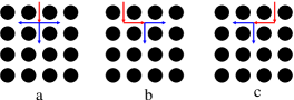
Figure 1: (Color on line). A model aggregate is composed of $l\times l$ identical particles on a square lattice. To break a bond between particles the energy $E_{\rm b}$ is needed. A crack propagates either away from the loaded surface (vertically-down on the plots), against the stress gradient, or laterally, but never along the gradient. All possible directions have equal probability. In the case (a) there exist three allowed directions, each with the probability $p_{3}=1/3$: one away from the surface and two lateral directions. In the cases (b) and (c) only two directions with the probability $p_{2}=1/2$ are possible, since crack can not move back or ”uphill” the load.

In Fig. 2 a typical fragmentation pattern, obtained with the use of the above fragmentation rules, is shown. Next, we analyze the statistical properties of debris.

 

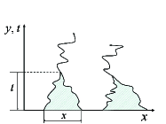
Figure 2: Left panel:  A typical fragmentation pattern. The aggregate, composed of one million particles on the $1\,000\times 1\,000$ lattice, is broken in 3958 pieces. The total breakage energy is $E_{\rm coll}=82\,010E_{\rm b}$, the crossing-factor is $E_{\rm cross}=3\,000~{}E_{\rm b}$. Right panel: The fragmentation model may be mapped on the one-dimensional model of diffusing and annihilating particles. The areas under the particle’s trajectories correspond to the fragment areas of the primary fragmentation model.

Fragment mass distribution. We define a fragment as a collection of constituent particles connected by adhesive bonds where a single particle consitutes a mass unit. Hence, for a fragment of $m$ particles we assign the mass $m$. We have performed numerical experiments, controlling the size of the aggregate, the total energy spent in the process and the crossing factor. To improve the fragments’ statistics we perform many runs with the same set of parameters.

Fig. 3 shows the fragment mass-distribution. The most part of the distribution, except for very large fragments, may be accurately fitted by the power-law

$$F(m)\propto m^{-\alpha}\,.$$ (1)

Interestingly, the exponent $\alpha\simeq 1.5$ is the same as in 2D egg-shell crushing experiments (Herrmann et al., 2006).

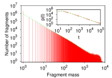
Figure 3: (Color online). Fragment mass distribution for a $100\times 100$ lattice matrix with total energy of $4\,000~{}E_{\rm b}$ and a crossing factor of $200~{}E_{\rm b}$. The data have been collected for $10\,000$ runs. The line represents a power law mass-distribution with an exponent $\simeq-3/2$. The inset shows the distribution function $P(x,t)\propto t^{-3/2}$, which gives the probability that two particles, initially separated by distance $x$, meet at time $t$; it illustrates the affinity of the two models (see the text). Points - numerical data for $x=20$, line - theory.

Analytical model. The observed power-law fragment size distribution may be obtained analytically, if we notice that the proposed fragmentation model may be mapped onto the one-dimensional model of diffusing and annihilating particles, where the particles correspond to the tips of the cracks. Indeed, the direction normal to the surface, that is, the direction of the most rapid decay of the stress, say axis $y$ (vertical downward in Fig. 1), may be mapped onto the time axis, since the reverse motion along this axis is forbidden. Then the location of the crack tips along the lateral direction, say along axis $x$ (horizontal in Fig. 1) corresponds to the location of fictitious ”particles” on the line. One step along $y$ axis corresponds to one time step, while one step along $x$ axis corresponds to a ”particle” jump on the line (without loss of generality we can assume unit time and space steps).

It is easy to see that the fragmentation model with the rules illustrated in Fig. 1 is equivalent to the following model: (i) Each particle on a line at each time step can remain at the same site with the probability $p_{0}=1/3$, move one site left or right with the probability $p_{1}=1/6$, two sites left or right with $p_{2}=1/12$, etc., $k$ sites left or right with the probability $p_{k}=1/(3\cdot 2^{k})$; note that $p_{0}+2\sum_{k}p_{k}=1$. (ii) When two particles meet, one of them annihilates while the other one continues to move with the same rules. (iii) The fragment sizes of the primary fragmentation model is equal to the area confined by the trajectories of the particles and the axis $x$, Fig. 2.

First we show that the ”particles” perform one-dimensional diffusion motion. Indeed, due to the lack of memory, each time step does not depend on the previous one (note that the original problem does have a memory with respect to previous steps). Therefore, the mean square displacement $<\left[\Delta x(t)\right]^{2}>$ is a sum of these quantities for each step, $\left<\Delta^{2}\right>$, where

$$\left<\Delta^{2}\right>=\sum_{l=0}^{\infty}2\,p_{l}l^{2}\,=\,\sum_{l=0}^{\infty}\frac{2\,l^{2}}{3\cdot 2^{l}}=4\,,$$

that is, $\left<\left[\Delta x(t)\right]^{2}\right>=4t=2Dt$. Hence, we have a diffusive motion with the diffusion coefficient $D=2$.

Now we compute the distribution of the fragments’ areas. These correspond to the areas of the figures on the $x-t$ plane confined by the $x$-axis and the diffusive trajectories of pairs of particles, which start to move at $t=0$, and meet at $t>0$; the initial separation of the particles is $x$. The area of the figures, that is, the fragment mass scales as $m\propto tx$. Hence, the mass distribution reads:

$$F(m)\simeq\int dx\int dt\delta(m-\gamma tx)\varkappa e^{-\varkappa\,x}P(x,t)\,,$$ (2)

where the coefficient $\gamma$ accounts for the surface density and a geometric factor (1/2 for triangles), which relates a fragment area and its dimensions $x$ and $t$. The coefficient $\varkappa$ is the line density of particles on the $x$ axis at the starting time $t=0$ (i.e. the density of crack tips which start at $y=0$); the random initial distribution of particles (crack tips) implies the Poisson distribution for the initial inter-particle distance, $\varkappa\exp(-\varkappa x)$.   $P(x,t)$ gives the probability of two diffusing particles, initially separated by distance $x$, to meet at time $t$; where one of the particles annihilates. $P(x,t)$ may be written as $P(x,t)=\frac{d}{dt}P_{\rm surv}(x,t)$, where

$$P_{\rm surv}(x,t)\!=\!\int_{0}^{\infty}\!\!\!\!\!\frac{1}{\sqrt{8\pi Dt}}\left(e^{-(y-x)^{2}/8Dt}-e^{-(y+x)^{2}/8Dt}\right)dy$$ (3)

is the survival probability, i.e. that both particles have not annihilated before time $t$, provided they started to diffuse at $t=0$ separated by the distance $x$. It is obtained from the solution of the diffusion problem with the adsorbing boundary condition for the relative motion of two particles, with the double diffusion coefficient $2D$ (see e.g. Krapivsky et al. (2010)). Indeed the integrand in Eq. (3) gives the probability distribution of the inter-particle distance $y$ at time $t$, if the initial separation was $x$, provided this probability is identically zero for $y=0$ (the annihilation condition). Integrating this probability over all distances $y>0$ gives the survival probability; differentiation of $P_{\rm surv}(x,t)$ with respect to time yields the probability that the particles meet exactly at time $t$. Substituting $P(x,t)=x\,\exp(-x^{2}/8Dt)/\sqrt{32Dt^{3}}$, obtained from Eq. (3) into Eq. (2), we arrive at the expansion,

$$F(m)=A_{0}m^{-3/2}+A_{1}m^{-5/2}+\ldots\,,$$ (4)

where $A_{0}=\gamma^{1/2}\Gamma(5/2)/8\varkappa^{3/2}$ and generally, $A_{l}=(-1)^{l}\Gamma(3l+5/2)(\gamma/\varkappa)^{3l+1/2}/(8\varkappa)(4\gamma)^{2l}l!$ is the coefficient at $m^{-(3/2+l)}$. Hence, Eq. (4) explains the power-law distribution (1) obtained numerically. The above expansion holds, however, not for very small masses, to keep the continuum diffusion approach valid, and not for very large masses, to ignore the effects of energy depletion and finite size effects of the fragmenting pattern.

Comparison with experiments. So far we considered the size distribution of fragments which mass is much smaller than the initial mass of the parent body. In this limit the numerically detected and explained power-law distribution coincides with the experimental one Herrmann et al. (2006).

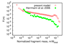
Figure 4: (Color online). Results of our model (red circles) compared with the experimental data (green squares) of Herrmann et al. (2006). In simulations we used a $600\times 600$ matrix, the total energy of $E_{\rm coll}=40\,000~{}E_{\rm b}$, the crossing-factor of $E_{\rm cross}=3\,000~{}E_{\rm b}$ and the number of runs is 200. Note the lack of any fitting or scaling of our data.

Surprisingly, our model can qualitatively and sometimes even semi-quantitatively reproduce the whole size distribution of fragments in the impact experiments. This is illustrated in Fig. 4 for the experiments of exploding egg-shells Herrmann et al. (2006) and in Fig. 5 for the colliding basalt spheres Nakamura and Fujiwara (1991). For the former case our model demonstrates an overall qualitatively correct behavior for $F(m)$, while for the latter case one can achieve a quantitative agreement with the most part of the experimental fragment size distribution. It is worth noting that the agreement is obtained without any fitting or scaling of our data. Moreover, the fact that our simple two-dimensional model can describe the fragmentation statistics for three-dimensional bodies indicates, that the main ingredients of our model - the diffusive propagation of cracks against the stress gradient and the depletion of energy with the cracks’ growth - are indeed the basic features of a fragmentation process.

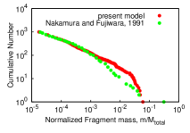
Figure 5: (Color online). Results of our model (red circles) compared with the experimental data (green circles) of Nakamura and Fujiwara (1991). In simulations we used a $80\times 80$ matrix, the total energy of $E_{\rm coll}=1500~{}E_{\rm b}$, the crossing-factor of $E_{\rm cross}=100~{}E_{\rm b}$; the number of runs is 10.

In conclusion we suggest a simple fragmentation model, based on a lattice random walk of a crack with propagation rules which mimic a real fragmentation process: A crack moves against (or laterally to) the stress gradient and the energy of the crack exhausts along its growth. We performed numerical simulations of the model and observed that the mass distribution of small and intermediate fragments obeys a power-law. The exponent of the power law, equal to $-3/2$, agrees with the reported experimental value. We develop an analytical theory which explains the nature of the power-law in the fragmentation statistics and demonstrate that the proposed model gives a qualitative description for the overall fragment size distribution observed in experiments.

References

- Grady and Lipkin (1980) D. E. Grady and J. Lipkin, Geophys. Res. Lett. 7, 255 (1980).
- Turcotte (1997) D. L. Turcotte, Fractals and Chaos in Geology and Geophysics (Cambridge, 1997).
- Michel et al. (2003) P. Michel, W. Benz, and D. C. Richardson, Nature (London) 421, 608 (2003).
- Nakamura et al. (2008) A. M. Nakamura, T. Michikami, N. Hirata, A. Fujiwara, R. Nakamura, M. Ishiguro, H. Miyamoto, H. Demura, K. Hiraoka, T. Honda, et al., Earth, Planets, and Space 60, 7 (2008).
- Thornton et al. (1996) C. Thornton, K. K. Yin, and M. J. Adams, J. Phys. D: Appl. Phys. 29, 424 (1996).
- Lankford and Blanchard (1991) J. Lankford and C. R. Blanchard, J. Mat. Sci. 26, 3067 (1991).
- Mott and Linfoot (1943) N. F. Mott and E. H. Linfoot, Tech. Rep., Ministry of Supply (1943).
- Grady (2006) D. E. Grady, Fragmentation of rings and shells: The legacy of N. F. Mott (Springer, 2006).
- Herrmann and Roux (1990) H. J. Herrmann and S. Roux, Statistical Models for the Fracture of Disordered Media (Elsevier, 1990).
- Nakamura and Fujiwara (1991) A. Nakamura and A. Fujiwara, Icarus 92, 132 (1991).
- Giblin et al. (1998) I. Giblin, G. Martelli, P. Farinella, P. Paolicchi, M. di Martino, and P. N. Smith, Icarus 134, 77 (1998).
- Arakawa (1999) M. Arakawa, Icarus 142, 34 45 (1999).
- Ryan (2000) E. V. Ryan, Annu. Rev. Earth Planet. Sci. 28, 367 (2000).
- Herrmann et al. (2006) H. J. Herrmann, F. K. Wittel, and F. Kun, Physica A 371, 59 (2006).
- Kun et al. (2006) F. Kun, F. K. Wittel, H. J. Herrmann, B. H. Kröplin, and K. J. Maloy, Phys. Rev. Lett. 96, 025504 (2006).
- Guettler et al. (2010) C. Guettler, J. Blum, A. Zsom, C. W. Ormel, and C. P. Dullemond, Astronomy and Astrophysics A56, 513 (2010).
- Timar et al. (2010) G. Timar, J. Blomer, F. Kun, and H. J. Herrmann, Phys. Rev. Lett. 104, 095502 (2010).
- Astrom et al. (2004) J. A. Astrom, F. Ouchterlony, and J. Linna, R. P. andTimonen, Phys. Rev. Lett. 92, 245506 (2004).
- Grady (2009) D. Grady, Int. J. Fract. pp. 1–15 (2009).
- Chang et al. (2002a) C. S. Chang, T. K. Wang, L. J. Sluys, and J. G. M. van Mier, Enginneering Fracture Mechanics 69, 1959 (2002a).
- Benz and Asphaug (1994) W. Benz and E. Asphaug, Icarus 107, 98 (1994).
- Bouchaud et al. (1993) J. P. Bouchaud, E. Bouchaud, G. Lapasset, and J. Planès, Phys. Rev. Lett. 71, 2240 (1993).
- Galybin and Dyskin (2004) A. N. Galybin and A. V. Dyskin, Int. J. Fracture 128, 95 (2004).
- Paolicchi et al. (1996) P. Paolicchi, A. Verlicchi, and A. Cellino, Icarus 121, 126 (1996).
- Chang et al. (2002b) C. S. Chang, T. K. Wang, L. J. Sluys, and J. G. M. van Mier, Enginneering Fracture Mechanics 69, 1941 (2002b).
- Kun and Herrmann (1999) F. Kun and H. J. Herrmann, Phys. Rev. E 59, 2623 (1999).
- Longaretti (1989) P.-Y. Longaretti, Icarus 81, 51 (1989).
- Spahn et al. (2004) F. Spahn, N. Albers, M. Sremcevic, and C. Thornton, Europhys. Lett. 67, 545 (2004).
- Sremčević et al. (2007) M. Sremčević, J. Schmidt, H. Salo, M. Seiß , F. Spahn, and N. Albers, Nature 449, 1019 (2007).
- Brilliantov et al. (2007) N. Brilliantov, N. Albers, F. Spahn, and T. Poeschel, Phys. Rev. E 76, 051302 (2007).
- Krapivsky et al. (2010) P. L. Krapivsky, S. Redner, and E. Ben-Naim, A Kinetic View of Statistical Physics (Cambridge University Press, 2010).