Prime knots whose arc index is smaller
than the crossing number

Abstract.

It is known that the arc index of alternating knots is the minimal crossing number plus two and the arc index of prime nonalternating knots is less than or equal to the minimal crossing number. We study some cases when the arc index is strictly less than the minimal crossing number. We also give minimal grid diagrams of some prime nonalternating knots with 13 crossings and 14 crossings whose arc index is the minimal crossing number minus one.

1. Arc presentation

A link can be embedded in a book of finitely many half planes in $\mathbb{R}^{3}$ so that each half plane intersects the link in a single arc. Such an embedding is called an arc presentation of the link. The minimal number of half planes among all arc presentations of a link is called the arc index of the link. The arc index of a link $L$ is denoted by $\alpha(L)$.

Suppose we have an arc presentation of a link $L$. In each half plane containing a single arc of $L$, we deform the arc into the union of two horizontal arcs and one vertical arc with the two end points fixed. Then we have a new arc presentation of $K$ which looks like the figure in the left of Figure 1. Relaxing the pairs of consecutive horizontal arcs off the axis, we obtain a diagram of $L$ as shown in the right of Figure 1. The new diagram is called a grid diagram. A grid diagram is a link diagram which is the union of a finitely many vertical strings and the same number of horizontal strings with the property that at every crossing the vertical string crosses over the horizontal string. The minimal number of vertical strings among all grid diagram of a link is equal to the arc index of the link.

Figure 1. An arc presentation of a trefoil knot and its grid diagram

For a link $L$, let $c(L)$, $F_{L}(v,z)$, and $\operatorname{spr}_{v}(F_{L}(v,z))$ denote the minimal crossing number, the Kauffman polynomial, and the $v$-spread of $F_{L}(v,z)$, i.e., the difference between the highest degree and the lowest degree of the variable $v$ in $F_{L}(v,z)$, respectively. Here we list some of the important known results about the arc index.

Proposition 1.1 (Cromwell).

Every link admits an arc presentation.

Theorem 1.2 (Cromwell).

If $L_{1}$ and $L_{2}$ are nontrivial links, then

$$\alpha(L_{1}\sharp L_{2})=\alpha(L_{1})+\alpha(L_{2})-2$$

Theorem 1.3 (Bae-Park).

If $L$ is a nonsplit link, then

$$\alpha(L)\leq c(L)+2$$

Theorem 1.4 (Morton-Beltrami).

For every link $L$, we have

$$\alpha(L)\geq\operatorname{spr}_{v}(F_{L}(v,z))+2$$

In particular, if $L$ is an alternating link, then

$$\alpha(L)\geq c(L)+2$$

Theorem 1.5 (Jin-Park).

A prime link $L$ is nonalternating if and only if

$$\alpha(L)\leq c(L)$$

Theorem 1.2 allows us to focus on prime links. Theorem 1.3 and Theorem 1.4 together imply that the arc index equals the minimal crossing number plus two for nonsplit alternating links.

Theorem 1.4 and Theorem 1.5 together imply Corollary 1.6 which leads us to conclude that, for prime nonalternating links, if the $v$-spread of the Kauffman polynomial plus two is equal to the minimal crossing number, then it is equal to the arc index.

Corollary 1.6.

A prime nonalternating link $L$ satisfies the inequality

$$\operatorname{spr}_{v}(F_{L}(v,z))+2\leq\alpha(L)\leq c(L)$$

Table 1 shows the number of prime nonalternatings knots up to 16 crossings and those satisfying both equalities in Corollary 1.6.

minimal crossing	prime nonalternating	prime nonalternating knots with
number $n$	knots with $n$ crossings	$n$ crossings and $v\text{-spread}+2=n$
08	0,000,003	000,002
09	0,000,008	000,006
10	0,000,042	000,032
11	0,000,185	000,135
12	0,000,888	000,627
13	0,005,110	003,250
14	0,027,436	015,735
15	0,168,030	083,106
16	1,008,906	423,263

Table 1. Nonalternating primes knots whose arc index is determined by Corollary 1.6

In this article, we give three conditions for diagrams of a knot or link to have the arc index smaller than the number of crossings. For each of these conditions we give a list of 13 crossing knots satisfying the condition and having the arc index 12.

2. The Knot-spoke diagram approach due to Bae and Park

Now we briefly describe the methods used in the proofs of Theorems 1.3 and 1.5.

A wheel diagram is a finite plane graph of straight edges which are incident to a single vertex [1]. The projection of an arc presentation of a knot or a link into the $xy$-plane is of this shape. For a wheel diagram with $n$ edges to represent a knot or a link, each edge is labeled with an unordered pair of distinct integers, $1,2,\ldots,n$, so that each of the integers appears exactly twice. These numbers indicate the relative $z$-levels of the end points of the corresponding arcs. Since there are only finitely many choices for labelings, there are only finitely many knots and links for each arc index.

Figure 2. Wheel Diagrams

A knot-spoke diagram $D$ is a finite connected plane graph satisfying the two conditions:

1. There are three kinds of vertices in $D$; a distinguished vertex $v_{0}$ with valency at least four, 4-valent vertices, and 1-valent vertices.

2. Every edge incident to a 1-valent vertex is also incident to $v_{0}$. Such an edge is called a spoke.

A wheel diagram is a knot-spoke diagram without any non-spoke edges. A knot-spoke diagram $D$ is said to be prime if no simple closed curve meeting $D$ in two interior points of edges separates multi-valent vertices into two parts. A multi-valent vertex $v$ of a knot-spoke diagram $D$ is said to be a cut-point if there is a simple closed curve $S$ meeting $D$ in the single point $v$ and separating non-spoke edges into two parts.

Figure 3. Knot-spoke diagrams

Figure 4. Prime diagram and non-prime diagram

Figure 5. A cut-point

Notice that a cut-point free knot-spoke diagram with more than one non-spoke edges cannot have a loop, and that if a prime knot-spoke diagram $D$ has a cut-point, then the distinguished vertex $v_{0}$ must be the cut-point with valency bigger than four.

To obtain types of a knot or a link which can be projected onto a knot-spoke diagram $D$, we need to assign relative heights of the endpoints of edges of $D$ in the following way.

1. At every 4-valent vertex, pairs of opposite edges meet in two distinct levels so that a knot-crossing is created.

2. If the distinguished vertex $v_{0}$ is incident to $2a$ non-spoke edges and $b$ spokes, then its small neighborhood is the projection of $n=a+b$ arcs at distinct levels whose relative $z$-levels can be specified by the numbers $1,\cdots,n$. Every spoke is understood as the projection of an arc on a vertical plane whose endpoints project to $v_{0}$.

Local diagram of $D$ near $e$     Local diagram of $D_{e}$ near $v_{0}$

Figure 6. Contraction of an edge in $D$

Let $e$ be an edge of a cut-point free knot-spoke diagram $D$ as in Figure 6. The knot-spoke diagram $D_{e}$ is obtained by contracting $e$ and then replacing each simple loop created from $\bar{e}$ or $\bar{e}^{\prime}$ by a spoke. The relative $z$-levels of the edges $e^{\prime},\bar{e},\bar{e}^{\prime}$ at $v_{0}$ in $D_{e}$ are easily decided by the $z$-level of $e$ at $v_{0}$ and the type of the crossing $v_{1}$ so that we do not need to keep track of the $z$-levels in detail for the proof of Theorem 1.3. But for the proof of Theorem 1.5 we need to pay attention to some spokes corresponding to nonalternating edges.

Lemma 2.1 (Bae-Park).

Let $D$ be a prime knot-spoke diagram without cut-points. Suppose that $D$ has at least two multi-valent vertices. Then there are at least two non-loop non-spoke edges e and f, incident to $v_{0}$, such that the knot-spoke diagrams $D_{e}$ and $D_{f}$ have no cut-points.

A loop in a knot-spoke diagram is said to be simple if the other non-spoke edges are in one side of it. By the above lemma, the edge contractions can be performed repeatedly, without creating a cut-point, until we obtain a knot-spoke diagram with $c(D)$ spokes and only one non-spopke edge which is a non-simple loop where $c(D)$ is the number of crossings in $D$. Notice that the following three properties are preserved.

1. $D$ and $D_{e}$ represent the same knot or link.

2. The sum of the number of regions divided by the non-spoke edges and the number of spokes is unchanged.

3. $D_{e}$ is prime if $D$ is prime.

The last non-spoke edge, which is a loop, is being folded to create two extra spokes to show the inequality $\alpha(L)\leq c(L)+2$ of Theorem 1.3.

$\Longrightarrow$ 

Figure 7. Folding the last non-spoke edge

In the case of nonalternating diagrams, there are at least two removable spokes so that the inequality of Theorem 1.5 can be proved. The edges to be contracted must be chosen carefully to make nonalternating edges into removable spokes. Therefore a more elaborate method than Lemma 2.1 is needed to avoid cut-point. The following lemma plays an important role for this purpose.

Lemma 2.2 (Jin-Park).

Let $D$ be a prime cut-point free knot-spoke diagram and let $e$ be an edge incident to $v_{0}$ and to another $4$-valent vertex $v_{1}$ such that $D_{e}$ has a cut-point. Then there exists a simple closed curve $S_{e}$ satisfying the following conditions.

1. $D_{e}\cap S_{e}=v_{0}$

2. $S_{e}$ separates $\bar{e}$ and $\bar{e}^{\prime}$ where the four edges incident to $v_{1}$ in $D$ are labeled with $e,\bar{e},e^{\prime},\bar{e}^{\prime}$ as in Figure 6.

3. $S_{e}$ separates $D_{e}$ into two knot-spoke diagrams $\bar{D}$ and $\bar{D}^{\prime}$ containing $\bar{e}$ and $\bar{e}^{\prime}$, respectively. Futhermore $\bar{D}^{\prime}$ is prime and cut-point free, and there is a sequence of non-spoke edges $e_{1},e_{2},\cdots,e_{k}$ of $D$ not contained in $\bar{D}^{\prime}$ such that the knot-spoke diagram $D_{{e_{1}}{e_{2}}{\cdots}{e_{k}}}$ is identical with $\bar{D}^{\prime}$ on non-spoke edges in one side of $S_{e}$ and has only spokes in the other side.

3. Filtered Spanning Trees

Figure 8. A filtered spanning tree and its successive closures

Figure 9. Contraction of a triangular region using a doubly-good edge

Instead of collapsing edges of a diagram $D$ in sequence to obtain a wheel diagram, we consider the tree in $D$ consisting of the edges to be contracted. With this new approach, we describe the method used in the proof of Theorem 1.5.

Let $D$ be a knot diagram. We may consider $D$ as a connected $4$-valent plane graph with $c(D)$ vertices and $2\,c(D)$ edges. A filtered tree of $D$ is an increasing sequence $T_{0}\subset T_{1}\subset T_{2}\subset\cdots\subset T_{k}$ of subgraphs of $D$ such that each $T_{i}$ is a tree containing $i$ edges. The edges of $T_{k}$ are ordered by the filtering. On the other hand, if the edges of a tree $T$ are ordered so that each of their successive unions is connected, the ordering gives rise to a filtered tree structure on $T$. If a tree $T$ is prescribed with such an ordering we can consider $T$ as a filtered tree.

The closure of $T_{i}$, denoted by $\overline{T}_{i}$, is the subgraph of $D$ obtained from $T_{i}$ by adding the edges which are incident to $T_{i}$ at both ends. An edge $f$ of $\overline{T}_{i}\setminus T_{i}\subset D$ is said to be good if it meets the edge $e_{i}=T_{i}\setminus T_{i-1}$ transversely at the vertex not contained in $T_{i-1}$. An edge $f$ of $\overline{T}_{i}\setminus T_{i}\subset D$ is said to be bad if it is an extension of the edge $e_{i}$ at the vertex not contained in $T_{i-1}$. In Figure 8, good edges and bad edges are labeled with the letters $g$ and $b$, respectively.

Let $T_{0}\subset T_{1}\subset\cdots\subset T_{i}=T$ be a filtered tree in a diagram $D$ which does not span $D$. A simple arc $\Gamma$, which does not form a bigon together with a single edge of $D$, is called a cutting arc of $T$ if $\Gamma\cap D$ consists of two distinct vertices $p\in T_{i}\setminus T_{i-1}$ and $c\in T_{i-1}$ such that the simple closed curve in $\Gamma\cup T_{i}$ separates edges of $D\setminus\overline{T}_{i}$ into two parts. We say that the filtered tree $T$ is good if, for each $j\leq i$, the subtree $T_{0}\subset T_{1}\subset\cdots\subset T_{j}$ of $T$ has no cutting arc and $\overline{T}_{j}$ has no bad edge.

If a filtered tree of $D$ terminates with a spanning tree of $D$, we call it a filtered spanning tree of $D$. As every spanning tree of $D$ has $c(D)-1$ edges, a filtered spanning tree of $D$ is of the form $T_{0}\subset T_{1}\subset T_{2}\subset\cdots\subset T_{c(D)-1}$. A filtered spanning tree $T_{0}\subset T_{1}\subset T_{2}\subset\cdots\subset T_{c(D)-1}$ is said to be good if each $T_{i}$ is good for $i<c(D)-1$ and if $T_{c(D)-1}$ has no cutting arc. Notice that $\overline{T}_{c(D)-1}$ has a bad edge.

We rephraise the statement of Theorem 1.3 in the following way.

Theorem 3.1 (Theorem 1.3 rephrased).

A prime link diagram $D$ admits a good filtered spanning tree and therefore one can obtain an arc presentation with $c(D)+2$ arcs.

Figure 10. Good edges and a bad edge

A good edge $e\subset\overline{T}_{i}\setminus\overline{T}_{i-1}$ is said to be doubly good if it is a nonalternating edge and the simple closed curve in $T_{i}\cup e$ has only good edges of $T_{j}$, $j\leq i$, in one side. A doubly good edge $e\subset\overline{T}_{i}\setminus\overline{T}_{i-1}$ and the two edges $e_{i}=T_{i}\setminus T_{i-1}$, and $e_{i-1}=T_{i-1}\setminus T_{i-2}$ together bound a nonalternating triangular region in $D/T_{i-2}$, as shown in Figure 9, which can be contracted to reduce the number of regions by one without increasing the number of spokes. Thus the existence of one doubly good edge leads to an arc presentation with one less arcs than the process described in the property (6) of page 6.

Theorem 3.2 (Theorem 1.5 rephrased).

A prime nonalternating diagram $D$ of a link has a good filtered spanning tree which has at least two doubly good edges so that $D$ has an arc presentation with $c(D)$ arcs.

In Figure 10, the sequence $e_{1},e_{2},\ldots,e_{11}$ gives rise to a filtered spanning tree $T_{i}=v_{0}\cup e_{1}\cup\cdots\cup e_{i}$, $i=0,\ldots,11$. The edges $A$ through $L$ are good and the edge $M$ is bad. The three edges $A$, $F$ and $I$ are doubly good if they are nonalternating.

The following proposition is immediate from the definition of good filtered trees.

Proposition 3.3.

Let $T_{0}\subset T_{1}\subset\cdots\subset T_{m}$ be a non-spanning good filtered tree in a prime diagram $D$. Let $e$ be an edge in $D$ such that $T_{m}\cap e$ is a single vertex, so that $T_{m}\cup e$ is a tree. If $T_{0}\subset T_{1}\subset\cdots\subset T_{m}\subset(T_{m}\cup e)$ is not a good filtered tree, then $\overline{T_{m}\cup e}$ has a bad edge or a sufficiently small neighborhood of $\overline{T_{m}\cup e}$ has disconnected exterior in $D$.

Figure 11. Extending $T_{m}$ along $e$ in $D$

Suppose that $T_{0}\subset T_{1}\subset\cdots\subset T_{m}$ and $e$ are as in the hypothesis of Proposition 3.3 and that $T_{0}\subset T_{1}\subset\cdots\subset T_{m}\subset(T_{m}\cup e)$ is not a good filtered tree. In Figure 11, $v$ is the vertex of $e$ belonging to $T_{m}$ and $p$ is the other vertex of $e$. The three edges $e^{\prime}$, $\bar{e}$, $\bar{e}^{\prime}$ are incident to $e$ at $p$ and $R$ is a region of $D$ whose boundary contains $e$ and $\bar{e}^{\prime}$. Proposition 3.3 implies that there are three cases to consider:

1. $e^{\prime}$ is a bad edge of $\overline{T_{m}\cup e}$ joining $p$ and a vertex $c$ of $T_{m}$.

2. There is a simple arc $\Gamma_{p}$ contained in a single region of $D$ joining $p$ and a vertex $c$ of $T_{m}$ such that the unique cycle $\overline{\Gamma}_{p}$ in $T_{m}\cup e\cup\Gamma_{p}$ does not enclose the region $R$ but encloses the edges $e^{\prime}$ and $\bar{e}$.

3. There is a simple arc $\Gamma_{p}$ as in (B2) except that $\overline{\Gamma}_{p}$ does not enclose $e^{\prime}$.

Figure 12. Three bad cases for $T_{m}\cup e$

For each of the above cases, we say that $T_{m}\cup e$ is a (B$n$)-extension of $T_{m}$, $n=1,2,3$. If $T_{0}\subset T_{1}\subset\cdots\subset T_{m}\subset(T_{m}\cup e)$ is a good filtered (spanning) tree, we say that $T_{m}\cup e$ is a good extension of $T_{m}$.

4. Main Theorems

Before we state our main theorems, we give several lemmas and corollaries. The first two lemmas are translations of the two lemmas written in the language of knot-spoke diagrams into the ones written in the language of filtered trees.

Lemma 4.1 (Lemma 2.1 rephrased).

Let $D$ be a prime knot diagram with $c(D)$ crossings and let $T_{0}\subset T_{1}\subset\cdots\subset T_{m}$ be a non-spanning good filtered tree in $D$. Then there are two edges $e$ and $f$ in $D\setminus\overline{T}_{m}$ such that $T_{m}\cup e$ and $T_{m}\cup f$ are good extensions of $T_{m}$.

Lemma 4.2 (Lemma 2.2 rephrased).

Let $T_{0}\subset T_{1}\subset\cdots\subset T_{m}$ be a good filtered tree in a prime diagram $D$ with $m<c(D)-2$. Let $e$ be an edge in $D$ such that $T_{m}\cap e$ is a single vertex, say $v$. Suppose that $T_{m}\cup e$ is not a good extension of $T_{m}$. Then there exists a simple closed curve $S$ satisfying the following conditions.

1. $D\cap S$ is a simple arc which is the union of $e$ and some edges of $T_{m}$.

2. $S$ separates $\bar{e}$ and $\bar{e}^{\prime}$ where the four edges incident to $p$, the endpoint of $e$ other than $v$, are labeled with $e,\bar{e},e^{\prime},\bar{e}^{\prime}$ as in Figure 11.

3. $S$ separates $D$ into two subgraphs $\bar{D}$ and $\bar{D}^{\prime}$ containing $\bar{e}$ and $\bar{e}^{\prime}$, respectively and satisfying $\bar{D}\cap\bar{D}^{\prime}=D\cap S$. Futhermore there is a sequence $e_{1},e_{2},\cdots,e_{k}$ of $D\setminus\ (\bar{D}^{\prime}\cup\overline{T}_{m})$ such that $T_{0}\subset\cdots\subset{T_{m}}\subset{T_{m}\cup e_{1}}\subset\cdots\subset{T_{m}\cup e_{1}\cup\cdots\cup e_{k}}$ is a good filtered tree and $D\setminus{\overline{T_{m}\cup e_{1}\cdots\cup e_{k}}}=\bar{D}^{\prime}\setminus\overline{T_{m}\cup e}$.

Remark. If $T_{m}\cup e$ is a (B3)-extension of $T_{m}$, the sequence $e_{1},e_{2},\cdots,e_{k}$ of Lemma 4.2 can be chosen so that $e_{k}=e$. See the original proof of Lemma 2.2 [6, Proposition 8].

The closure of a region divided by a diagram $D$ is called a face of $D$. Let $T_{0}\subset T_{1}\subset T_{2}\subset\cdots\subset T_{j}$ be a non-spanning filtered tree of $D$. If $T_{j}$ has a cutting arc $\Gamma_{p}$, we may assume that it is innermost, in the following sense: Let $F$ be the face of $D$ containing $\Gamma_{p}$ and let $\Delta\subset F$ be the disk enclosed by the unique cycle of $T_{j}\cup\Gamma_{p}$ satisfying $\partial\Delta\subset\partial F\cup\Gamma_{p}$. Then any cutting arc of $T_{j}$ contained in $\Delta$ is isotopic to $\Gamma_{p}$.

The following lemma asserts that two innermost cutting arcs are essentially disjoint. We omit the proof.

Lemma 4.3.

Let $T_{0}\subset T_{1}\subset\cdots\subset T_{j}$ be a non-spanning filtered tree of $D$. If $\Gamma_{p}$ and $\Gamma_{q}$ are innermost cutting arcs of $T_{i}$ and $T_{j}$, respectively, for some $i<j$, then we can isotope $\Gamma_{p}$ and $\Gamma_{q}$ so that they do not intersect in their interiors.

If $p$ and $q$ are the two vertices of an edge $e$ of $D$, we write $e=\overline{pq}$, even in the case that there is another edge joining $p$ and $q$ if we understand which is $e$.

Lemma 4.4.

Let $T_{0}\subset T_{1}\subset\cdots\subset T_{m}$ be a non-spanning good filtered tree of $D$ and let $\overline{sp}$, $\overline{pq}$, and $\overline{qr}$ be three consecutive edges along the boundary $\partial F$ of a face $F$ of $D$. Suppose that $\partial F\cap T_{m}\neq\emptyset$ and $\overline{pq}\cap T_{m}=\emptyset$. Then we can always construct a sequence of successive good extensions $T_{m+1}\subset\cdots\subset T_{m+k}$ of $T_{m}$ such that the closure $\overline{T}_{m+k}$ contains all edges of $\partial F$ except $\overline{sp}$, $\overline{pq}$, and $\overline{qr}$.

Proof.

We construct a sequence of successively extended filtered tree $T_{m+1}\subset\cdots\subset T_{m+k}$ of $T_{m}$ along the edges of $\partial F$ so that $T_{m+k}$ contains all vertices of $\partial F$ except $p$ and $q$. If $T_{m+i}$ is not a good extension for some $i$, we apply Lemma 4.2 to obtain a larger good filtered tree $T^{\prime}$ not containing the edges $\overline{sp}$, $\overline{pq}$, and $\overline{qr}$, and continue. ∎

The following lemma is an immediate consequence of related definitions.

Lemma 4.5.

Let $T_{0}\subset T_{1}\subset\cdots\subset T_{m}$ be a non-spanning good filtered tree of $D$ and let $\overline{sp}$, $\overline{pq}$, and $\overline{qr}$ be three consecutive edges along the boundary $\partial F$ of a face $F$ of $D$. Suppose that $\overline{pq}$ is a nonalternating edge and $\partial F\setminus\{\overline{sp},\overline{pq},\overline{qr}\}\subset\overline{T}_{m}$. Then $\overline{pq}$ becomes a doubly good edge of $\overline{T}_{m+2}$ if the following two conditions are satisfied:

1. $T_{m+1}=T_{m}\cup{\overline{sp}}$ is a good extension of $T_{m}$.

2. $T_{m+2}=T_{m+1}\cup\overline{rq}$ is a good extension of $T_{m+1}$.

Corollary 4.6.

Let $T_{m}$, $F$, $\overline{sp}$, $\overline{pq}$, and $\overline{qr}$ be as in Lemma 4.5. Suppose that the two conditions below are satisfied:

1. $T_{m+1}=T_{m}\cup{\overline{sp}}$ is a (B3)-extension of $T_{m}$ so that there is a tree $T^{\prime}$ which has a good extension $T^{\prime}\cup\overline{sp}$ containing $T_{m+1}$. (See the remark following Lemma 4.2.)

2. ${T^{\prime}}\cup{\overline{sp}}\cup{\overline{rq}}$ is a good extension of ${T^{\prime}}\cup{\overline{sp}}$.

Then $\overline{pq}$ is a doubly good edge of $\overline{T^{\prime}\cup\overline{sp}\cup\overline{rq}}$.

Lemma 4.7.

Let $F$ be a face of a minimal crossing diagram $D$ of a prime knot such that $\partial F$ contains a nonalternating edge $\overline{pq}$. We may label the vertices of $\partial F$ as $v_{0},v_{1},\ldots,v_{n-2}=q,v_{n-1}=p$, cyclically around $F$, for some $n\geq 3$. Then there is a good filtered tree $T_{0}\subset\cdots\subset T_{m}$ such that $T_{0}=v_{0}$, $v_{i}\in T_{m}$, $i=0,\ldots,n-3$ and $T_{m+1}$ is a good extension of $T_{m}$ along $\overline{v_{n-3}q}\subset\partial F$. Furthermore if the extension $T_{m+2}$ of $T_{m+1}$ along $\overline{v_{0}p}\subset\partial F$ is not (B3), then $\overline{pq}$ is a doubly good edge of $\overline{T}_{m+2}$.

Proof.

We extend $T_{0}$ repeatedly along the edges $\overline{v_{i-1}v_{i}}$, $i=1,\ldots,n-3$. These extensions are neither (B1) nor (B2) since $D$ is prime. If a (B3)-extension occurs, then, by Lemma 4.2, we can insert more edges before the extension to obtain a good extension along the same edge. Continuing in this manner, we obtain the good extension $T_{m+1}=T_{m}\cup\overline{v_{n-3}q}$ of $T_{m}$. Since $D$ is prime, the extension is neither (B1) nor (B2). This completes the proof. ∎

Corollary 4.8.

Suppose that the hypothesis of Lemma 4.7 holds and that $v_{0}$ and $p$ are two vertices of a bigonal face adjacent to $F$. Then $\overline{pq}$ is a doubly good edge of $\overline{T}_{m+2}$.

Proof.

In this case, the extension $T_{m+2}$ of $T_{m+1}$ mentioned in Lemma 4.7 cannot be (B3). ∎

Let $n\geq 2$. An $(n,1)$-tangle is an alternating tangle diagram of $n+1$ crossings whose projection is as shown in Figure 13 $(a)$. A nonalternating knot diagram $D$ is said to be $(n,1)$-nonalternating if it can be decomposed of two alternating tangles one of which is an $(n,1)$-tangle. Let $n\geq 1$. We can define an $n$-tangle and $n$-nonalternating diagram in a similar manner, using Figure 13 $(b)$. A $1$-tangle is a single crossing and a $1$-nonalternating diagram is also called an almost alternating diagram.

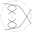
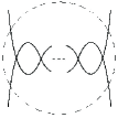
(a) $(n,1)$-tangle     (b) $n$-tangle       (c) $1$-tangle

Figure 13. Projections of various alternating tangles

Now we are ready to state our main theorems.

Theorem 4.9.

Let $n\geq 2$ and let $D$ be a prime $(n,1)$-nonalternating minimal crossing knot diagram having a nonalternating triangular face $F_{3}$. Suppose that faces $F_{1}$, $F_{2}$, $F_{3}$, $F$, edges $e_{1}$, $e_{2}$ and a vertex $q$ of $D$ are labeled as in Figure 14. Then $\alpha(D)<c(D)$ if $D$ satisfies the two conditions below:

1. The face $F$ satisfies ${e_{1}\cup e_{2}}\subset\partial F$ and $F\cap{(F_{1}\cup F_{2})}=\emptyset$.

2. There are two vertices $v\in{\partial F\cup\{q\}}$, $w\in{\partial F_{2}}$ and a string $a_{vw}$ of $D$ joining $v$ and $w$ such that no edge of $\partial F_{1}\cup\partial F_{3}$ is contained in $a_{vw}$.

Figure 14. $(2,1)$-nonalternating diagram

Theorem 4.10.

Let $n\geq 2$ and let $D$ be a prime, $n$-nonalternating and minimal crossing knot diagram having a nonalternating triangular face $F_{3}$. Suppose that faces $F_{1}$, $F_{2}$, $F_{3}$, $F$, edges $e_{1}$, $e_{2}$ and a vertex $q$ of $D$ are labeled as in Figure 15. Then $\alpha(D)<c(D)$ if $D$ satisfies the three conditions below:

1. The face $F$ satisfies ${e_{1}\cup e_{2}}\subset\partial F$ and $F\cap{(F_{1}\cup F_{2})}=\emptyset$.

2. There are two vertices $v\in\partial F$, $w\in{\partial F_{2}\setminus\{q\}}$ and a string $a_{vw}$ of $D$ joining $v$ and $w$ such that no edge of $\partial F_{1}\cup\partial F_{2}\cup\partial F_{3}$ is contained in $a_{vw}$.

3. $\partial{F_{2}}$ consists of at least $n+3$ edges.

Figure 15. $2$-nonalternating diagram

Theorem 4.11.

Let $D$ be a prime, almost alternating, and minimal crossing knot diagram having a nonalternating triangular face $F_{3}$. Suppose that faces $F_{1}$, $F_{2}$, $F_{3}$, an edge $e$ and a vertex $q$ of $D$ are labeled as in Figure 16. Let $F$ be the union of two faces containing $e$ in the intersection of their boundaries. Then $\alpha(D)<c(D)$ if $D$ satisfies the two conditions below:

1. $F\cap{(F_{1}\cup F_{2})}=\{q\}$

2. There are two vertices $v\in{\partial F}$, $w\in{\partial F_{2}}$ and a string $a_{vw}$ of $D$ joining $v$ and $w$ such that no edge of $\partial F_{1}\cup\partial F_{3}$ is contained in $a_{vw}$.

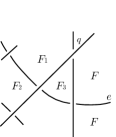
Figure 16. almost alternatingdiagram

5. Proofs of Main Theorems

5.1. Proof of Theorem 4.9

We give a proof of the case $n=2$. It can be easily adapted for $n>2$.

Let $D^{\prime}$ be the diagram obtained from $D$ by a type $3$ Reidemeister move over the face $F_{3}$. Some vertices, edges, and faces of $D^{\prime}$ are labeled as in Figure 17. The vertices $v_{1},\ldots,v_{7}$ are all distinct except in the case that $\partial F_{1}$ of $D$ consists of only four edges where $v_{1}=v_{2}$. The two conditions of the theorem are modified to the following conditions on the diagram $D^{\prime}$:

1. The face $F^{\prime}$ satisfies ${e_{1}^{\prime}\cup e_{2}^{\prime}}\subset\partial{F^{\prime}}$ and $F^{\prime}\cap{(F_{1}^{\prime}\cup F_{2}^{\prime})}=\emptyset$

2. There are two vertices $v\in{\partial F^{\prime}}$ and $w\in{\partial F_{2}^{\prime}}$ and a string $a_{vw}$ of $D$ joining $v$ and $w$ such that no edge of $\partial F_{1}^{\prime}\cup\partial F_{3}^{\prime}$ is contained in $a_{vw}$. The case $a_{vw}=\overline{v_{7}v_{5}}$ is excluded.

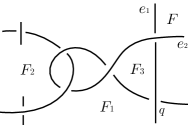
$\Longrightarrow$ 

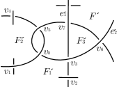
Figure 17. A type 3 Reidemeister move

In this proof, we will construct a filtered tree whose successive closures gradually contain $\partial F_{1}^{\prime},\partial F_{2}^{\prime}$ and $\partial F_{3}^{\prime}$ without introducing bad edges and cutting arcs. During the construction, the nonalternating edges $\overline{v_{2}v_{3}}$, $\overline{v_{4}v_{5}}$ and $\overline{v_{6}v_{7}}$ will appear as doubly good edges in this order.

Step 1. The edge $\overline{v_{2}v_{3}}$ becomes doubly good.

Let $v_{2}^{\prime}$ be the vertex of $\partial F^{\prime}_{1}$ such that $v_{0},v_{3},v_{2},v^{\prime}_{2}$ are adjacent along $\partial F^{\prime}_{1}$ in this order. Applying Lemma 4.7, we obtain a good filtered tree $v_{0}=T_{0}\subset\cdots\subset T_{m}$ such that $T_{m}$ contains all vertices of $\partial F^{\prime}_{1}$ except $v_{2}$ and $v_{3}$, and its good extension $T_{m+1}$ along $\overline{v^{\prime}_{2}v_{2}}$. Extending once more along $\overline{v_{0}v_{3}}$, we obtain $T_{m+2}$. The edge $\overline{v_{6}v_{7}}$ obstructs the existence of a (B3) cutting arc for $T_{m+2}$. By Lemma 4.7, $\overline{v_{2}v_{3}}$ is doubly good in $\overline{T}_{m+2}$.

Step 2. The edge $\overline{v_{4}v_{5}}$ becomes doubly good.

Let $v_{4}^{\prime}$ be the vertex of $\partial F^{\prime}_{2}$ such that $v_{0},v_{5},v_{4},v^{\prime}_{4}$ are adjacent along $\partial F^{\prime}_{2}$ in this order. By Lemma 4.4, we have a sequence of good extensions $T_{m+2}\subset\cdots\subset T_{n}$ such that $\overline{T}_{n}$ contains all edges of $\partial F^{\prime}_{2}$ except $\overline{v^{\prime}_{4}v_{4}}$, $\overline{v_{4}v_{5}}$ and $\overline{v_{5}v_{0}}$. By ($2^{\prime}$) and by $D$ being prime and minimal, the extension $T_{n}\cup\overline{v^{\prime}_{4}v_{4}}$ cannot be (B1) nor (B2). If it is (B3) then, applying Lemma 4.7, we can replace $T_{n}$ by a larger tree $T_{n^{\prime}}$ so that $T_{n^{\prime}}\cup\overline{v^{\prime}_{4}v_{4}}$ is a good extension. By the same reasons, the extension $T_{n^{\prime}+2}=T_{n^{\prime}}\cup\overline{v^{\prime}_{4}v_{4}}\cup\overline{v_{0}v_{5}}$ is not (B1) nor (B2). The edge $\overline{v_{3}v_{7}}$ obstructs the existence of a (B3) cutting arc for $T_{n^{\prime}+2}$. By Lemma 4.7, $\overline{v_{4}v_{5}}$ is doubly good in $\overline{T}_{n^{\prime}+2}$.

Step 3. The edge $\overline{v_{6}v_{7}}$ becomes doubly good.

By ($1^{\prime}$) and by $D$ being prime and minimal, the extension $T_{n^{\prime}+2}\cup\overline{v_{3}v_{6}}$ cannot be (B1) nor (B2). If it is (B3) then, applying Lemma 4.7, we can replace $T_{n^{\prime}+2}$ by a larger tree $T_{n^{\prime\prime}}$ so that $T_{n^{\prime\prime}}\cup\overline{v_{3}v_{6}}$ is a good extension. Now we consider the extension $T_{n^{\prime\prime}+2}=T_{n^{\prime\prime}}\cup\overline{v_{3}v_{6}}\cup\overline{v_{3}v_{7}}$. It cannot be (B1) by one of the conditions ($1^{\prime}$), ($2^{\prime}$), $D^{\prime}$ being prime and minimal, depending on the location of the endpoint $c\in T_{n^{\prime\prime}}\cup\overline{v_{3}v_{6}}$ of the bad edge $e_{1}^{\prime}$. It cannot be (B2) nor (B3) by one of the conditions ($1^{\prime}$), ($2^{\prime}$) and $D^{\prime}$ being prime, depending on the location of the endpoint $c\in T_{n^{\prime\prime}}\cup\overline{v_{3}v_{6}}$ of the cutting arc $\Gamma_{p}$ where $p=v_{7}$. By Lemma 4.5 and Corollary 4.6, the nonalternating edge $\overline{v_{6}v_{7}}$ a is doubly good edge of $\overline{T}_{n^{\prime\prime}+2}$.

5.2. Proof of Theorem 4.10

Let $D^{\prime}$ be the diagram obtained from $D$ by a type $3$ Reidemeister move over the face $F_{3}$. Some vertices and faces of $D^{\prime}$ are labeled as in Figure 18. The vertices $v_{0},\ldots,v_{6}$ are all distinct. The three conditions of the theorem are modified to the following conditions on the diagram $D^{\prime}$:

1. The face $F^{\prime}$ satisfies ${e_{1}^{\prime}\cup e_{2}^{\prime}}\subset\partial{F^{\prime}}$ and $F^{\prime}\cap{(F_{1}^{\prime}\cup F_{2}^{\prime})}=\emptyset$

2. There are two vertices $v\in{\partial F^{\prime}}$ and $w\in{\partial F_{2}^{\prime}}$ and a string $a_{vw}$ of $D$ joining $v$ and $w$ such that no edge of $\partial F_{1}^{\prime}\cup\partial F_{2}^{\prime}\cup\partial F_{3}^{\prime}$ is contained in $a_{vw}$. The case $a_{vw}=\overline{v_{6}v_{2}}$ is excluded.

3. $\partial F_{2}^{\prime}$ consists at least $n+2$ edges.

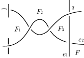
$\Longrightarrow$ 

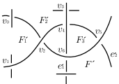
Figure 18. A type 3 Reidemeister move

Similarly as in the proof of Theorem 4.9, we construct a filtered tree whose successive closures gradually contain $\partial F_{1}^{\prime},\partial F_{2}^{\prime}$ and $\partial F_{3}^{\prime}$ without introducing bad edges and cutting arcs. During the construction, the nonalternating edges $\overline{v_{1}v_{2}}$, $\overline{v_{3}v_{4}}$ and $\overline{v_{5}v_{6}}$ will appear as doubly good edges. We skip the detail.

5.3. Proof of Theorem 4.11

Let $D^{\prime}$ be the diagram obtained from $D$ by a type $3$ Reidemeister move over the face $F_{3}$. Some vertices and faces of $D^{\prime}$ are labeled as in Figure 19. The vertices $v_{0},\ldots,v_{5}$ are all distinct. Let $F^{\prime}$ be the union of two faces containing $e^{\prime}$ in the intersection of their boundaries. The two conditions of the theorem are modified to the following conditions on the diagram $D^{\prime}$:

1. $F^{\prime}\cap{(F_{1}^{\prime}\cup F_{2}^{\prime})}=\{v_{4}\}$

2. There are two vertices $v\in{\partial F^{\prime}}$ and $w\in{\partial F_{2}^{\prime}}$ and a string $a_{vw}$ of $D$ joining $v$ and $w$ such that no edge of $\partial F_{1}^{\prime}\cup\partial F_{3}^{\prime}$ is contained in $a_{vw}$. The case $a_{vw}=\overline{v_{4}v_{3}}$ is excluded.

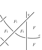
$\Longrightarrow$ 

Figure 19. A type 3 Reidemeister move

Similarly as in the proof of Theorem 4.9, we construct a filtered tree whose successive closures gradually contain $\partial F_{1}^{\prime},\partial F_{2}^{\prime}$ and $\partial F_{3}^{\prime}$ without introducing bad edges and cutting arcs. During the construction, the nonalternating edges $\overline{v_{1}v_{2}}$, $\overline{v_{3}v_{4}}$ and $\overline{v_{4}v_{5}}$ will appear as doubly good edges. We skip the detail.

6. Examples and non-examples

6.1. Examples of Theorem 4.9

The first of the three diagrams in each figure is the minimal diagram which is $(n,1)$-nonalternating. The second is obtained by a type 3 Reidemeister move over the face $F_{3}$. The third is marked with a good filtered tree whose closure has three doubly good edges. If a black-thickend edge is $\overline{ij}$ with $i<j$ then it is the $j$-th edge of the tree. This comment also applies to the subsection 6.3.

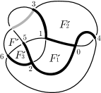
Figure 20. $(2,1)$-nonlaternating : $\alpha(8n3)=7$

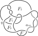
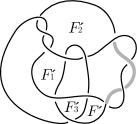
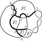
Figure 21. $(3,1)$-nonlaternating : $\alpha(12n475)=10$

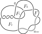
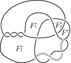
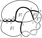
Figure 22. $(4,1)$-nonlaternating : $\alpha(12n725)=10$

6.2. Non-examples of Theorem 4.9

Each figure shows same diagram twice with different choices of faces $F_{1}$, $F_{2}$, $F_{3}$ and $F$. One can check that a condition of the theorem does not hold. This comment also applies to the subsection 6.4.

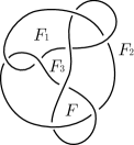
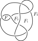
Figure 23. $(2,1)$-nonlaternating : $\alpha(8n2)=8$

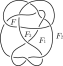
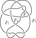
Figure 24. $(3,1)$-nonlaternating : $\alpha(12n699)=12$

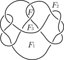
Figure 25. $(4,1)$-nonlaternating : $\alpha(12n305)=12$

6.3. Examples of Theorem 4.10

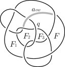
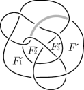
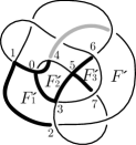
Figure 26. $2$-nonalternating : $\alpha(12n810)=11$

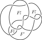
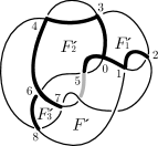
Figure 27. $3$-nonalternating : $\alpha(11n110)=10$

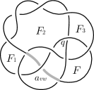
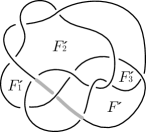
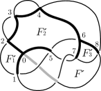
Figure 28. $4$-nonalternating : $\alpha(12n847)=11$

6.4. Non-examples of Theorem 4.10

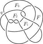
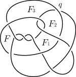
Figure 29. $2$-nonalternating : $\alpha(12n777)=12$

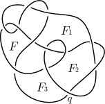
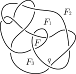
Figure 30. $3$-nonalternating : $\alpha(12n389)=12$

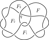
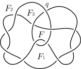
Figure 31. $4$-nonalternating : $\alpha(12n767)=12$

7. Nonalternating knots with $\alpha(K)=c(K)-1$

In [11] Nutt identified all knots up to arc index 9. In [2] Beltrami determined arc index for prime knots up to 10 crossings. In [5] Jin et al. identified all prime knots up to arc index 10. In [9] Ng determined arc index for prime knots up to 11 crossings. In [6] Jin and Park identified the prime knots up to arc index 11.

Using the Dowker-Thistlethwaite codes contained in Knotscape [14], we made lists of $13$ crossing knots and $14$ crossing knots which are $(n,1)$-nonalternating, $n$-nonlaternating or almost alternating. Applying the conditions listed in the theorems, we were able to find the lists below.

7.1. A partial list of 13 crossing knots with arc index 12

The 13 crosssing knots in the lists below do not appear in the article [7] containing all prime knots up to arc index 11. Using the methods described in the proofs of main theorems, we were able to find grid diagrams of them with 12 vertical arcs. In the grid diagrams below, we have the convention that the vertical edges pass over the horizontal edges.

$(2,1)$-nonalternating

\begin{picture}(66.0,0.0)(0.0,-15.0)\end{picture}\begin{picture}(66.0,0.0)(0.0,-15.0)\end{picture}\begin{picture}(66.0,0.0)(0.0,-15.0)\end{picture}\begin{picture}(66.0,0.0)(0.0,-15.0)\end{picture}

$(3,1)$-nonalternating

\begin{picture}(66.0,0.0)(0.0,-15.0)\end{picture}

$2$-nonalternating

\begin{picture}(66.0,75.0)(0.0,-15.0)\end{picture}\begin{picture}(66.0,75.0)(0.0,-15.0)\end{picture}\begin{picture}(66.0,0.0)(0.0,-15.0)\end{picture}\begin{picture}(66.0,0.0)(0.0,-15.0)\end{picture}\begin{picture}(66.0,0.0)(0.0,-15.0)\end{picture}\begin{picture}(66.0,0.0)(0.0,-15.0)\end{picture}

$3$-nonalternating

\begin{picture}(66.0,0.0)(0.0,-15.0)\end{picture}\begin{picture}(66.0,0.0)(0.0,-15.0)\end{picture}\begin{picture}(66.0,0.0)(0.0,-15.0)\end{picture}\begin{picture}(66.0,0.0)(0.0,-15.0)\end{picture}

$4$-nonalternating

\begin{picture}(66.0,0.0)(0.0,-15.0)\end{picture}\begin{picture}(66.0,0.0)(0.0,-15.0)\end{picture}\begin{picture}(66.0,0.0)(0.0,-15.0)\end{picture}

$5$-nonalternating

\begin{picture}(66.0,0.0)(0.0,-15.0)\end{picture}\begin{picture}(66.0,0.0)(0.0,-15.0)\end{picture}\begin{picture}(66.0,0.0)(0.0,-15.0)\end{picture}\begin{picture}(66.0,0.0)(0.0,-15.0)\end{picture}\begin{picture}(66.0,0.0)(0.0,-15.0)\end{picture}

Almost alternating

\begin{picture}(66.0,0.0)(0.0,-15.0)\end{picture}

7.2. A partial list of 14 crossing knots with arc index 13

The 14 crosssing knots in the lists below have Kauffman $v$-spread equal to 11, hence their arc index is at least 13. Using the methods described in the proofs of main theorems, we were able to find grid diagrams of them with 13 vertical arcs.

$(2,1)$-nonalternating

$(3,1)$-nonalternating

$(4,1)$-nonalternating

$(5,1)$-nonalternating

$2$-nonalternating

$3$-nonalternating

$4$-nonalternating

$6$-nonalternating

Almost alternating

References

- [1] Yongju Bae and Chan-Young Park, An upper bound of arc index of links, Math. Proc. Camb. Phil. Soc. 129 (2000) 491–500.
- [2] Elisabeta Beltrami, Arc index of non-alternating links, J. Knot Theory Ramifications. 11(3) (2002) 431–444.
- [3] Peter R. Cromwell, Embedding knots and links in an open book I: Basic properties, Topology Appl. 64 (1995) 37–58.
- [4] Peter R. Cromwell and Ian J. Nutt, Embedding knots and links in an open book II. Bounds on arc index, Math. Proc. Camb. Phil. Soc. 119 (1996), 309–319.
- [5] Gyo Taek Jin, Hun Kim, Gye-Seon Lee, Jae Ho Gong, Hyuntae Kim, Hyunwoo Kim and Seul Ah Oh, Prime knots with arc index up to 10, Intelligence of Low Dimensional Topology 2006, Series on Knots and Everything Book vol. 40, World Scientific Publishing Co., 65–74, 2006.
- [6] Gyo Taek Jin and Wang Keun Park, Prime knots with arc index up to 11 and an upper bound of arc index for non-alternating knots, J. Knot Theory Ramifications, 19(12) (2010) 1655–1672.
- [7] Gyo Taek Jin and Wang Keun Park, A tabulation of prime knots up to arc index 11, J. Knot Theory Ramifications, to appear.
- [8] H. R. Morton and E. Beltrami, Arc index and the Kauffman polynomial, Math. Proc. Camb. Phil. Soc. 123 (1998) 41–48.
- [9] Lenhard Ng, On arc index and maximal Thurston-Bennequin number, arXiv: math/0612356
- [10] Ian J. Nutt, Arc index and Kauffman polynomial, J. Knot Theory Ramifications. 6(1) (1997) 61–77.
- [11] Ian J. Nutt, Embedding knots and links in an open book III. On the braid index of satellite links, Math. Proc. Camb. Phil. Soc. 126 (1999) 77–98.
- [12] Dale Rolfsen, Knots and Links, AMS Chelsea Publishing, 2003
- [13] Knotplot, http://knotplot.com/
- [14] Knotscape, http://www.math.utk.edu/morwen/knotscape.html
- [15] Table of Knot Invariants, http://www.indiana.edu/knotinfo/