On a new parameter to estimate the helium content in old stellar systems

Abstract

We introduce a new parameter $\Delta\xi$—the difference in magnitude between the red giant branch (RGB) bump and the point on the main sequence (MS) at the same color as the bump (which we call the “benchmark”)—to estimate the helium content in old stellar systems. The $\Delta\xi$ parameter is a helium indicator since an increase in helium makes, at fixed age and iron abundance, the RGB bump brighter and the MS benchmark fainter. Moreover, its sensitivity to helium is linear over the entire metallicity range. $\Delta\xi$ is also minimally affected by changes of a few Gyr in cluster age, by uncertainties in the photometric zero-point, by the amount of reddening, or by the effects of evolution on the horizontal branch. The two main drawbacks of the $\Delta\xi$ parameter include the need for precise and large photometric data sets from the RGB bump down to the MS benchmark, and a strong dependence of the $\Delta\hbox{\rm Y}/\Delta\xi$ slope on metallicity. To provide an empirical basis for the $\Delta\xi$ parameter we selected almost two dozen relatively bright Galactic Globular Clusters (GGCs) with low foreground reddening, and a broad range of iron abundance ($-2.45\leq$[Fe/H]$\leq-0.70$ dex). Moreover, the selected GGCs have precise, relatively deep, and homogeneous multi-band (BVI) photometry. We found that the observed $\Delta\xi$ parameters and those predicted from $\alpha$-enhanced evolutionary models agree reasonably well if we assume a primordial helium content of Y=0.20 (abundance by mass). The discrepancy in the photometric $B$ band becomes of the order of 4$\sigma$ ($\Delta B=0.20$ mag) only in the metal-poor regime. Comparison with evolutionary prescriptions based on a canonical primordial helium content (Y=0.245, $\Delta$Y/$\Delta$Z [helium-to-metal enrichment ratio]=1.4) indicates that the observed $\Delta\xi$ values are systematically smaller than predicted. This discrepancy ranges from 5$\sigma$ ($\Delta B=0.26$ mag) in the metal-rich regime to 10$\sigma$ ($\Delta B=0.51$ mag) in the metal-poor regime. The outcome is the same if predicted $\Delta\xi$ parameters are based on evolutionary models with CNO enhancements in addition to $\alpha$ enhancements. The discrepancy becomes even larger if we extend the comparison to He-enhanced models. These findings support previous results (Meissner & Weiss 2006, A&A, 456, 1085; Di Cecco et al. 2010, ApJ, 712, 527; Cassisi et al. 2011, A&A, 527, A59) suggesting that current stellar evolutionary models overestimate the luminosity of the RGB bump. We also found that including envelope overshooting can eliminate the discrepancy, as originally suggested by Alongi et al. (1993, A&AS, 97, 851); atomic diffusion and mass loss play smaller roles. The $\Delta\xi$ parameter of GGCs, in spite of the possible limitations concerning the input physics of current evolutionary models, provides an independent detection of pre-stellar helium at least at the 5$\sigma$ level.

1 Introduction

The notion of possible variations in helium abundance between different Globular Clusters (GCs) dates back more than forty years (van den Bergh, 1967), in connection with the second parameter phenomenon (VandenBerg, 2000; Recio-Blanco et al., 2006). Recently, the possibility of different helium abundances among stars within individual GCs has also been suggested to explain not only the presence of multiple clumps and extended blue tails on the horizontal branch, but also multiple parallel main sequences and subgiant branches (D’Antona & Caloi, 2008, and references therein). This working hypothesis relies on the well established anti-correlations between the molecular band-strengths of CN and CH (Smith, 1987; Kraft, 1994) and between O–Na and Mg–Al measured in both evolved (red giant [RG] and horizontal branch [HB]) and unevolved (main sequence [MS]) stars of GCs investigated with high-resolution spectroscopy (Pilachowski, Sneden & Wallerstein, 1983; Ramirez & Cohen, 2002; Gratton, Sneden & Carretta, 2004). Furthermore, deep Hubble Space Telescope photometry has disclosed the presence of multiple stellar populations in several massive GCs. Together with the long-known case of $\omega$ Centauri (Anderson, 2002; Bedin et al., 2004), parallel stellar sequences have now been detected in a number of GCs: NGC 2808 (D’Antona et al., 2005; Piotto et al., 2007), M54 (Siegel et al., 2007) and NGC 1851 (Calamida et al., 2007; Milone et al., 2008). In some of these cases the multiple sequences might be explained by sub-populations differing either in He abundance (Norris, 2004; D’Antona et al., 2005; D’Antona & Caloi, 2008; Piotto et al., 2007), or in CNO abundance.

We still lack a direct detection of helium variations among the sub-populations in a GC, because helium absorption lines in the visible spectral region appear only at effective temperatures hotter than 10,000 K (Behr, 2003a, b; Moehler et al., 2004). Such high temperatures in a GC are typical of hot and extreme HB stars but, unfortunately, their helium abundances cannot be adopted to constrain the original helium content because gravitational settling and/or radiative levitation can affect their surface abundances. In a recent investigation Villanova et al. (2009) identified helium absorption lines in a few warm cluster HB stars that should be weakly affected by these mechanisms, but the range in effective temperature remains very narrow.

Interestingly enough, Preston (2009) has identified both HeI and HeII emission and absorption lines in field RR Lyrae stars. The lines appear during the rising branch of the light curve and appear to be the consequence of shocks propagating through the extended atmosphere soon after the phase of minimum radius (Bono et al., 1994; Chadid & Gillet, 1996). The idea is not new and dates back at least to Wallerstein (1959), who detected helium emission lines in his seminal investigation of Type II Cepheids. The key advantage of RR Lyrae stars, when compared with similar detections of helium lines in hot and extreme HB stars (Behr, 2003b) is that they have an extensive convective envelope, and therefore they are minimally affected by gravitational settling and/or radiative levitation (Michaud et al., 2004). The drawback is that quantitative measurement of the helium abundance requires hydrodynamical atmosphere models simultaneously accounting for time-dependent convective transport and radiative transfer together with the formation and the propagation of sonic shocks.

A new approach has been suggested by Dupree et al. (2011), who detected the chromospheric HeI line at 10830 Å in a few RG stars having similar magnitudes and colors in $\omega$ Cen. The He line was detected in more metal-rich stars and it seems to be correlated with Al and Na, but no clear correlation was found with Fe abundance. However, a more detailed non-LTE analysis of the absolute abundance of He is required before firm conclusions can be drawn concerning the occurrence of a spread among the different sub-populations.

To overcome the thorny problems connected with the spectroscopic measurements, Iben (1968) suggested the use of the R parameter—the ratio of the number of HB stars to the number of RGB stars brighter than the flat part of the HB—to estimate the initial He abundance of cluster stars. Two other independent constraints on the overall helium content in GCs were suggested by Caputo et al. (1983). The $\Delta$ parameter, which is the difference in magnitude between the MS at $(\hbox{\it B--V\/})_{\circ}=0.7$ and the luminosity level of the flat part of the HB, and the A parameter, which is the mass-to-luminosity ratio of RR Lyrae stars. The pros and cons of these parameters have been discussed in a thorough investigation by Sandquist (2000). Theoretical and empirical limitations affecting the precision of the R parameter have been also discussed by Zoccali et al. (2000), Riello et al. (2003), Cassisi et al. (2003) and Salaris et al. (2004).

The key feature of all three parameters is that they are directly or indirectly connected with the HB luminosity level. In spite of recent improvements in photometric precision and the increased use of a multi-wavelength approach, we still lack firm empirical methods to predict the HB luminosity level in GCs. This problem is partially due to substantial change in the HB morphology when moving from metal-poor (generally blue HB) to metal-rich (red HB) GCs. Additionally, we still lack a robust diagnostic to constrain the actual off-ZAHB evolution of HB stars (Ferraro et al., 1999; Di Cecco et al., 2010; Cassisi et al., 2011).

To overcome these longstanding problems we propose a new parameter—which we call $\Delta\xi$—to estimate the helium content of GCs. The $\Delta\xi$ parameter is the difference in magnitude between the RGB bump and a benchmark defined as the point on the (essentially unevolved) MS at the same color as the RGB bump. In the following we discuss the theoretical framework adopted and the sample of globular clusters we have selected to calibrate this new parameter.

2 Theoretical framework

To provide a quantitative theoretical framework for inferring the helium content of GCs we adopted the evolutionary models provided by Pietrinferni et al. (2004, 2006). These models were computed using a recent version of the FRANEC evolutionary code (Chieffi & Straniero, 1989). The reader interested in a detailed discussion of the adopted input physics is referred to the above papers. Here we mention only that we adopted the radiative opacity tables from the Livermore group (Iglesias & Rogers, 1996) for interior temperatures higher than $10^{4}$ K, and from Ferguson et al. (2005) for the atmospheres. Thermal conduction is accounted for following the prescriptions by Potekhin (1999). We have updated the plasma-neutrino energy loss rates according to the results provided by Haft et al. (1994). The nuclear reaction rates have been updated using the NACRE data base (Angulo et al., 1999), with the exception of the ${}^{12}C$($\alpha$;$\gamma$)${}^{16}O$ reaction; for this reaction, we adopted the recent determination by Kunz et al. (2002). We also adopted the equation of state (EOS) provided by A. Irwin.

The adopted $\alpha$-enhanced mixture follows the prescriptions by Salaris et al. (1997) and by Salaris & Weiss (1998), with a Solar iron content of 0.0198 from Grevesse & Noels (1993), a primordial helium content of Y=0.245 (Cassisi et al., 2003), and a helium-to-metal enrichment of $\Delta\hbox{\rm Y}/\Delta\hbox{\rm Z}$=1.4 (Pietrinferni et al., 2004). The cluster isochrones were transformed into the observational plane using the bolometric corrections (BCs) and the color-temperature relations (CTRs) provided by Castelli & Kurucz (2003).

Note that together with the $\alpha$-enhanced models, we also considered cluster isochrones constructed assuming CNO-Na abundance anti-correlations (Pietrinferni et al., 2009). These sets of isochrones have the advantage of having been constructed for the same iron abundances as the $\alpha$-enhanced models. The heavy-element mixture adopted in these evolutionary models is defined as extreme (see Table 1 in Pietrinferni et al., 2009), and when compared with the canonical $\alpha$-enhanced mixture includes an increase in N and Na abundance of 1.8 and 0.8 dex and a decrease in C and O abundance of 0.6 and 0.8 dex, respectively. We did not include the anti-correlation between Mg and Al, since its impact on evolutionary models is negligible (Salaris et al., 2006). The transformation of these evolutionary models into the observational plane does require a set of bolometric corrections (BCs) and color-temperature relations (CTRs) computed for the same mixtures; these became available only very recently (Sbordone et al., 2010). However, Pietrinferni et al. (2009) found that BCs and CTRs computed for simple $\alpha$-enhanced mixtures mimic the same behavior. Moreover, Di Cecco et al. (2010) found that BCs and CTRs hardly depend—at fixed total metallicity—on changes in the detailed mixture. The total metallicity of the atmosphere models adopted to transform the $\alpha$- and CNO-enhanced models was estimated using the Salaris et al. (1993) relation with [$\alpha$/Fe]=0.62 dex.

Finally, we mention that current isochrones together with similar predictions available in the literature (VandenBerg et al., 2000; Dotter et al., 2007; Bertelli et al., 2008) give ages for GCs that are, within the errors, consistent with the WMAP age for the Universe of 13.7 Gyr (Komatsu et al., 2011; Larson et al., 2011), and provide a quite similar age ranking for the Galactic GCs (Marín-Franch et al., 2009; Cassisi et al., 2011).

3 Optical data sets

To provide a solid empirical basis for validating the $\Delta\xi$ parameter we selected a sample of relatively luminous GCs (for good statistics), covering a broad range in metallicity (–2.45$\leq$[Fe/H]$\leq$–0.70), with different structural parameters, and all having relatively low foreground reddening ($E(\hbox{\it B--V\/})\leq 0.14$, except for NGC 6352 with $E(\hbox{\it B--V\/})=0.21$ mag). Moreover and even more importantly, we selected GCs for which precise and relatively deep photometry is available in the BVI photometric bands. To reduce the possibility of any subtle errors caused by the absolute photometric calibration or by the reduction strategy, we only adopted catalogs available in the data base maintained by co-author PBS. We ended up with a sample of almost two dozen GCs; their names, reddenings, metallicities and total visual magnitudes are listed in the first four columns of Table 1. Note that the cluster iron abundances are based on the metallicity scale provided by Kraft & Ivans (2003) based on FeII lines in high-resolution spectra. For the clusters for which the Kraft & Ivans metallicity was not available we adopted the iron abundances on the metallicity scale by Carretta et al. (2009) calibrated using FeI lines in high-resolution spectra. The mean difference between the two metallicity scales is minimal ($\lesssim$0.1 dex) and vanishingly small in the metal-poor regime (see their Fig. 10).

All of these clusters have been calibrated to the Johnson-Cousins BVI photometric system of Landolt (1973, 1992) as described by Stetson (2000, 2005). In every case the corpus of observations is quite rich, ranging from a minimum of 118 (NGC 6362 in $B$) to a maximum of 3939 (NGC 6341 in $I$) individual CCD images per filter in each cluster (median: 946 images per filter per cluster). The instrumental observations have been referred to the standard system by means of local standards within each field. The GCs in our sample have calibrated data in all three of the $B$, $V$, and $I$ bands based on a minimum of 118 (NGC 6362) and a maximum of 3690 (NGC 6341) local standards (median: 972). Observations for each of the different clusters were obtained during a minimum of 7 (NGC 6541) and a maximum of 44 (NGC 6341) different observing runs (median: 16). It must be stressed, however, that since our proposed methodology relies on the difference in apparent magnitude between two stellar sequences at fixed color absolute photometric zero points are unnecessary, and possible errors in the color transformations of the photometric calibration are irrelevant (provided any such errors are unaffected by stellar surface gravity). The principal observational requirement of this work is that the photometry be consistently precise and linear over the required magnitude range. We believe that our data set, based on a very large number of individual CCD images from many different observing runs and a substantial and homogeneous body of local photometric standards for each cluster, guarantees that this requirement is met to a higher degree than in any previous photometric surveys of Milky Way GCs.

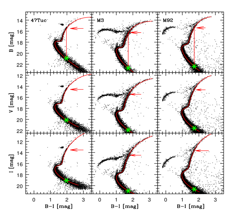
Figure 1: Top – $B$,B–I color-magnitude diagram from left to right of a metal-rich ([Fe/H] =–0.70, 47 Tuc), a metal-intermediate ([Fe/H] =–1.50, M3) and a metal-poor ([Fe/H] =–2.38, M92) GC. The red solid curves show the cluster ridge lines. The red arrows mark the position of the RGB bump, while the green asterisks show the MS benchmark. The vertical red lines show the difference in magnitude between the RGB bump and the MS benchmark. Middle – Same as the top, but in the $V$,B–I color-magnitude diagram. Bottom – Same as the top, but in the $I$,B–I color-magnitude diagram.

For each GC we estimated the ridge line in both the $V$,B–V and the $V$,V–I color-magnitude diagram (CMD). The exact approach adopted to estimate the ridge lines will be described in a future paper (Ferraro et al. 2011, in preparation). Fig. 1 shows three different CMDs for three clusters that are representative of metal-rich (47 Tuc), metal-intermediate (M3) and metal-poor (M92) GCs. The red solid curves display the ridge lines that we have estimated. The approach we adopted to estimate the magnitude and the color of the RGB bump has already been described in Di Cecco et al. (2010). The difference between the current $V$-band RGB bumps and those estimated by Di Cecco et al. (2010) is on average 0.00$\pm$0.04 mag (12 GCs). The difference compared to the RGB bumps estimated by Riello et al. (2003) is +0.01$\pm$0.07 mag (12 GCs), while the difference with the RGB bumps provided by Cassisi et al. (2011) is –0.03$\pm$0.05 mag. We performed a series of tests to estimate the accuracy of the position of the bump along the RGB using different colors (B–I, B–V, V–I) and we found that among them V–I provides the most precise measurements. We plan to provide a more detailed discussion concerning the pros and cons of both optical and near-infrared colors to estimate the $\Delta\xi$-parameter in a future paper. The $B,V$ magnitudes and the V–I colors of the RGB bumps are listed in columns 5, 6 and 7 of Table 1. The $B,V$ magnitudes of the MS benchmark having the same V–I color as the RGB bump were estimated by interpolating the ridge line (see the green asterisks plotted in Fig. 1) and they are listed in columns 8 and 9 of Table 1.

The data in Table 1 confirm the visual impression from Fig. 1 that the luminosity of the RGB bump varies inversely with the metallicity of the cluster. The $\Delta\xi$ parameter is therefore more prone to Poisson statistics and random photometric errors at the metal-poor end since in this regime the bump falls in a region of the RGB where the lifetime is shorter than at fainter magnitudes and the relative number of RG stars steadily decreases. The color of the bump also becomes redder relative to the turnoff due to the slope of the RGB, and the apparent magnitude of the MS benchmark becomes correspondingly fainter.

4 Comparison between theory and observations

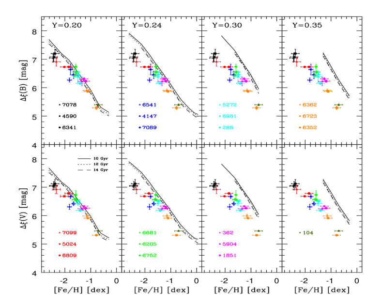
Figure 2: Top – Difference in the $B$-band magnitude between the RGB bump and the MS benchmark for the selected GCs as a function of the iron abundance. The selected GCs are marked with different symbols and colors. The dashed, dotted and solid lines display theoretical predictions for three different cluster ages (10,12,14 Gyr) according to the BASTI data base. The adopted cluster isochrones are based on evolutionary models computed assuming an $\alpha$-enhanced mixture, different iron abundances (–2.6$\lesssim$ [Fe/H] $\lesssim$ –0.3 dex) and five different He contents (Y=0.20–0.40). Predictions for Y=0.40 are not plotted, since the bump was identifiable only in a few isochrones. Bottom – Same as the top, but for the $V$-band magnitude.

We estimated the $\Delta\xi$ parameter in two different bands ($B$ and $V$); these results are listed in columns 10 and 11 of Table 1, together with their intrinsic errors, and plotted in Fig. 2. The adopted cluster isochrones were retrieved from the BASTI data base. In particular, we estimated the predicted $\Delta\xi$ parameter using cluster isochrones based on evolutionary models constructed for iron abundances covering the entire range typical of old, low-mass stars, $\alpha$-enhanced ([$\alpha$/Fe]=+0.40 dex) mixtures and a mass-loss rate à la Reimers with $\eta$=0.4. We adopted five different helium abundances, namely Y=0.20, 0.245, 0.30, 0.35 and 0.40 (relative abundance in terms of mass fraction). The models with Y=0.20, 0.30, 0.35 and 0.40 were constructed assuming a constant helium content over the entire metallicity range, while those with Y=0.245 were constructed assuming a helium-to-metal enrichment ratio $\Delta{\rm Y}/\Delta{\rm Z}\;$=1.4 (see §2). Note that the models with Y=0.20 have been specifically computed for this experiment, but they will become available at the web site mentioned above. To constrain the possible dependence on cluster age, we adopted three different values spanning the generally accepted range of GC ages, namely 10, 12, 14 Gyr (see dashed, dotted and solid lines in Fig. 2).

The predictions for Y=0.40 were not included in Fig. 2 because the bump was identifiable only in a few metal-rich compositions and for the older ages. The increase in helium causes, at fixed age and metal content, a decrease in the envelope opacity. This means that the maximum depth reached by the outer convective region during the first dredge-up becomes shallower and the discontinuity in the hydrogen profile left over by the retreating convective envelope is milder. Therefore, the H-burning shell crosses the chemical discontinuity at brighter magnitudes during faster evolutionary phases and, as a result, the bump becomes less and less evident.

The main advantages in using the $\Delta\xi$ parameter to estimate the helium content are the following: i) An increase in He content causes, at fixed cluster age and iron content, a decrease in the envelope opacity and an increase in the mean molecular weight. This means that an increase in He makes the RGB bump systematically brighter and the MS benchmark systematically fainter. The sensitivity to helium is very good, and indeed the derivatives for $\alpha$-enhanced structures, at fixed iron and age, attain values similar to the $\Delta$ parameter (see Table 2). ii) The sensitivity to age is small, and indeed the derivatives for $\alpha$-enhanced structures, at fixed iron and helium, attain minimal values. iii) There is no dependence on photometric zero-point or interstellar extinction or reddening. iv) The derivative is almost linear over the entire metallicity range (see Fig. 2). This evidence is supported by both theory and observation. The R parameter, in contrast, shows a well defined change in the slope for [Fe/H]$\approx$–0.70 dex (Zoccali et al., 2000). v) There is no dependence on HB evolutionary effects. In contrast, the R, $\Delta$, and A parameters are all affected by the off-ZAHB evolution of HB stars.

The use of the $\Delta\xi$ parameter has two main drawbacks: i) Precise, linear photometry from the RGB bump down to the MS benchmark is required for photometric data sets large enough to properly identify the RGB bump. ii) There is a definite metallicity dependence, and indeed the derivative ($\sim$1 mag/dex) is at least 0.7 dex larger than for the other helium indicators (see Table 2). The above points confirm that robust He estimates based on the $\Delta\xi$ parameter do require precise photometry and accurate spectroscopic iron abundances.

The positive features of the predicted $\Delta\xi$ parameter allow us to derive an analytical relation with iron and helium content. Using a multi-linear regression over the entire set of $\Delta\xi^{B}$- and $\Delta\xi^{V}$ parameter, we found:

$Y=-0.525\pm 0.037+0.158\pm 0.007\,\Delta\xi^{B}+0.190\pm 0.008\,\hbox{\rm[Fe/H]}\;\;\sigma=0.018$
                                                                                                                                         [1]
$Y=-0.537\pm 0.037+0.157\pm 0.007\,\Delta\xi^{V}+0.180\pm 0.008\,\hbox{\rm[Fe/H]}\;\;\sigma=0.018$

where $\sigma$ is the standard deviation and the other symbols have their usual meaning. Note that we have neglected the age dependence because the dependence on this parameter is imperceptible within the typical age range of GCs.

The above analytical relations do allow us to provide individual helium estimates for GCs. However, the comparison between theory and observation indicates that the predicted $\Delta\xi$ parameters are systematically larger than observed and the discrepancy steadily increases when moving from lower to higher helium contents. Moreover, the discrepancy, at fixed helium content, increases when moving from metal-rich to metal-poor GCs. To represent the observed, empirical values of $\Delta\xi$ as a function of metallicity, we performed linear least-squares fits to the data in Table 1 and obtained:

$\Delta\xi^{B}=4.75\pm 0.13-1.04\pm 0.08\,\hbox{\rm[Fe/H]}\;\;\sigma=0.08$ mag
                                                                                                                                         [2]
$\Delta\xi^{V}=4.85\pm 0.12-1.00\pm 0.07\,\hbox{\rm[Fe/H]}\;\;\sigma=0.09$ mag

The above fits were performed by using as weights the intrinsic errors on the $\Delta\xi$ values. The anonymous referee noted that the slope of the $\Delta\xi$ relations might not be linear over the entire metallicity range. In particular, the slope seems to become steeper in the metal-rich regime. However, this inference is based on only two GCs (NGC 6352, NGC104). Additional data in the high metallicity tail of GGCs are required to reach more quantitative conclusions. However, to constrain the impact of a possible change in the slope we performed the same fits by using only GCs more metal-poor than [Fe/H] $\leq$-1 dex. We ended up with a sample of 20 GCs and found:

$\Delta\xi^{B}=5.00\pm 0.15-0.90\pm 0.09\,\hbox{\rm[Fe/H]}\;\;\sigma=0.13$ mag
                                                                                                                                         [3]
$\Delta\xi^{V}=5.18\pm 0.13-0.81\pm 0.07\,\hbox{\rm[Fe/H]}\;\;\sigma=0.17$ mag

The new fits are characterized by slopes that are slightly shallower and zero-points that are mildly larger, but the two sets of least-squares solutions agree within 1$\sigma$.

The small intrinsic dispersions of the above empirical relations suggest that the $\Delta\xi$ parameter can be adopted to identify GCs with peculiar He abundances. The $\Delta\xi$ values listed in Table 1 and the analytical relations based on the less metal-rich GCs indicate that the possible dispersion in helium among the target GCs is minimal. We found that only two GCs—M13 and NGC 6541—show differences larger than 1.5$\sigma$ both in the $\Delta\xi^{B}$ and $\Delta\xi^{V}$ parameters. However, the discrepancy concerning NGC 6541 should be treated with caution, since it and NGC 6352 are the two GCs in our sample with the largest reddening. We are only left with M13 for which the discrepancy ranges from 1.3 to 2.6$\sigma$ in the $V$ and in the $B$ bands, respectively. By using the theoretical relations [1] we found that the quoted differences imply on average a difference in helium content, when compared with the bulk of GCs, that is of the order of 1$\sigma$ ($\Delta Y$=0.031$\pm$0.025). The lack of a clear evidence of helium enhancement in M13 soundly supports the recent results obtained by Sandquist et al. (2000) using the R parameter. Unfortunately, we cannot extend the current differential analysis concerning the helium content to more metal-rich GCs, due to the scarcity in our sample of GCs in this metallicity regime.

In this context it is also noteworthy that if the He content is the second parameter affecting the HB morphology (Suda & Fujimoto, 2006), the $\Delta\xi$ parameter should be able to prove it. At the present moment, the empirical evidence does not allow us to reach a firm conclusion. The classical couple of second parameter GCs M3 and M13 (Johnson et al., 2005)—i.e. two GCs that within the errors have the same chemical composition, but different HB morphologies— show a mild difference ($\approx$2$\sigma$) in $\Delta\xi$ ($\Delta\xi^{B}$= 6.38$\pm$0.21 [M3] vs 6.74$\pm$0.09 [M13]; $\Delta\xi^{V}$= 6.43$\pm$0.07 [M3] vs 6.73$\pm$0.15 [M13]) level. On the other hand, the other classical couple of second parameter GCs NGC 288 and NGC 362 (Bellazzini et al., 2001) do not show, within the errors, any difference. The current scenario might be confused by systematic uncertainties affecting either the chemical composition (iron, $\alpha$-enhancement, CNO-enhancement) or the cluster age which are not directly correlated with a difference in He. Clearly, the simple-minded notion that He is the second parameter is not obviously correct; other factors, which are not immediately obvious, will have to be taken into account.

The comparison between the empirical and predicted relations indicates that the discrepancy in the $B$ band for the lowest helium content (Y=0.20) is negligible in the metal-rich regime ([Fe/H] $\approx$–0.8 dex) and slightly smaller than 5$\sigma$ ($\Delta B=0.26$ mag) in the metal-poor regime ([Fe/H] $\approx$–2.2 dex). The difference in magnitude with canonical helium models ranges from $\Delta B=0.26$ (5$\sigma$, [Fe/H] $\approx$–0.8 dex) to $\Delta B=0.51$ (10$\sigma$, [Fe/H] $\approx$–2.2 dex) and becomes even larger for He-enhanced models (Y=0.30: 0.64, 0.89 mag; Y=0.35: 0.95, 1.21 mag in the metal-rich and in the metal-poor regime, respectively). The difference hardly depends on the adopted photometric band, and indeed the $V$-band difference with the lowest helium models is negligible in the metal-rich regime and equal to $\Delta V=0.20$ in the metal-poor regime (4$\sigma$, [Fe/H] $\approx$–2.2 dex). The difference with canonical helium models ranges from $\Delta V=0.25$ (5$\sigma$, [Fe/H] $\approx$–0.8 dex) to $\Delta V=0.45$ (9$\sigma$, [Fe/H] $\approx$–2.2 dex).

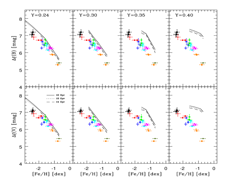
Figure 3: Same as Fig. 2, but the stellar isochrones are based on evolutionary models constructed assuming an $\alpha$- and CNO-enhanced mixture. The adopted He abundances range from Y=0.24 to Y=0.40.

The above results indicate either that the primordial helium content is roughly 20% lower than estimated using the CMB (WMAP,  Steigman, 2010) and the HII regions in metal-poor blue compact galaxies (Olive & Skillman, 2004; Izotov & Thuan, 2010; Peimbert et al., 2010) or that theory overestimates the luminosity of the RGB bump. The latter working hypothesis is also supported by recent results by Meissner & Weiss (2006) and more recently by Di Cecco et al. (2010) and by Cassisi et al. (2011). The luminosity predicted by current evolutionary models is brighter than observed in actual GCs. Note that the current discrepancy is more striking than the previous estimates, since the $\Delta\xi$ parameter is minimally affected by uncertainties in distance, age, reddening, and HB luminosity level.

To further constrain the nature of the possible culprits, we also tested the role played by possible overabundances in both $\alpha$- and CNO elements simultaneously. The comparison of the observations with predictions based on evolutionary models constructed assuming an extreme chemical mixture (see §2) is shown in Fig. 3. Note that the comparison was performed at fixed iron content, since the iron abundance is found to be constant even in GCs showing well defined anti-correlations in the lighter metals. The data plotted in this figure indicate that the impact of $\alpha$- and CNO-enhanced mixture on the current discrepancy is small.

4.1 Possible stellar modeling venues

Some crucial details of both micro- and macro-physics assumptions in the modeling of low-mass stars are far from being settled. Some of them may affect, directly or indirectly, the bump position in isochrones. Cassisi et al. (2011) already discussed a number of them (their Sect. 4.1), either estimating their impact on the bump and on the turnoff position from their own calculations or using earlier results available in the literature. Among these uncertainties atomic diffusion and convective overshooting are the most interesting ones. Here we give an example of their possible influence on evolutionary tracks in the theoretical H-R diagram for a model with $M=0.8\,M_{\odot}$ and chemical composition Z=0.001, Y=0.250. The adopted chemical composition is $\alpha$-element enhanced: it corresponds to [Fe/H] = –1.56 dex. Such a star has a turn-off age of $\approx 13$ Gyr, and therefore its RGB is quite representative for the RGB of an isochrone of this age. The evolutionary tracks were constructed using the GARSTEC code (Weiss & Schlattl, 2008), and the evolutionary models were computed with the updated ${}^{14}\mathrm{N}(p,\gamma)^{15}\mathrm{O}$ reaction (Marta et al., 2008), which was shown (Weiss et al., 2005) to increase the bump luminosity by $\approx 0.06$ mag. Note that the BASTI evolutionary tracks do not account for this reaction; its inclusion would increase the discrepancy between the predicted and the observed $\Delta\xi$ parameter by $\approx$0.15 mag.

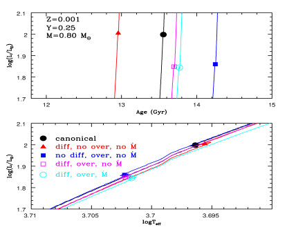
Figure 4: Top – Zoom of the evolutionary tracks around the position of the RGB bump for a model with $M=0.8\,M_{\odot}$ and chemical composition Z=0.001, Y=0.250, constructed assuming different assumptions concerning atomic diffusion, envelope overshooting and mass loss. The canonical evolutionary track (black line) neglects the above mechanisms. The position of the RGB bump is marked with different symbols. See text for more details. Bottom – Same as the top, but as a function of the logarithmic effective temperature.

We start with a canonical model without convective overshooting and neglecting atomic diffusion (black line, top panel of Fig. 4)). In this case, the bump (which is not very pronounced for these stellar parameters) is located almost exactly at log $L/L_{\odot}\,$= 2.0. The inclusion of atomic diffusion (red line) decreases—as it is well-known—the main-sequence lifetime by $\approx$0.5 Gyr, but has only a minimal impact on the bump luminosity (triangle). Indeed, it becomes slightly brighter by only $\approx$0.03 mag ($\approx$0.01 dex in $\log L$). We then included the overshooting, treated as a diffusive process as described in Weiss & Schlattl (2008), with a scale-length parameter of 0.04. The adopted value is approximately twice the value needed to fit the CMDs of open clusters (see, e.g.  Magic et al., 2010). Convective overshooting is applied at all the convective boundaries, and in particular at the lower boundary of the convective envelope. However, it is suppressed during the transient convective core phase of the pre-main sequence evolution. The blue line plotted in the top panel of Fig. 4 shows that inclusion of the envelope overshooting makes the bump (filled blue square) fainter by 0.38 mag (0.15 dex in $\log L$) when compared with the canonical evolutionary track. This is more than enough to remove the discrepancy between the predicted and observed $\Delta\xi$ parameter. Note that the difference in luminosity between the bump in the canonical evolutionary track and in the track including overshooting is causing a minimal change in effective temperature ($\Delta$ $T_{eff}\sim$65 K, see the bottom panel of Fig. 4), due to the steep slope of the RGB along these evolutionary phases. This finding confirms the results originally suggested by Alongi et al. (1993) concerning the dependence of the luminosity of the RGB bump on the envelope overshooting (see also  Cassisi et al., 2002, 2011).

As a further test, we included atomic diffusion together with envelope overshooting. The green line plotted in Fig. 4 shows that the bump (open green square) is getting even fainter, but the difference compared to the track including only the envelope overshooting is $\approx$0.05 mag (0.02 dex in $\log L$). Finally, together with envelope overshooting and atomic diffusion we also included mass loss according to the Reimers formula with the free parameter $\eta=0.6$ (cyan line). Note that this value is larger than the value typically adopted, $\eta=0.4$. However, the impact on the bump position (cyan filled circle) is negligible, the difference being of the order of a few hundredths of a magnitude.

The inclusion of diffusion and/or convective overshooting has a minimal influence on the MS benchmark, since at the effective temperature of the bump, the corresponding mass on the main sequence is hardly affected (see §4.1). Therefore, the luminosity of the MS benchmark at fixed $T_{\mathrm{eff}}$ is unaffected. This is the main difference with the results by Cassisi et al. (2011), since along the MS they adopted the turn-off as reference point. Our indicator is age-independent to a high degree of confidence. However, there is an indirect effect: the convective overshooting moves the bump downwards along the RGB, which implies a blueward change of the bump $\log T_{\mathrm{eff}}$, in this case by $+0.0055$ dex. The MS benchmark has therefore to move hotter (and brighter) on the MS by the same amount. Given the MS slope of $\triangle\log L/\triangle\log T_{\mathrm{eff}}=7.5$, this implies a luminosity increase of $\approx$0.1 mag ($\approx$10% in luminosity), thus decreasing the discrepancy between theory and observation even more. In summary, our test calculations show that reasonable assumptions concerning the convective overshooting from the bottom of the convective envelope goes in the right direction to significantly reduce the discrepancy, with the atomic diffusion playing a secondary role.

It is worth noting that the quoted numerical experiments were performed at fixed chemical composition and cluster age. This means that the possible explanation we are suggesting to remove the discrepancy between predicted and observed $\Delta\xi$ parameters needs to be tested, together with the new ${}^{14}\mathrm{N}(p,\gamma)^{15}\mathrm{O}$ reaction, in both the metal-poor and the metal-rich regime (Weiss et al. in preparation).

Finally, it is worth mentioning that Charbonnel & Zahn (2007), to explain the abundance anomalies of RGB stars, suggested the occurrence of a thermohaline instability along the RGB when the hydrogen burning shell reaches the layers with uniform chemical composition left behind by the first dredge-up. However, the occurrence of this phenomenon has a minimal impact on the luminosity of the RGB bump, since the hydrogen burning shell reaches the chemical discontinuity at earlier evolutionary phases. Moreover, recent evolutionary calculations, including state-of-the-art composition transport predictions, indicate that the thermohaline region does not reach the outer convective envelope (Wachlin et al., 2011). This limits the possibility for a non-canonical mixing process and for relevant changes in the chemical stratification above the hydrogen burning shell.

5 Conclusions and final remarks

We introduce a new $\Delta\xi$ parameter—the difference in magnitude between the RGB bump and the MS benchmark (defined as the point on the MS with the same color as the RGB bump)—to estimate the helium content of globular clusters. The advantages of the $\Delta\xi$ parameter are the following: i) An increase in He content causes, at fixed age and iron content, an RGB bump systematically brighter and an MS benchmark systematically fainter. The sensitivity to He is very good, and indeed the derivatives for $\alpha$-enhanced structures, at fixed iron and age, attain values (6.47–6.56 mag) similar to the $\Delta$ parameter (6.63 mag). ii) It has a minimal sensitivity to age, and indeed the derivatives for $\alpha$-enhanced structures, at fixed iron and helium, are minimal (–0.03 mag/Gyr). iii) It has no dependence on uncertainties in the photometric zero-point or the amount of reddening and extinction. iv) Its sensitivity to helium is almost linear at every metal abundance. vi) It is minimally affected by evolutionary effects. In contrast, the R, $\Delta$, and A parameters are all affected by the post-ZAHB evolution of HB stars.

The $\Delta\xi$ parameter has two main drawbacks: i) Precise linear photometry from the RGB bump down to the MS benchmark is required, with large enough photometric data sets to properly characterize the RGB bump. ii) The slope of the $\Delta\xi$ versus Y relation has a strong metallicity dependence. The derivative is $\sim$–1 mag/dex/dex, i.e., a factor of 0.7 larger than the $\Delta$ parameter and $\approx$1 dex larger than the R and A parameters.

In passing we note that the $\Delta\xi$ parameter, at constant helium-to-metal enrichment ratio, can also be adopted as a metallicity indicator. The slope of the metallicity dependence is similar to the slope of the RGB bump (1 vs 0.9), but the $\Delta\xi$ parameter is minimally affected by uncertainties in cluster distance and in reddening.

We have measured the $\Delta\xi$ parameter in almost two dozen GGCs. The sample was selected according to the following criteria: homogeneous photometry; low reddening; a broad metallicity range (–2.5$\,{}^{<}_{\sim}\,$ [Fe/H] $\,{}^{<}_{\sim}\,$–0.7 dex); and a range of structural properties. We found that, at first glance, theory and observation agree quite well if we assume a primordial He content of Y=0.20, and indeed they agree reasonably well in both the metal-rich and the metal-intermediate regime. However, the observed values in the metal-poor regime are 5$\sigma$ ($\Delta$B=0.26 mag) smaller than predicted. The difference with models assuming a more canonical primordial He abundance is larger, and ranges from 5$\sigma$ ($\Delta B=0.26$ mag) in the metal-rich regime to 4$\sigma$ ($\Delta B=0.51$ mag) in the metal-poor regime. The difference becomes even larger when moving to higher He contents (such as are assumed in some current interpretations of the multiple populations found in some GCs). These results support previous evidence that current evolutionary prescriptions generally overestimate the luminosity of the RGB bump (Meissner & Weiss, 2006; Di Cecco et al., 2010; Cassisi et al., 2011).

We computed a series of alternative evolutionary tracks at fixed age ($t=13$ Gyr, M=0.80 M_⊙) and chemical composition (Z=0.001, Y=0.250) and we found that plausible assumptions concerning the treatment of the envelope overshooting can account for the discrepancy between theory and observations. The atomic diffusion and the mass loss may also play secondary roles. For a thorough discussion of the possible impact of other physical parameters the reader is referred to Cassisi et al. (2011).

The current debate concerning the primordial helium content is far from being settled. The primordial helium abundance mainly affects the third and the fourth acoustic peak of the CMB angular power spectrum. The seven years of observations by WMAP have provided an opportunity to improve the accuracy of the third peak. This means that He can be treated, for the first time, as a fitted parameter in the $\Lambda$CDM model. In particular, using a flat prior with 0.01$<$ $Y_{P}$ $<$0.8, Larson et al. (2011) found $Y_{P}$=0.28${}^{+0.14}_{-0.15}$ (see their Table 8). This confirms the existence of pre-stellar helium at least at a 2$\sigma$ level. These findings were strongly supported by Komatsu et al. (2011) who combined the seven years of WMAP data with data from small-scale CMB experiments (ACBAR, Reichardt et al. 2009; QUaD, Brown et al. 2009). They found a 3$\sigma$ detection of primordial He ($Y_{P}$=0.326$\pm$0.075 [68% CL], see their figures 10 and 11). To further constrain the primordial helium they adopted a very conservative upper limit ($Y_{P}$$<$0.3) and they found (0.23 $<$$Y_{P}$$<$0.3 68% CL). These geometric determinations of the primordial helium abundance do not by themselves rule out an initial Y value as small as 0.20.

According to the most recent calculations of state-of-the-art Big Bang Nucleosynthesis (SBBN) models the primordial helium content is Y${}_{P}\approx 0.2483\pm 0.0005$. The interested reader is referred to the comprehensive review by Steigman (2007). This value agrees quite well with helium abundance estimates based on metal-poor extragalactic HII regions, namely Y${}_{P}\approx 0.240\pm 0.006$, but the impact on these measurements of possible systematic errors is still controversial (Izotov & Thuan, 2004; Olive & Skillman, 2004; Fukugita & Kawasaki, 2006; Peimbert et al., 2007).

In light of the above findings concerning the primordial He content, we followed this path: we estimated the primordial helium content using the analytical relations given in §3 and the $\Delta\xi$ parameters listed in Table 1. We found Y${}_{P}=0.181\pm 0.014$ ($\sigma$=0.034, $\Delta\xi^{B}$) and $0.183\pm 0.014$ ($\sigma$=0.033, $\Delta\xi^{V}$). The current Y_P values were estimated as weighted means, the errors are the standard error of the mean and account for the uncertainties in the coefficients of the analytical relations, while the $\sigma$’s are the standard deviations. It is worth noting that the Y_P values we found are upper limits to the primordial helium content, since some extra helium is dredged up to the surface by the deep penetration of the convective envelope during the so-called first dredge-up phase. However, the amount of extra helium is very limited, and indeed at fixed cluster age (12 Gyr) it ranges from 0.008 ([Fe/H] =–2.62 dex, M[TO]=0.80 M_⊙) to 0.02 ([Fe/H] =–0.70 dex, M[TO]=0.90 M_⊙).

The above estimates are within 1$\sigma$ of the estimates provided by the CMB experiments, and by the analysis of lower main sequence stars (Casagrande et al., 2007), but are 2$\sigma$ from the estimates provided by the SBBN models and by the measurements of extragalactic HII regions.

We also assumed that the current evolutionary models, when moving from the metal-poor to the metal-rich regime, on average underestimate the luminosity of the $\Delta\xi$ parameter by 0.35 mag because of incomplete input physics. Therefore, we can apply—as a preliminary correction—a systematic shift of 0.35 mag to the analytical relations. Note that the coefficients of the $\Delta\xi$ parameter are of the order of 0.016, so the current shift causes an increase in helium of a few percent. Under these assumptions we found a primordial helium content of Y_P=0.236$\pm$0.014 ($\Delta\xi^{B}$) and 0.238$\pm$0.014 ($\Delta\xi^{V}$).

Consideration of the above results indicates that we still lack a convincing determination of the primordial He content based on stellar observables. However, if we trust the input physics currently adopted in evolutionary models, the existence of pre-stellar helium is established at least at the 5$\sigma$ level and increases to at least a 6$\sigma$ level, if we assume that current models underestimate the luminosity of the RGB bump by a few tenths of a magnitude.

No doubt the new and accurate CMB measurements by PLANCK (Ichikawa et al., 2008) will shed new light on the long-standing problem of the abundance of the second most abundant element in the Universe. The stellar path seems also very promising, but we still need to pave it and GAIA is a fundamental step in this direction.

Table 1: Apparent $B$- and $V$-band magnitude of the RGB bump and MS benchmark, together with the $(V-I)$ color of the bump. The reddening, the mean metallicity and the total visual magnitude for each cluster are also listed.

ID (alias)	E(B-V)	[Fe/H]	$M_{V}\tablenotemark{b}$	$B_{bump}$	$V_{bump}$	(V-I)bump	$B_{MSB}$	$V_{MSB}$	$\Delta\xi^{B}$	$\Delta\xi^{V}$
	mag	dex	mag	mag	mag	mag	mag	mag	mag	mag
NGC 7078 (M15)	$0.10$	$-2.45\pm 0.15\tablenotemark{c}$	$-9.03$	$16.07\pm 0.01$	$15.25\pm 0.02$	$1.02\pm 0.04$	$23.11\pm 0.14$	$22.29\pm 0.05$	$7.04\pm 0.14$	$7.04\pm 0.05$
NGC 4590 (M68)	$0.05$	$-2.43\pm 0.15\tablenotemark{c}$	$-7.37$	$15.95\pm 0.02$	$15.15\pm 0.01$	$1.01\pm 0.01$	$23.03\pm 0.10$	$22.20\pm 0.07$	$7.08\pm 0.10$	$7.05\pm 0.07$
NGC 6341 (M92)	$0.02$	$-2.38\pm 0.15\tablenotemark{c}$	$-8.21$	$15.40\pm 0.01$	$14.64\pm 0.02$	$0.96\pm 0.02$	$22.60\pm 0.10$	$21.76\pm 0.08$	$7.20\pm 0.10$	$7.12\pm 0.08$
NGC 7099 (M30)	$0.03$	$-2.33\pm 0.15\tablenotemark{c}$	$-7.45$	$15.52\pm 0.01$	$14.71\pm 0.01$	$0.99\pm 0.02$	$22.43\pm 0.09$	$21.63\pm 0.05$	$6.91\pm 0.09$	$6.92\pm 0.05$
NGC 5024 (M53)	$0.02$	$-2.02\pm 0.15\tablenotemark{c}$	$-8.71$	$17.36\pm 0.02$	$16.61\pm 0.03$	$0.95\pm 0.18$	$24.09\pm 0.22$	$23.29\pm 0.18$	$6.73\pm 0.22$	$6.68\pm 0.18$
NGC 6809 (M55)	$0.08$	$-1.85\pm 0.15\tablenotemark{c}$	$-7.57$	$15.12\pm 0.01$	$14.17\pm 0.01$	$1.09\pm 0.01$	$21.85\pm 0.03$	$20.95\pm 0.03$	$6.73\pm 0.03$	$6.78\pm 0.03$
NGC 6541	$0.14$	$-1.82\pm 0.08\tablenotemark{d}$	$-8.52$	$15.91\pm 0.01$	$15.00\pm 0.01$	$1.08\pm 0.01$	$22.18\pm 0.07$	$21.31\pm 0.09$	$6.27\pm 0.07$	$6.31\pm 0.09$
NGC 4147	$0.02$	$-1.78\pm 0.08\tablenotemark{d}$	$-6.17$	$17.48\pm 0.01$	$16.64\pm 0.01$	$0.97\pm 0.01$	$24.12\pm 0.19$	$23.31\pm 0.07$	$6.64\pm 0.19$	$6.67\pm 0.07$
NGC 7089 (M2)	$0.06$	$-1.66\pm 0.07\tablenotemark{d}$	$-9.03$	$16.65\pm 0.01$	$15.83\pm 0.01$	$0.99\pm 0.03$	$23.10\pm 0.13$	$22.25\pm 0.07$	$6.45\pm 0.13$	$6.42\pm 0.07$
NGC 6681 (M70)	$0.07$	$-1.62\pm 0.08\tablenotemark{d}$	$-7.12$	$16.61\pm 0.01$	$15.58\pm 0.01$	$1.10\pm 0.02$	$23.04\pm 0.04$	$22.15\pm 0.04$	$6.43\pm 0.04$	$6.57\pm 0.04$
NGC 6205 (M13)	$0.02$	$-1.58\pm 0.05\tablenotemark{d}$	$-8.55$	$15.53\pm 0.01$	$14.72\pm 0.01$	$0.96\pm 0.01$	$22.27\pm 0.09$	$21.45\pm 0.15$	$6.74\pm 0.09$	$6.73\pm 0.15$
NGC 6752	$0.04$	$-1.57\pm 0.15\tablenotemark{c}$	$-7.73$	$14.49\pm 0.01$	$13.65\pm 0.01$	$1.02\pm 0.01$	$21.04\pm 0.05$	$20.20\pm 0.03$	$6.55\pm 0.05$	$6.55\pm 0.03$
NGC 5272 (M3)	$0.01$	$-1.50\pm 0.15\tablenotemark{c}$	$-8.88$	$16.25\pm 0.04$	$15.45\pm 0.02$	$0.96\pm 0.03$	$22.63\pm 0.21$	$21.88\pm 0.07$	$6.38\pm 0.21$	$6.43\pm 0.07$
NGC 6981 (M72)	$0.05$	$-1.48\pm 0.07\tablenotemark{d}$	$-7.04$	$17.57\pm 0.01$	$16.70\pm 0.01$	$1.00\pm 0.01$	$24.03\pm 0.10$	$23.20\pm 0.03$	$6.46\pm 0.10$	$6.50\pm 0.03$
NGC 288	$0.03$	$-1.41\pm 0.15\tablenotemark{c}$	$-6.75$	$16.33\pm 0.01$	$15.48\pm 0.01$	$0.96\pm 0.01$	$22.48\pm 0.03$	$21.66\pm 0.02$	$6.15\pm 0.03$	$6.18\pm 0.02$
NGC 362	$0.05$	$-1.34\pm 0.15\tablenotemark{c}$	$-8.43$	$16.25\pm 0.02$	$15.38\pm 0.01$	$0.98\pm 0.01$	$22.47\pm 0.15$	$21.62\pm 0.03$	$6.22\pm 0.15$	$6.24\pm 0.04$
NGC 5904 (M5)	$0.03$	$-1.26\pm 0.15\tablenotemark{c}$	$-8.81$	$15.82\pm 0.01$	$14.99\pm 0.01$	$0.99\pm 0.01$	$22.13\pm 0.04$	$21.32\pm 0.02$	$6.31\pm 0.04$	$6.33\pm 0.02$
NGC 1851	$0.02$	$-1.19\pm 0.15\tablenotemark{c}$	$-8.33$	$17.01\pm 0.01$	$16.13\pm 0.01$	$0.99\pm 0.01$	$23.24\pm 0.04$	$22.39\pm 0.03$	$6.23\pm 0.04$	$6.26\pm 0.03$
NGC 6362	$0.09$	$-1.15\pm 0.15\tablenotemark{c}$	$-6.95$	$16.49\pm 0.01$	$15.49\pm 0.01$	$1.06\pm 0.01$	$22.39\pm 0.05$	$21.48\pm 0.06$	$5.90\pm 0.05$	$5.99\pm 0.06$
NGC 6723	$0.05$	$-1.11\pm 0.15\tablenotemark{c}$	$-7.83$	$16.48\pm 0.01$	$15.58\pm 0.01$	$1.05\pm 0.01$	$22.35\pm 0.04$	$21.49\pm 0.03$	$5.87\pm 0.04$	$5.91\pm 0.03$
NGC 6352	$0.21$	$-0.78\pm 0.15\tablenotemark{c}$	$-6.47$	$16.90\pm 0.01$	$15.75\pm 0.01$	$1.31\pm 0.01$	$22.19\pm 0.06$	$21.06\pm 0.03$	$5.29\pm 0.06$	$5.31\pm 0.03$
NGC 104 (47Tuc)	$0.04$	$-0.70\pm 0.15\tablenotemark{c}$	$-9.42$	$15.51\pm 0.01$	$14.57\pm 0.01$	$1.03\pm 0.01$	$20.91\pm 0.03$	$20.03\pm 0.02$	$5.40\pm 0.03$	$5.46\pm 0.02$

Table 2: Derivative as a function of iron, helium and cluster age for the most popular parameters adopted to estimate the helium content in GCs.

Derivative	$\Delta\xi^{B}_{\alpha}$	$\Delta\xi^{V}_{\alpha}$	$\Delta\xi^{B}_{\alpha,CNO}$	$\Delta\xi^{V}_{\alpha,CNO}$	$R$	$\Delta$	$A$
$\left(\frac{\partial}{\partial Y}\right)^{a}_{[Fe/H]=-1.3,t=12}$	$6.47$	$6.56$	$5.07$	$5.11$	11.43	6.63	1.50
$\left(\frac{\partial}{\partial[Fe/H]}\right)^{b}_{Y=0.246,t=12}$	$-1.08$	$-1.03$	$-1.04$	$-1.00$	-0.08	-0.37	-0.05
$\left(\frac{\partial}{\partial t}\right)^{c}_{[Fe/H]=-1.3,Y=0.246}$	$-0.03$	$-0.03$	$-0.04$	$-0.04$	…	…	…

References

- Alongi et al. (1993) Alongi, M., Bertelli, G., Bressan, A., Chiosi, C., Fagotto, F., Greggio, L., & Nasi, E. 1993, A&AS, 97, 851
- Anderson (2002) Anderson, J. 2002, in Omega Centauri, A Unique Window into Astrophysics, eds. F. van Leeuwen, J. D. Hughes & G. Piotto (San Francisco, ASP), 87
- Angulo et al. (1999) Angulo, C., et al. 1999, Nuclear Physics A, 656, 3
- Bedin et al. (2004) Bedin, L. R. et al. 2004, ApJ, 605, 125
- Behr (2003a) Behr, B. 2003, ApJS, 149, 67
- Behr (2003b) Behr, B. B. 2003, ApJS, 149, 101
- Bellazzini et al. (2001) Bellazzini, M., Fusi Pecci, F. Ferraro, F. R., Galleti, S. Catelan, M., & Landsman, W. B. 2001, AJ, 122, 2569
- Bertelli et al. (2008) Bertelli, G., Girardi, L., Marigo, P., & Nasi, E. 2008, A&A, 484, 815
- Bono et al. (1994) Bono, G., Caputo, F., & Stellingwerf, R. F. 1994, ApJ, 432, L51
- Brown et al. (2009) Brown, M. L., et al. 2009, ApJ, 705, 978
- Calamida et al. (2007) Calamida, A., Bono, G., Stetson, P. B. et al. 2007, ApJ, 670, 400
- Caputo et al. (1983) Caputo, F., Cayrel, R., & Cayrel de Strobel, G. 1983, A&A, 123, 135
- Carretta et al. (2009) Carretta, E., Bragaglia, A., Gratton, R., D’Orazi, V., & Lucatello, S. 2009, A&A, 508, 695
- Casagrande et al. (2007) Casagrande, L., Flynn, C., Portinari, L., Girardi, L., & Jimenez, R. 2007, MNRAS, 382, 1516
- Cassisi et al. (2002) Cassisi, S., Salaris, M., & Bono, G. 2002, ApJ, 565, 1231
- Cassisi et al. (2003) Cassisi, S., Salaris, M., & Irwin, A. W. 2003, ApJ, 588, 862
- Cassisi et al. (2008) Cassisi, S., Salaris, M., Pietrinferni, A. et al. 2008, ApJ, 672, L115
- Cassisi et al. (2011) Cassisi, S., Marín-Franch, A., Salaris, M., Aparicio, A., Monelli, M., & Pietrinferni, A. 2011, A&A, 527, A59
- Castelli & Kurucz (2003) Castelli, F., & Kurucz, R. L. 2003, in IAU Symp. 210, Modelling of Stellar Atmospheres, eds. N. Piskunov, W.W. Weiss, D.F. Gray (San Francisco, ASP), 20
- Chadid & Gillet (1996) Chadid, M., & Gillet, D. 1996, A&A, 308, 481
- Charbonnel & Zahn (2007) Charbonnel, C., & Zahn, J.-P. 2007, A&A, 467, L15
- Chieffi & Straniero (1989) Chieffi, A., & Straniero, O. 1989, ApJS, 71, 47
- D’Antona et al. (2005) D’Antona, F., Bellazzini, M., Caloi, V., Pecci, F. F., Galleti, S., & Rood, R. T. 2005, ApJ, 631, 868
- D’Antona & Caloi (2008) D’Antona, F. & Caloi, V. 2008, MNRAS, 390, 693
- Di Cecco et al. (2010) Di Cecco, A., et al. 2010, ApJ, 712, 527
- Dotter et al. (2007) Dotter, A., Chaboyer, B., Jevremović, D., Baron, E., Ferguson, J. W., Sarajedini, A., & Anderson, J. 2007, AJ, 134, 376
- Dupree et al. (2011) Dupree, A., Smith, G. H., & Strader, J. 2011, ApJ, 728, 155
- Ferguson et al. (2005) Ferguson, J.W., Alexander, D. R., Allard, F., Barman, T., Bodnarik, J.G., Hauschildt, P.H., Heffner-Wong, A., & Tamanai, A. 2005, ApJ, 623, 585
- Ferraro et al. (1999) Ferraro, F. R., Messineo, M., Fusi Pecci, F., de Palo, M. A., Straniero, O., Chieffi, A., & Limongi, M. 1999, AJ, 118, 1738
- Fukugita & Kawasaki (2006) Fukugita, M., & Kawasaki, M. 2006, ApJ, 646, 691
- Gratton, Sneden & Carretta (2004) Gratton, R., Sneden, C., & Carretta, E. 2004, A&A, 42, 385
- Grevesse & Noels (1993) Grevesse, N., & Noels, A. 1993, Physica Scripta Volume T, 47, 133
- Haft et al. (1994) Haft, M., Raffelt, G., & Weiss, A. 1994, ApJ, 425, 222
- Harris 1996 (2010 edition) Harris, W. E. 1996, AJ, 112, 1487
- Iben (1968) Iben, I. 1968, Nature, 220, 143
- Ichikawa et al. (2008) Ichikawa, K., Sekiguchi, T., & Takahashi, T. 2008, Phys. Rev. D, 78, 043509
- Iglesias & Rogers (1996) Iglesias, C. A., & Rogers, F. J. 1996, ApJ, 464, 943
- Izotov & Thuan (2004) Izotov, Y. I., & Thuan, T. X. 2004, ApJ, 602, 200
- Izotov & Thuan (2010) Izotov, Y. I. & Thuan, T. X. 2010, ApJ, 710, L67
- Johnson et al. (2005) Johnson, C. I., Kraft, R. P., Pilachowski, C. A., Sneden, C., Ivans, I. I., Benman, G. 2005, PASP, 117, 1308
- Komatsu et al. (2011) Komatsu, E., et al. 2011, ApJS, 192, 18
- Kraft (1994) Kraft, R. P. 1994, PASP, 106, 553
- Kraft & Ivans (2003) Kraft, R. P., & Ivans, I. I. 2003, PASP, 115, 143
- Kraft & Ivans (2004) Kraft, R. P., & Ivans, I. I. 2004, in Origin and Evolution of the Elements, ed. A. McWilliam & M. Rauch, Carnegie Observatories Astrophysics Series, 33
- Kunz et al. (2002) Kunz, R., Fey, M., Jaeger, M., Mayer, A., Hammer, J. W., Staudt, G., Harissopulos, S., & Paradellis, T. 2002, ApJ, 567, 643
- Landolt (1973) Landolt, A. U. 1973, AJ, 78, 959
- Landolt (1992) Landolt, A. U. 1992, AJ, 104, 340
- Larson et al. (2011) Larson, D., et al. 2011, ApJS, 192, 16
- Magic et al. (2010) Magic, Z., Serenelli, A., Weiss, A., & Chaboyer, B. 2010, ApJ, 718, 1378
- Marín-Franch et al. (2009) Marín-Franch, A., et al. 2009, ApJ, 694, 1498
- Marta et al. (2008) Marta, M., et al. 2008, Phys. Rev. C, 78, 022802
- Meissner & Weiss (2006) Meissner, F. & Weiss, A. 2006, A&A, 456, 1085
- Michaud et al. (2004) Michaud, G., Richard, O., Richer, J., & VandenBerg, D. A. 2004, ApJ, 606, 452
- Milone et al. (2008) Milone, A. P., Bedin, L. R., Piotto, G. et al. 2008, ApJ, 673, 241
- Moehler et al. (2004) Moehler, S., Koester, D., Zoccali, M., Ferraro, F. R., Heber, U., Napiwotzki, R., & Renzini, A. 2004, A&A, 420, 515
- Norris (2004) Norris, J. E. 2004, ApJ, 612, 25
- Ochsenbein, Bauer, & Marcout (2000) Ochsenbein, F., Bauer, P., Marcout, J. 2000, A&AS, 143, 23O
- Olive & Skillman (2004) Olive, K. A., & Skillman, E. D. 2004, ApJ, 617, 29
- Peimbert et al. (2007) Peimbert, M., Luridiana, V., & Peimbert, A. 2007, ApJ, 666, 636
- Peimbert et al. (2010) Peimbert, M., Peimbert, A., Carigi, L., & Luridiana, V. 2010, IAU Symp. 268, Light Elements in the Universe, 91
- Pietrinferni et al. (2004) Pietrinferni, A., Cassisi, S., Salaris, M., & Castelli, F. 2004, ApJ, 612, 168
- Pietrinferni et al. (2006) Pietrinferni, A., Cassisi, S., Salaris, M., & Castelli, F. 2006, ApJ, 642, 797
- Pietrinferni et al. (2009) Pietrinferni, A., Cassisi, S., Salaris, M., Percival, S., & Ferguson, J. W. 2009, ApJ, 697, 275
- Pilachowski, Sneden & Wallerstein (1983) Pilachowski, C. A., Sneden, C., & Wallerstein, G. 1983, ApJS, 52, 241
- Piotto et al. (2007) Piotto, G. et al. 2007, ApJ, 661, 53
- Potekhin (1999) Potekhin, A. Y. 1999, A&A, 351, 787
- Preston (2009) Preston, G. W. 2009, A&A, 507, 1621
- Ramirez & Cohen (2002) Ramirez, S. V., & Cohen, J. G. 2002, AJ, 123, 3277
- Recio-Blanco et al. (2006) Recio-Blanco, A., Aparicio, A., Piotto, G., de Angeli, F., & Djorgovski, S. G. 2006, A&A, 452, 875
- Reichardt et al. (2009) Reichardt, C. L., et al. 2009, ApJ, 694, 1200
- Riello et al. (2003) Riello, M., et al. 2003, A&A, 410, 553
- Salaris et al. (1993) Salaris, M., Chieffi, A., & Straniero, O. 1993, ApJ, 414, 580
- Salaris et al. (1997) Salaris, M., degl’Innocenti, S., & Weiss, A. 1997, ApJ, 479, 665
- Salaris & Weiss (1998) Salaris, M., & Weiss, A. 1998, A&A, 335, 943
- Salaris et al. (2004) Salaris, M., Riello, M., Cassisi, S., & Piotto, G. 2004, A&A, 420, 911
- Salaris et al. (2006) Salaris, M., Weiss, A., Ferguson, J. W., & Fusilier, D. J. 2006, ApJ, 645, 1131
- Sandquist (2000) Sandquist, E. L. 2000, MNRAS, 313, 571
- Sandquist et al. (2000) Sandquist, E. L. Gordon, M., Levine, D. & Bolte, M. 2010, AJ, 139, 2374
- Sbordone et al. (2010) Sbordone, L., Salaris, M., Weiss, A., Cassisi, S. 2011, A&A, accepted, arXiv:1103.5863
- Siegel et al. (2007) Siegel, M. H., et al. 2007, ApJ, 667, L57
- Smith (1987) Smith, G. H. 1987, PASP, 99, 67l
- Steigman (2007) Steigman, G. 2007, Annual Review of Nuclear and Particle Science, 57, 463
- Steigman (2010) Steigman, G. 2010, JCAP, 4, 29
- Stetson (2000) Stetson, P. B. 2000, PASP, 112, 925
- Stetson (2005) Stetson, P. B. 2005, PASP, 117, 563
- Suda & Fujimoto (2006) Suda, T., & Fujimoto, M. Y. 2006, ApJ, 643, 897
- VandenBerg (2000) VandenBerg, D. A. 2000, ApJS, 129, 315
- VandenBerg et al. (2000) VandenBerg, D. A., Swenson, F. J., Rogers, F. J., Iglesias, C. A., & Alexander, D. R. 2000, ApJ, 532, 430
- van den Bergh (1967) van den Bergh, S. 1967, PASP, 79, 460
- Villanova et al. (2009) Villanova, S., Piotto, G., & Gratton, R. G. 2009, A&A, 499, 755
- Wachlin et al. (2011) Wachlin, F. C., Miller Bertolami, M. M., Althaus, L. G. 2011, A&A, submitted, arXiv1104.0832
- Wallerstein (1959) Wallerstein, G. 1959, ApJ, 130, 560
- Weiss et al. (2005) Weiss, A., Serenelli, A., Kitsikis, A., Schlattl, H., & Christensen-Dalsgaard, J. 2005, A&A, 441, 1129
- Weiss & Schlattl (2008) Weiss, A., & Schlattl, H. 2008, Ap&SS, 316, 99
- Zoccali et al. (2000) Zoccali, M., Cassisi, S., Bono, G., Piotto, G., Rich, R. M., & Djorgovski, S. G. 2000, ApJ, 538, 289