Anisotropic Inverse Cascade toward Zonal Flow in Magnetically Confined Plasmas

Abstract

We propose a new mechanism for the generation of zonal flows in magnetically confined plasmas, complementing previous theories based on a modulational instability. We derive a new conservation law that operates in the regime of weakly nonlinear dynamics, and show that it serves to focus the inverse cascade of turbulent drift wave energy into zonal flows. This mechanism continues to operate in the absence of the separation of dynamical scales typically assumed in instability calculations.

Zonal flows refer to a class of highly anisotropic flows that emerge spontaneously in response to nominally rather weakly anisotropic trends in the environment. Examples in geophysical fluids include strongly sheared east-west jets in planetary atmospheres (Jupiter, in particular). North-south variation of the Coriolis parameter provides an obvious underlying anisotropy, but is far too weak to directly explain the observed flow patterns.

Similar flows are believed to exist in magnetically confined quasi-neutral plasmas, e.g., tokamaks DIIH2005 , responding in this case to gradients in the magnetic field, background ion concentration, plasma temperature, etc. Zonal flows take on added importance in plasmas because they are believed to provide transport barriers, leading to the low to high confinement (L-H) transition, and hence may aid the goal of controlled fusion.

There have been many calculations elucidating conditions under which small-scale drift wave turbulence can produce a modulational instability, leading to exponential growth of a zonal flow pattern DRHMFS1998 ; SDS2000 ; KWPSSS2005 ; KST2010 ; CNNQ2010 . The calculations typically assume a large separation of scales, enabling a simple description of the growth of an existing zonal flow, pumped by sufficiently strong resonant small scale fluctuations. Broader conditions can probably be formulated in terms of the shape of the drift wave spectrum CNNQ2010 .

The goal here is to show that energy transfer from small scale turbulence to large scale zonal flow is a general physical phenomenon in plasmas, operating irrespective of whether the dominant interactions are local or nonlocal in scale. We derive a new “extra” conservation law, on top of those for energy and momentum/enstrophy. The inverse cascade of wave energy follows from standard arguments involving balance of energy and enstrophy flux in the spectral domain Z1992 . The extra invariant places further constraints on the energy flux, forcing it more and more strongly into the zonal wavevector sector with increasing scale. This provides a general mechanism for the observed amplification of zonal anisotropy, and will be demonstrated quantitatively through analysis of a corresponding spectral function $\phi_{\bf k}$.

A similar invariant exists in the quasigeostrophic (or CHM CHM ) equation BNZ1991 ; B1991 , and in the shallow water system BHW2011 of geophysical fluid dynamics. However, the plasma system is significantly more complicated, producing, for example, in addition to the usual CHM “vector” nonlinearity, a “scalar” nonlinearity KWPSSS2005 ; NC1995 ; OPSSS2004 ; MHM . We find it unlikely, for example, that the generalized Hasegawa-Mima (GHM) NC1995 equation (with both nonlinearities) possesses an extra invariant—this issue will be discussed further below. Given the added levels of approximation entering such reduced equations, we base our derivation directly on the more general effective two-dimensional hydrodynamic equations from which they are derived. We account for (smooth, large scale) inhomogeneity in the electron temperature (which leads to the scalar nonlinearity), applied magnetic field $B$, fluid pressure $P$, and background ion density $n_{0}$, all on the same footing. Furthermore, we do not assume any particular common direction of variation of these parameters (e.g., the “radial” direction in a tokamak foot:direction ). A single direction $\hat{\bm{\gamma}}$ emerges naturally, namely the local gradient of the ratio $n_{0}/B$, with zonal direction orthogonal to it.

The effective two-dimensional hydrodynamic equations for a magnetically confined plasma, in the $xy$-plane normal to the applied magnetic field ${\bf B}=B{\bf\hat{z}}$, are

$$\partial_{t}{\bf v}+({\bf v}\cdot\nabla){\bf v}+f{\bf\hat{z}}\times{\bf v} = -\nabla\Phi$$

$$\partial_{t}n+\nabla\cdot(n{\bf v}) = 0,$$ (1)

where $n$ is the ion number density and ${\bf v}=(v_{x},v_{y})$ the velocity. The ion cyclotron frequency is $f=q_{i}B/m_{i}$, where $q_{i},m_{i}$ are the ion charge and mass. The potential $\Phi=(q_{i}/m_{i})\varphi+W(n)$ consists an electric potential $\varphi$ (with ${\bf E}=-\nabla\varphi$), and an ion pressure term ($W$ being the solution of $m_{i}nW^{\prime}(n)=P^{\prime}(n)$, with pressure $P$ assumed a function of the density alone). Electrons move rapidly along the magnetic field lines, and are assumed to be in local equilibrium at a temperature $T$. The density then follows the Boltzmann distribution, $n=n_{0}e^{e\varphi/T}$ (so $n_{0}$ is the ion concentration when $\varphi\equiv 0$). The fluctuation contribution to ${\bf B}$ from currents generated by ${\bf v}$ is assumed small compared to $B$, and is neglected.

We will see that the slow drift wave modes in (1) are weakly coupled to all other motions, and hence support a separate set of approximate conservation laws. Most importantly, the drift wave dispersion law, essentially uniquely, admits the new conservation law BF1998 .

Irrespective of the relation between $\Phi$ and $n$ (if any), (1) leads to convective conservation of potential vorticity

$$(\partial_{t}+{\bf v}\cdot\nabla)Q=0,\ \ Q\equiv(\zeta+f)/n,$$ (2)

where $\zeta=\nabla\times{\bf v}\equiv\partial_{x}v_{y}-\partial_{y}v_{x}$ is the vorticity. In the weakly nonlinear limit one may approximate $Q\approx({\cal Q}+f)/n_{0}$, where ${\cal Q}=\zeta-fh$ and $h=(n-n_{0})/n_{0}$. From (1) one obtains the (exact) equation of motion

$$\partial_{t}{\cal Q}+\nabla\cdot({\cal Q}{\bf v})=f(1+h){\bm{\gamma}}\cdot{\bf v},\ \ {\bm{\gamma}}\equiv\nabla\ln(n_{0}/f).$$ (3)

Equation (2) gives rise to the usual infinite hierarchy of conserved integrals. We derive here an invariant of a different type. It is quadratic in ${\cal Q}$,

$$I=\frac{1}{2}\int d^{2}r_{1}\int d^{2}r_{2}X({\bf r}_{1},{\bf r}_{2}){\cal Q}({\bf r}_{1},t){\cal Q}({\bf r}_{2},t),$$ (4)

with some (symmetric) kernel $X$ to be determined. Drift wave energy and momentum may be expressed this way, but for the plasma system (1) there is an extra choice.

We utilize two small parameters. First, we assume that $n_{0},f,T$ vary slowly, namely on the scale $1/\gamma$, which itself is much larger than dominant scale $L$ of variations of the fields ${\mathcal{Q}},{\bf v}$. The quantity $\mu=\gamma L$ is the small inhomogeneity parameter. The quantities $|\nabla n_{0}|/n_{0},|\nabla f|/f,|\nabla T|/T,|\nabla{\bm{\gamma}}|/\gamma$ are all $O(\mu/L)$. This is similar to the usual beta-plane approximation in geophysical fluid dynamics, and will allow us, at a critical stage, to perform a local Fourier analysis. Second, weak nonlinearity constrains the dimensionless characteristic field amplitude $A\sim{\cal Q}/f\sim{\bf v}/fL$. The divergence term in (3) should be much smaller than the linear term on the right hand side, leading to the small nonlinearity parameter $\epsilon=A/\mu$. More generally, for a complex turbulent state, this parameter should be small on all length scales, not just the dominant scale $L$.

Using typical D-T fusion plasma parameters, $T\sim 10$ KeV, $B\sim 5$ T one obtains Larmor radius $\rho\equiv\sqrt{T/f^{2}m_{i}}\sim 3$ mm. The drift velocity is $v\approx E/B\sim\varphi/LB$, where $\varphi\approx Th/e$ is estimated from the Boltzmann relation, yielding $\zeta/f\sim h(\rho/L)^{2}$, ${\cal Q}/f\sim[1+(\rho/L)^{2}]h$, and hence $\epsilon\sim Q/fL\gamma\sim[1+(\rho/L)^{2}]h/\mu$. Using inhomogeneity scale $1/\gamma\sim 1$ m, density fluctuation scale $h\sim 10^{-2}$, and zonal flow scale $L\sim 10$ cm, one therefore obtains $\mu,\epsilon$ both of order $10^{-1}$. These are indeed small, well within the range of validity of the theory to follow.

We will prove that there are only three independent choices of the kernel $X$, for which $I$ is approximately conserved, i.e., may be considered constant over very long time scales (made more precise below). The simplest way to do so would be to bound $|\dot{I}|/I$. Unfortunately, $I$ contains oscillatory terms that have small amplitude, but whose time derivatives do not. Taking ${\bf v},{\cal Q}$ as the independent fields, we therefore consider a supplemented ZS1988 invariant

$${\cal I} = I+\int d_{12}{\cal Q}_{1}{\bf F}_{12}\cdot{\bf v}_{2}+\frac{1}{2}\int d_{123}{\cal Q}_{1}{\cal Q}_{2}{\bf M}_{123}\cdot{\bf v}_{3}$$ (5)

$$+\ \frac{1}{6}\int d_{123}Y_{123}{\cal Q}_{1}{\cal Q}_{2}{\cal Q}_{3},$$

in which, to condense the notation, numerical subscripts stand for the argument: $d_{12}=d^{2}r_{1}d^{2}r_{2}$, ${\bf v}_{2}={\bf v}({\bf r}_{2},t)$, ${\bf M}_{123}={\bf M}({\bf r}_{1},{\bf r}_{2},{\bf r}_{3})$, etc. For small $\mu,\epsilon$ the added terms will be found to be much smaller than $I$ but their time derivatives generally are not, and the kernels $X,{\bf F},{\bf M},Y$ will be determined by demanding that $|\dot{\cal I}|/f{\cal I}$ be small foot:Icorr . The kernel ${\bf M}$ is symmetric in its first two arguments, and $Y$ is symmetric in all three. Other cubic terms are possible, involving different combinations of ${\cal Q},{\bf v}$, but, due to the structure of (1), turn out not to contribute, so we drop them from the outset.

We will see that ${\bf F}_{12}=O(\mu)$, hence to compute $\dot{\cal I}$ it suffices to approximate (1), (3) by

$${\partial_{t}{\bf v}}=-f{\bf\hat{z}}\times{\bf v}-\nabla\Phi,\ \ {\partial_{t}{\mathcal{Q}}}=f{\bm{\gamma}}\cdot{\bf v}-\nabla\cdot({\mathcal{Q}}{\bf v}).$$ (6)

Here $\Phi$ depends only on the local density, and is taken to vanish for the steady state plasma. It suffices as well to use its linearized form

$$\Phi={\cal T}h=({\cal T}/f)(\zeta-{\cal Q})$$ (7)

with the slow function ${\cal T}({\bf r})=T({\bf r})/m_{i}$ in the standard cold ion limit where one neglects the pressure term.

We define for convenience the combinations

$$G_{12}=({\cal T}_{2}/f_{2})\nabla_{2}\cdot{\bf F}_{12},\ \ K_{123}=({\cal T}_{3}/f_{3})\nabla_{3}\cdot{\bf M}_{123}.$$ (8)

Using (1) and (3), integrating by parts where necessary to remove spatial derivatives from the fields, and collecting terms, one then obtains, to requisite order, $\dot{\cal I}$ with the same four terms as in (5), but with corresponding (appropriately symmetric) kernels,

$$\tilde{X}_{12} = -(G_{12}+G_{21})$$

$$\tilde{\bf F}_{12} = X_{12}f_{2}{\bm{\gamma}}_{2}+{\bf\hat{z}}\times{\bf F}_{12}f_{2}+\nabla_{2}\times G_{12}$$

$$\tilde{\bf M}_{123} = \delta_{23}\nabla_{3}X_{13}+\delta_{13}\nabla_{3}X_{23}+{\bf\hat{z}}\times{\bf M}_{123}f_{3}$$

$$+\ \nabla_{3}\times K_{123}+Y_{123}f_{3}{\bm{\gamma}}_{3}$$

$$\tilde{Y}_{123} = -(K_{123}+K_{132}+K_{321}),$$ (9)

where $\delta_{12}=\delta({\bf r}_{1}-{\bf r}_{2})$, $\nabla\times G=(\partial_{y}G,-\partial_{x}G)$, etc. A number of terms of higher order in $\mu,\epsilon$ have been dropped. These physically represent higher order nonlinearity, including interactions between drift waves and other modes contained in (1). The vanishing of $\tilde{X}_{12}$ and $\tilde{Y}_{123}$ produce the antisymmetry conditions

$$G_{12}+G_{21}=0,\ \ K_{123}+K_{132}+K_{321}=0,$$ (10)

while the vanishing of $\tilde{\bf F}_{12}$ and $\tilde{\bf M}_{12}$ produce

$${\bf F}_{12} = \frac{1}{f_{2}}\nabla_{2}G_{12}+({\bf\hat{z}}\times{\bm{\gamma}}_{2})X_{12}$$

$${\bf M}_{123} = \frac{1}{f_{3}}\nabla_{3}K_{123}+{\bf\hat{z}}\times\bigg{[}{\bm{\gamma}}_{3}Y_{123}$$ (11)

$$\left.+\frac{1}{f_{3}}\delta_{23}\nabla_{3}X_{13}+\frac{1}{f_{3}}\delta_{13}\nabla_{3}X_{23}\right].$$

Substituting (11) into the right hand sides of (9), one obtains the closed equations

$$\hat{\cal L}_{2}G_{12} = ({\bm{\gamma}}_{2}\times\nabla_{2})X_{12}$$

$$\hat{\cal L}_{3}K_{123} = ({\bm{\gamma}}_{3}\times\nabla_{3})Y_{123}-\left(\nabla_{3}\frac{\delta_{23}}{f_{3}}\right)\times(\nabla_{3}X_{13})$$ (12)

$$-\ \left(\nabla_{3}\frac{\delta_{13}}{f_{3}}\right)\times(\nabla_{3}X_{23}),$$

in which we have defined the operator

$$\hat{\cal L}=-\nabla\cdot\left(\frac{1}{f}\nabla\right)+\frac{f}{\cal T}.$$ (13)

We may write formally $G_{12}=\hat{\cal K}_{2}X_{12}$, where $\hat{\cal K}=\hat{\cal L}^{-1}({\bm{\gamma}}\times\nabla)$. Since $\hat{\cal K}_{2}$ depends only on ${\bf r}_{2}$, it does not have any particular symmetry under interchange of ${\bf r}_{1}$ and ${\bf r}_{2}$. Therefore, given that $X_{12}=X_{21}$ is symmetric, it is generally impossible to enforce antisymmetry of $G_{12}$. However, to leading order, one may ignore the ${\bf r}$ dependence of all the parameters, replacing them by constant characteristic values. In this case $\hat{\cal K}$ is translation invariant, and one seeks translation invariant solutions $X_{12}=X({\bf r}_{1}-{\bf r}_{2})$, with $X({\bf r})$ even. Hence $G_{12}=G({\bf r}_{1}-{\bf r}_{2})$ is odd, and the first of equations (10) is automatically satisfied.

Similarly, given the symmetries of $X_{12}$ and $Y_{123}$, it is impossible to enforce antisymmetry of $K_{123}$ beyond leading order. However, again replacing all parameters by constants, a consistent solution for $Y_{123}$ does exist. It is most conveniently expressed in Fourier space, where, in particular $f\hat{\cal K}\to i\Omega({\bf k})$, in which

$$\Omega=\frac{f{\bm{\gamma}}\times{\bf k}}{k^{2}+\alpha^{2}},\ \ \alpha^{2}\equiv\rho^{-2}=\frac{f^{2}}{\cal T}$$ (14)

exhibits the usual drift wave dispersion relation foot:driftwave . One obtains:

$$\hat{Y}_{123} = \frac{2A_{123}\hat{\delta}_{123}}{i(\Omega_{1}+\Omega_{2}+\Omega_{3})}\left[\left(\frac{1}{k_{3}^{2}+\alpha^{2}}-\frac{1}{k_{2}^{2}+\alpha^{2}}\right)\hat{X}_{1}\right.$$ (15)

$$+\ \left(\frac{1}{k_{1}^{2}+\alpha^{2}}-\frac{1}{k_{3}^{2}+\alpha^{2}}\right)\hat{X}_{2}$$

$$\left.+\ \left(\frac{1}{k_{2}^{2}+\alpha^{2}}-\frac{1}{k_{1}^{2}+\alpha^{2}}\right)\hat{X}_{3}\right],$$

with $\hat{\delta}_{123}=(2\pi)^{2}\delta({\bf k}_{1}+{\bf k}_{2}+{\bf k}_{3})$ reflecting translation invariance, and $A_{123}=\frac{1}{2}{\bf k}_{1}\times{\bf k}_{2}=\frac{1}{2}{\bf k}_{2}\times{\bf k}_{3}=\frac{1}{2}{\bf k}_{3}\times{\bf k}_{2}$ being the area of the resulting triangle formed by ${\bf k}_{1},{\bf k}_{2},{\bf k}_{3}$.

Up to now, $\hat{X}({\bf k})$ is arbitrary. However, (15) displays a divergence on the “three-wave resonant” surface

$${\bf k}_{1}+{\bf k}_{2}+{\bf k}_{3}=0,\ \ \Omega({\bf k}_{1})+\Omega({\bf k}_{2})+\Omega({\bf k}_{3})=0.$$ (16)

Only if the term in square brackets vanishes on this surface does a nonsingular $Y_{123}$ emerge, and this places rather stringent conditions on $X$, that we will now discuss. On this surface, the vector $f{\bf k}_{123}={\bf k}_{1}\Omega_{2}-{\bf k}_{2}\Omega_{1}={\bf k}_{2}\Omega_{3}-{\bf k}_{3}\Omega_{2}={\bf k}_{3}\Omega_{1}-{\bf k}_{1}\Omega_{3}$ is also symmetric under cyclic permutation of its indices. Defining the “zonal” and “radial” wavenumbers $p=-\hat{\bm{\gamma}}\times{\bf k}$, $q=\hat{\bm{\gamma}}\cdot{\bf k}$, one may write the term in square brackets as

$$[\ \cdot\ ] = \frac{{\bm{\gamma}}\times{\bf k}_{123}}{p_{1}p_{2}p_{3}}\left[p_{1}\hat{X}_{1}+p_{2}\hat{X}_{2}+p_{3}\hat{X}_{3}\right],$$ (17)

and from its vanishing one therefore obtains the condition that $p\hat{X}_{\bf k}$ also be conserved on the resonance surface.

The set of kernels satisfying this condition has been investigated at length BNZ1991 ; B1991 . In addition to the obvious choices $\hat{X}^{Z}_{\bf k}=1$ (enstrophy/zonal momentum), $\hat{X}^{E}_{\bf k}=\Omega({\bf k})/\gamma fp=(k^{2}+\alpha^{2})^{-1}$ (energy), the extra invariant

$$\hat{X}^{M}_{\bf k}=\frac{1}{p}\arctan\frac{\alpha(q+p\sqrt{3})}{k^{2}}-\frac{1}{p}\arctan\frac{\alpha(q-p\sqrt{3})}{k^{2}}.$$ (18)

The existence of the corresponding invariant (4) in plasmas is the fundamental result of this paper. Since solutions to (10) do not exist beyond leading order in $\mu$, neither does extra conservation. Intuitively, higher order accuracy in $\mu$ must account for $\nabla T$, but $\hat{X}^{M}$ depends only on the one direction ${\bm{\gamma}}$ (via definition of $p,q$). The GHM equation NC1995 (with comparable vector and scalar nonlinearities) has both gradients, and it appears impossible to find an extra invariant at all (even if $\nabla T\parallel{\bm{\gamma}}$) foot:GHM . Only when one nonlinearity dominates, and correspondingly, one of the gradients can be disregarded, does an extra invariant emerge. Our results show that a consequence of (1) is that $\nabla T$ is always higher order.

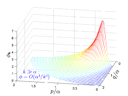
Figure 1: 3D plot of the ratio (19), which measures how much extra invariant $\tilde{I}$ is attached to a unit amount of energy with wave vector ${\bf k}$. This ratio is even in both “zonal” wavenumber $p=-\hat{\bm{\gamma}}\times{\bf k}$ and “radial” wavenumber $q=\hat{\bm{\gamma}}\cdot{\bf k}$, with the direction $\hat{\bm{\gamma}}$ defined in (3), and is plotted for $0.4<k/\alpha<2$. If one considers transporting a unit of energy from small scales (large $k$) toward the origin, one is forced to navigate around the peak, and squeeze into the valley along the $q$-axis.

To understand the significance of (18), and its relation to the formation of zonal flows, consider the linear combination $\tilde{I}=I-2\sqrt{3}\alpha E=\int\phi_{\bf k}E_{\bf k}d^{2}k/(2\pi)^{2}$, where $E_{\bf k}=\hat{X}^{E}_{\bf k}|\hat{\cal Q}_{\bf k}|^{2}$ is the energy spectrum, and

$$\phi_{\bf k} = \hat{X}^{M}_{\bf k}/\alpha\hat{X}^{E}_{\bf k}-2\sqrt{3}$$ (19)

$$= \left\{\begin{array}[]{ll}\frac{8\sqrt{3}\alpha^{4}p^{2}(q^{2}+p^{2}/5)}{k^{8}}+O[(\alpha/k)^{6}],&k/\alpha\gg 1\\ \frac{8\sqrt{3}\alpha^{4}p^{2}}{q^{2}(q^{2}+\alpha^{2})^{2}}+O[(p/q)^{4}],&p/q\ll 1.\end{array}\right.$$ (22)

Remarkably, $\hat{X}^{E}$ and $\hat{X}^{M}$ have identical (up to a factor $2\sqrt{3}\alpha$) asymptotic behavior for large $k$ and for small $p$, so $\hat{\phi}\to 0$ when $k\to\infty$ or $p\to 0$. The inverse cascade follows from the spectral balance needed to maintain conservation of energy and enstrophy foot:approx . As illustrated in Fig. 1 the extra conservation provides additional constraints leading to zonal flows. Specifically, it follows from (19) that a unit of energy at large $k/\alpha$ carries very small $\phi$. Therefore transferring energy towards the origin (either by local cascade, roughly along a level curve of $\phi$, or directly in a single jump) requires correspondingly small values of $p/q$: it must squeeze around the peak into the valley along the $q$-axis. The resulting flow is zonal with velocity along the $p$-axis, i.e., orthogonal to $\hat{\bm{\gamma}}$.

This conclusion is very general, following from a robust conservation law foot:tcons that operates under most situations considered in the literature. Bounds on spectral energy transport imposed by (18) should help inform future more detailed flow computations. Care, as well, should be taken in analyzing reduced models obtained from (1). The CHM equation CHM possesses the extra invariant, as well as enstrophy and the infinite potential vorticity hierarchy. However some generalizations of this equation fail to do so, at least in certain parameter ranges. Additional conservation might be restored by re-including some neglected terms.

References

- (1) P. H. Diamond, S.-I. Itoh, K. Itoh, and T. S. Hahm, Plasma Phys. Control. Fusion 47, R35 (2005).
- (2) P. H. Diamond, M. N. Rosenbluth, F. L. Hinton, M. Malkov, J. Fleischer, and A. Smolyakov, in 17th IAEA Fusion Energy Conference, Yokohama, Japan (International Atomic Energy Agency, Vienna, 1998) IAEA CN 69/TH3/1.
- (3) A. I. Smolyakov, P. H. Diamond, and V. I. Shevchenko, Phys. Plasmas 7, 1349 (2000).
- (4) T. D. Kaladze, D. J. Wu, O. A. Pokhotelov, R. Z. Sagdeev, L. Stenflo, and P. K. Shukla, Phys. Plasmas 12, 122311 (2005).
- (5) T. D. Kaladze, M. Shad, and L. V. Tsamalashvili, Phys. Plasmas 17, 022304 (2010).
- (6) C. P. Connaughton, B. T. Nadiga, S. V. Nazarenko, and B. E. Quinn, J. Fluid Mech. 654, 207 (2010)
- (7) V. E. Zakharov, in Breaking Waves IUTAM Symposium, Sydney, Australia, 1991, edited by M. L. Banner and R. H. J. Grimshaw (Springer, Berlin, 1992), pp. 69 -91.
- (8) J. G. Charney, Geophys. Publ. Oslo 17, 1 (1948); A. Hasegawa and K. Mima, Phys. Fluids 21, 87 (1978).
- (9) A. M. Balk, S. V. Nazarenko, and V. E. Zakharov, Phys. Lett. A 152, 276 (1991).
- (10) A. M. Balk, Phys. Lett. A 155, 20 (1991).
- (11) A. M. Balk and E. V. Ferapontov, in Nonlinear Waves and Weak Turbulence, edited by V. E. Zakharov (American Mathematical Society, Translations Series 2, Providence, RI, 1998), Vol. 182, pp. 1 -30.
- (12) A. M. Balk, F. van Heerden, and P. B. Weichman, Phys. Rev. E 83, 046320 (2011).
- (13) M. V. Nezlin and G. P. Chernikov, Plasma Phys. Reports 21, 922 (1995).
- (14) O. G. Onishchenko, O. A. Pokhotelov, R. Z. Sagdeev, P. K. Shukla, and L. Stenflo, Nonl. Processes Geophys. 11, 241 (2004).
- (15) Although much smaller in magnitude, the scalar nonlinearity is thought to be important because it greatly broadens the scale of wavenumbers that can lead to a modulational instability KWPSSS2005 .
- (16) Modern tokamaks (e.g., DIII-D, ITER) actually have non-circular poloidal cross-section, and the “radial” direction already involves noncircular geometry.
- (17) V. E. Zakharov and E. I. Schulman, Physica D 29, 283 (1988).
- (18) To be clear, once this condition is verified, it has indeed been proven that itself is conserved since the supplemental terms in (5) may be oscillatory, but are of higher order in amplitude.
- (19) The drift wave mode is not visible directly in (3), but may be projected out of the equations more directly using the refined field . This refinement basically serves to absorb the second term in (5) into . To linear order obeys the closed equation , hence obeys dispersion relation (13).
- (20) GHM also fails to conserve enstrophy.
- (21) Note that in the context of the CHM equation, drift wave enstrophy and energy are conserved exactly, while the extra invariant remains approximate. However, in the context of the hydrodynamic equations all three are approximate due to interaction with non-drift-wave modes.
- (22) By bounding the correction terms in , it follows that can accumulate relative errors at most over time : only for very large may conservation be violated. This assumes all corrections add in phase; more likely, phases are random, leading to even longer conservation. Also, conservation is enhanced for zonal flows, and hence will further improve as “condensation” toward large scales proceeds.