Swift observations of the 2006 outburst of the recurrent nova RS Ophiuchi:
III. X-ray spectral modelling

Abstract

Following the Swift X-ray observations of the 2006 outburst of the recurrent nova RS Ophiuchi, we developed hydrodynamical models of mass ejection from which the forward shock velocities were used to estimate the ejecta mass and velocity. In order to further constrain our model parameters, here we present synthetic X-ray spectra from our hydrodynamical calculations which we compare to the Swift data. An extensive set of simulations was carried out to find a model which best fits the spectra up to 100 days after outburst. We find a good fit at high energies but require additional absorption to match the low energy emission. We estimate the ejecta mass to be in the range $(2-5)\times 10^{-7}~{}{{\rm M}_{\odot}}$ and the ejection velocity to be greater than $6000{~{}{\rm km\,s}^{-1}}$ (and probably closer to $10,\!000{~{}{\rm km\,s}^{-1}}$). We also find that estimates of shock velocity derived from gas temperatures via standard model fits to the X-ray spectra are much lower than the true shock velocities.

1. Introduction

RS Ophiuchi (RS Oph) is one of the most well-studied of the ten known recurrent novae (RNe; Anupama 2008). The central system is a binary comprising a white dwarf (WD) and a red giant (RG) (Dobrzycka & Kenyon, 1994). A classical nova outburst involves mass transfer from the companion to the WD. The build-up of pressure and temperature in the degenerate layer of accreted hydrogen eventually leads to a thermonuclear runaway (TNR) on the surface of the WD, resulting in the high-speed ejection of a shell of material into the circumstellar medium (Starrfield, 2008). Novae which have been observed in outburst more than once are called RNe. The shock interaction of the ejecta with the surrounding medium has been found to heat the gas to temperatures of $10^{7}-10^{8}$ K, yielding hard X-ray radiation (Lloyd et al. 1992; O’Brien, Lloyd & Bode 1994; Mukai & Ishida 2001). In the case of RS Oph, the ejecta run into the surrounding dense RG wind. Soft X-ray emission is also expected to be revealed later in the outburst from a central WD close to Eddington luminosity (Krautter et al. 1996; Balman, Krautter & Oegelman 1998) as is seen in RS Oph (see below).

RS Oph has had outbursts recorded in 1898, 1933, 1958, 1967, 1985 (see Rosino 1987; Rosino & Iijima 1987) and most recently on 2006 February 12 (Narumi et al., 2006), with possible additional outbursts in 1907 and 1945 (Schaefer 2004; Oppenheimer & Mattei 1993). Its binary system has an orbital period of $455.72\pm 0.83$ days (Fekel et al., 2000). The mass of the WD is suspected to be close to the Chandrasekhar limit from various considerations, including the speed class of outburst and the relatively short recurrence time between outbursts (e.g. Yaron et al. 2005, Sokoloski et al. 2006, Hachisu et al. 2007). The distance to RS Oph is 1.6 kpc (Bode 1987; see also Barry et al. 2008).

RS Oph was detected in X-rays just 2 days after the 2006 outburst with the RXTE satellite (Sokoloski et al., 2006) and 3.17 days after outburst using the XRT instrument on board the Swift satellite (Bode et al. 2006, hereafter Paper I). The Swift observations were performed on average every one or two days during the first 100 days, covering all the phases of the remnant’s evolution. The rate of observations subsequently decreased but continued for more than a year (Page et al., 2008). RS Oph was seen initially as a source of fairly hard X-rays, gradually softening with time. Around 26 days after outburst, the very bright and soft component from the Super-Soft Source (SSS) phase of nuclear burning on the surface of the WD appeared in the spectrum (Osborne et al. 2006; Hachisu et al. 2007; Page et al. 2008; Osborne et al. 2011).

In an effort to improve on the models of the 1985 outburst and, in particular, to address the new observations of the early phases of its evolution, we developed new hydrodynamical models for RS Oph (Vaytet, O’Brien & Bode 2007, hereafter Paper II). We used a one-dimensional Eulerian second order Godunov code (O’Brien et al., 1994) to simulate the outburst where mass-loss in the form of a fast wind from the WD ran into a surrounding slow RG wind. The scheme took into account all three phases of the remnant’s evolution, and allowed us, after a thorough analysis of the shock velocities, to determine that the ejecta had a low mass ($\sim 2\times 10^{-7}~{}{{\rm M}_{\odot}}$) and a high ejection velocity. The models also showed that radiative cooling had an important impact on the evolution of the shocks; the amount of energy radiated by the hot ejecta was correlated to the rate at which the forward shock velocity decreased in time.

In Paper II our analysis relied on single-temperature fits to the Swift X-ray spectra (from Paper I) in order to determine post-shock temperatures and hence the shock velocities. Here we improve on this approach by calculating full X-ray spectra directly from our hydrodynamical results using xspec and by including the effects of overlying absorption and instrument response. Results from an extensive set of simulations are compared to the Swift observations for the first 100 days after outburst in order to obtain best-fitting values for the model parameters.

2. Swift XRT observations

Some 70 observational epochs of RS Ophiuchi were obtained using the X-ray Telescope (XRT) onboard the Swift observatory during the first 100 days after the 2006 outburst. As in Paper I, the data were processed using the standard Swift software and source spectra were extracted from the cleaned Windowed Timing (WT) mode ($t<90$ days) and Photon Counting (PC) mode ($t>90$ days) event lists. Because of the high count rate of the X-ray source, most of the WT were piled-up. Thus, the core of the PSF was excluded: an outer box of width $60\times 20$ pixels was used, with the central 10 pixels (1 pixel = $2\arcsec 36$) removed. Similarly, the PC data were piled-up: here, an annulus with outer radius 30 pixels was used, with the inner exclusion radius decreasing from six to zero pixels between days 90 and 100. Background spectra were obtained from nearby source-free regions, using a $60\times 20$ pixel box for the WT data and a 60 pixel radius circle for the PC. We corrected for the fractional loss of the point-spread function caused both by the exclusion of the central (piled-up) region and the positioning of the source over the bad CCD columns (caused by micrometeorite damage on 2005 May 2007; Abbey et al. 2006) when calculating the count rate and flux.

Grades 0–2 and 0–12 were chosen for the spectral analysis of the WT and PC data respectively. The FTOOL xrtmkarf was used to generate suitable ancillary response function files, and these were used in conjunction with the relevant response matrices. All spectra were grouped to a minimum of 20 counts per bin in order to facilitate the use of $\chi^{2}$ statistics in xspec, the results of which are shown in Fig. 1 (black crosses) for 8 epochs.

3. Calculation of synthetic X-ray spectra

Our hydrodynamical models from Paper II predict the physical conditions of the hot shocked gas at any time during the outburst. In practise the model comprises many concentric spherical shells each with a different temperature and density. Since it would be too computationally intensive to calculate the X-ray emission from each shell separately, we grouped them into 30 logarithmically-divided temperature bins from $10^{4}$ to $10^{9}$ K, weighting each shell’s contribution by its emission measure (experiment suggested 30 bins were sufficient to give an accurate result). These were then fed as a 30-component plasma into xspec (version 12), an X-ray data reduction and spectrum calculation code. This was used to compute the X-ray spectrum with the MEKAL model for emission from hot, diffuse gas, including line emissions from C, N, O, Ne, Na, Mg, Al, Si, S, Ar, Ca, Fe and Ni, along with free-free, free-bound and two-photon emission (for more details see Vaytet 2009; Mewe et al. 1986).

The interstellar equivalent hydrogen absorption column for our models was taken from Hjellming et al. (1986) who found $n_{H}=(2.4\pm 0.6)\times 10^{21}~{}\mathrm{cm}^{-2}$. We have also included a contribution from the circumstellar absorption due to the RG wind surrounding the hot, shocked gas behind the forward shock. At each epoch we calculate an average value for this circumstellar absorption across the face of the sphere of shocked gas.

Of course, only the unshocked neutral part of the RG wind will contribute to absorption. It is however non-trivial to know the ionisation state of the RG wind at all times, since a large portion of it could be ionised by the radiation emitted during the outburst. This requires not only knowledge of the recombination rates in the RG wind but also knowledge of the luminosity of the central radiation source at all times, which is clearly not constant nor simple to model (see for example Page et al. 2008). O’Brien, Bode & Kahn (1992) assumed that the whole RG wind was flash-ionised by UV radiation at the very beginning of the outburst, then computed recombination rates inside the RG wind. Here we simply use upper and lower extremes; either the RG wind is fully neutral or fully ionised. We are then confident that the correct absorption has to lie between these limits since they do not depend on any assumptions about the central radiation field.

The final step in the creation of the synthetic spectra was to fold the results through the Swift XRT instrumental response matrix. The response used here was the same as for the observations mentioned above, with the corresponding ancillary file specific to each observation to provide the precise effective area of the detector and correct for bad channels. We used the canonical distance of 1.6 kpc for normalisation.

4. Results

4.1. Initial simulations from Paper II

Model runs 1 to 16 presented in this section are identical to those in Paper II; see Table LABEL:tab:params for a list of parameter values. Run 14 is not included since it represented a continuous fast wind ejection during the entire duration of the simulation, thus rendering parameters such as ejected mass $M_{\mathrm{ej}}$ and outburst energy $E_{0}$ meaningless.

Fig. 1 shows the synthetic spectra for five of these simulations compared with the Swift observations. Results are shown in separate panels for days 3, 5, 11, 18, 29, 50, 75 and 100 after outburst. Each panel includes results assuming the overlying RG wind is either fully neutral (solid line) or fully ionised (dashed line). We first consider the results from run 2 (shown in black), a fairly typical example. At early times ($3-18$ days), before the SSS component from the WD remnant appears at the soft end of the spectrum, the synthetic spectra clearly do not match the observations; the model is overestimating the soft X-ray count rates and underestimating the hard count rates. We do not include the SSS component in our models so for later times (day 29 and after), the Swift data at the soft end of the spectrum has been omitted (energies $\lesssim 1$ keV). At these late times, at the hard end of the spectrum the model count rates are very closely matched to the observations, suggesting that the hard count rates have decreased faster in the observations than in the model.

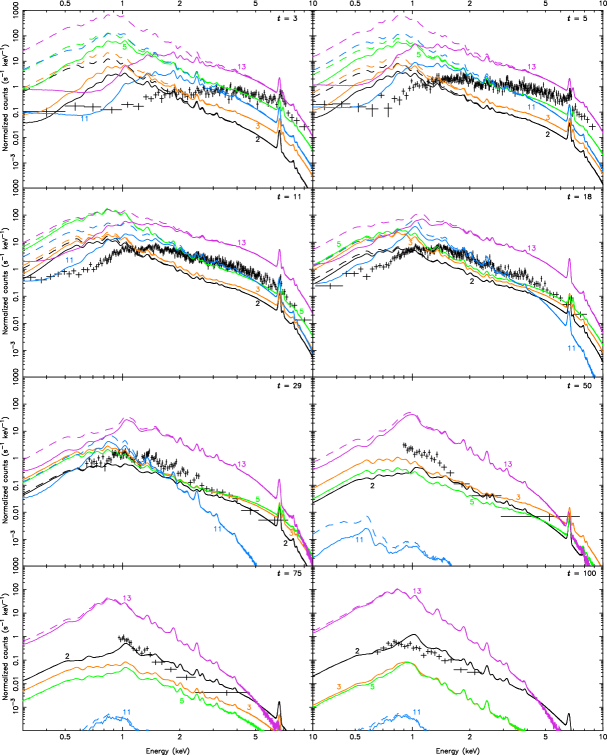
Figure 1.— Synthetic X-ray spectra for runs 2 (black), 3 (orange), 5 (green), 11 (blue) and 13 (dark pink) at days 3, 5, 11, 18, 29, 50, 75 and 100. The solid and dashed lines represent a fully neutral and fully ionised RG wind, respectively. The black crosses represent the Swift data. The Swift data at low energies for days 29 and after showing the SSS component have been removed since no SSS is included in our models.

In order to link the synthetic spectra with the hydrodynamics, we recall Fig. 5 in Paper II where we concluded that the deceleration rate of the forward shock was an important aspect of the shock models. We concluded that runs 3 and 11 have forward shock deceleration rates lower and higher than run 2, respectively. Their X-ray spectra are shown in Fig. 1 (orange for run 3 and blue for run 11).

In run 3 (orange), the increased $M_{\mathrm{ej}}$ increases the X-ray count rates, this effect being strongest at the hard end of the spectrum. The hard X-ray count rates decrease more slowly than in run 2, which is due to the higher inertia that the shell carries due to its higher mass. This is best seen at days 18 to 50. Days 75 and 100 should be ignored in this case as by this time the shock has reached the edge of the RG wind; see Fig. 4 in Paper II.

In the case of run 11 (blue), the high fast wind velocity $V_{2}$ also increases the X-ray count rates, but this time over the whole energy spectrum, most probably simply due to the higher outburst energy compared to run 2. In run 11 both hard and soft X-ray count rates decrease much faster than in runs 2 and 3, falling to the bottom of the visible plot area by day 75. Note that for run 11 the shock does not reach the edge of the wind on a 100-day timescale. Finally, the impact of absorption in the overlying high-density neutral RG wind in run 11 (solid blue line) is clearly visible on the soft part of the spectrum at early times where the predicted count rates are more consistent with observations.

Further, by simply increasing $V_{2}$ and leaving $M_{\mathrm{ej}}$ untouched as in run 5 (Fig. 1; green lines), we note that the count rates are also greatly increased across the spectrum. Runs 3 and 5 have identical outburst energies and RG wind densities; it is hence not surprising to see that their X-ray spectra are very similar at late times (day 29 and after) apart from the hard count rates being slightly higher in run 3 at day 50. Comparing run 5 with run 11 reveals that increasing $V_{2}$ can only be effective in enhancing hard count rates at early times if $M_{\mathrm{ej}}$ is not too low.

We conclude that, as one might expect, greater deceleration of the forward shock results in faster reduction in hard X-ray count rates. This is also sensitive to the ejected mass $M_{\mathrm{ej}}$; a high-mass shell will carry more momentum and therefore decelerate more slowly. A high ejection velocity $(V_{2}\geq 5000{~{}{\rm km\,s}^{-1}})$ greatly overestimates the soft count rates. Note that the strong Fe XXV K line at 6.7 keV appears wider in the Swift observations than in our models (run 2 for example). We do not include Doppler broadening in our models but it should also be noted that a second Fe XXVI line (6.97 keV) appears very close to the first in some of our models (runs 3, 5 and 13) which would not be resolved by the XRT and would broaden the appearance of the Fe line. Finally, it is clear from runs 2 and 3 that a relatively low-density (even entirely neutral) RG wind appears not to produce sufficient absorption of low-energy X-rays at early times.

In Paper II, run 13 provided the best fit to the forward shock velocities. However the extremely high implied $V_{2}$ of 16,300 km s^-1, for which there was little evidence elsewhere, cast some doubt on the validity of the model. The synthetic spectra for run 13 are shown in Fig. 1 (dark pink). These clearly show run 13 does not match the observations of the 2006 outburst of RS Oph. Although the desired large amount of absorption is present at early times, the count rates are overestimated across the spectrum at every epoch.

4.2. Fitting synthetic spectra to the Swift data

A fuller exploration of the parameter space of the hydrodynamical model has now been undertaken by carrying out a new extensive set of simulations using the same code as in Paper II. This brings the total number of runs to 88. All the parameters for runs 1 to 88 are listed in Table LABEL:tab:params (run 14 excluded for reasons given above).

Table 1ASPHERE code parameter space

Run	RG wind	Fast wind	Fast wind	Outburst	Ejected	RG wind	Mass ratio	RG wind	Fast wind	Mean flux difference
	mass-loss	mass-loss	velocity	energy	mass	mass	$M_{\mathrm{ej}}/M_{\mathrm{RGW}}$	ratio	phase	total	early	late
	$\dot{M_{1}}$	$\dot{M_{2}}$	$V_{2}$	$E_{0}$	$M_{\mathrm{ej}}$	$M_{\mathrm{RGW}}$	$R$	$\dot{M_{1}}/u$	$t_{0}$	$\Phi_{T}$	$\Phi_{E}$	$\Phi_{L}$
	($\!\times 10^{-7}$ ${\rm M}_{\odot}$/yr)	($\!\times 10^{-7}$ ${\rm M}_{\odot}$/yr)	($\!{~{}{\rm km\,s}^{-1}}$)	($\!\times 10^{43}$ erg)	($\!\times 10^{-6}~{}{{\rm M}_{\odot}}$)	($\!\times 10^{-6}~{}{{\rm M}_{\odot}}$)		($\!\times 10^{12}$ g/cm)	(days)		($t<30$d)	($t\geq 30$d)
1	1.43	158.59	3000	1.85	0.24	3.00	0.080	6.00	7.0	0.961	0.940	0.965
2	1.43	730.62	3000	8.62	1.10	3.00	0.367	6.00	7.0	0.574	0.748	0.537
3	1.43	3171.80	3000	36.94	4.78	3.00	1.595	6.00	7.0	0.484	0.570	0.465
4	1.43	730.62	1398	1.85	1.10	3.00	0.367	6.00	7.0	0.997	0.995	0.998
5	1.43	730.62	6251	36.94	1.10	3.00	0.367	6.00	7.0	0.611	0.311	0.676
6	1.43	730.62	3500	11.58	1.10	3.00	0.367	6.00	7.0	0.442	0.661	0.395
7	1.43	730.62	4000	15.13	1.10	3.00	0.367	6.00	7.0	0.411	0.567	0.378
8	1.43	5113.73	3000	8.62	1.10	3.00	0.367	6.00	1.0	0.528	0.628	0.506
9	1.43	340.97	3000	8.62	1.10	3.00	0.367	6.00	15.0	0.660	0.746	0.642
10	6.34	730.62	3000	8.62	1.10	13.32	0.083	26.67	7.0	0.995	0.974	1.000
11	6.34	79.30	12000	14.77	0.12	13.32	0.009	26.67	7.0	0.853	0.259	0.980
12	1.43	1148.03	3969	8.62	1.10	3.00	0.367	6.00	7.0	0.567	0.697	0.539
13	9.52	158.59	16300	46.73	0.20	19.98	0.010	40.00	6.0	17.956	6.491	20.413
15	1.43	298.62	3000	3.48	0.45	3.00	0.150	6.00	7.0	0.634	0.849	0.588
16	1.43	497.66	3000	5.80	0.75	3.00	0.250	6.00	7.0	0.620	0.786	0.584
17	7.93	158.59	9000	9.50	0.14	16.65	0.008	33.33	4.0	0.986	0.921	1.000
18	52.33	852.29	4500	19.14	1.10	110.00	0.010	220.20	6.0	4.160	0.728	4.895
19	7.93	774.82	8000	55.00	1.00	16.65	0.060	33.33	6.0	19.847	6.348	22.740
20	6.34	126.87	10000	16.42	0.19	13.32	0.014	26.67	7.0	0.748	0.375	0.828
21	6.34	174.45	7000	11.06	0.26	13.32	0.020	26.67	7.0	0.975	0.863	1.000
22	7.93	451.57	7000	24.54	0.58	16.65	0.035	33.33	6.0	1.099	1.276	1.061
23	7.93	323.49	8000	22.96	0.42	16.65	0.025	33.33	6.0	0.908	0.877	0.915
24	7.93	646.97	7000	35.16	0.83	16.65	0.050	33.33	6.0	10.241	3.533	11.678
25	7.93	646.97	6000	25.83	0.83	16.65	0.050	33.33	6.0	1.223	1.534	1.157
26	7.93	646.97	5000	17.94	0.83	16.65	0.050	33.33	6.0	0.939	0.655	0.999
27	7.93	774.82	4500	17.40	1.00	16.65	0.060	33.33	6.0	0.958	0.763	0.999
28	7.93	1035.15	4500	23.25	1.34	16.65	0.080	33.33	6.0	0.775	0.408	0.853
29	7.93	1293.95	4500	29.06	1.67	16.65	0.100	33.33	6.0	2.973	1.578	3.272
30	7.93	1164.56	4000	20.67	1.50	16.65	0.090	33.33	6.0	0.901	0.466	0.995
31	7.93	1578.30	4500	35.45	2.04	16.65	0.122	33.33	6.0	8.992	2.471	10.390
32	7.93	1940.92	4500	43.59	2.51	16.65	0.150	33.33	6.0	14.352	3.447	16.688
33	7.93	2587.89	4500	58.12	3.34	16.65	0.201	33.33	6.0	17.011	4.900	19.606
34	7.93	1578.30	4000	28.01	2.04	16.65	0.122	33.33	6.0	2.124	1.351	2.289
35	7.93	1940.92	4000	34.44	2.51	16.65	0.150	33.33	6.0	8.035	2.174	9.291
36	7.93	2587.89	4000	45.92	3.34	16.65	0.201	33.33	6.0	14.954	3.296	17.452
37	7.93	1578.30	3500	21.44	2.04	16.65	0.122	33.33	6.0	0.862	0.368	0.968
38	7.93	1940.92	3500	26.37	2.51	16.65	0.150	33.33	6.0	0.986	0.915	1.001
39	7.93	2587.89	3500	35.16	3.34	16.65	0.201	33.33	6.0	7.962	2.065	9.225
40	7.93	155.28	12000	24.80	0.20	16.65	0.012	33.33	6.0	1.366	1.745	1.284
41	7.93	182.39	12000	29.13	0.24	16.65	0.014	33.33	6.0	4.023	2.979	4.247
42	7.93	232.91	12000	37.20	0.30	16.65	0.018	33.33	6.0	13.453	4.468	15.378
43	7.93	284.67	12000	45.46	0.37	16.65	0.022	33.33	6.0	19.062	5.674	21.931
44	7.93	155.28	10500	18.99	0.20	16.65	0.012	33.33	6.0	0.885	0.349	0.999
45	7.93	182.39	10500	22.30	0.24	16.65	0.014	33.33	6.0	0.845	0.750	0.866
46	7.93	232.91	10500	28.48	0.30	16.65	0.018	33.33	6.0	3.182	2.736	3.277
47	7.93	284.67	10500	34.81	0.37	16.65	0.022	33.33	6.0	10.973	3.949	12.478
48	7.93	155.28	9300	14.89	0.20	16.65	0.012	33.33	6.0	0.969	0.827	1.000
49	7.93	182.39	9300	17.50	0.24	16.65	0.014	33.33	6.0	0.938	0.649	0.999
50	7.93	232.91	9300	22.34	0.30	16.65	0.018	33.33	6.0	0.841	0.730	0.865
51	7.93	284.67	9300	27.31	0.37	16.65	0.022	33.33	6.0	2.154	2.374	2.107
52	7.93	905.76	7000	49.22	1.17	16.65	0.070	33.33	6.0	19.007	5.449	21.912
53	7.93	1100.23	7000	59.79	1.42	16.65	0.085	33.33	6.0	19.088	6.562	21.773
54	7.93	1397.76	7000	75.96	1.80	16.65	0.108	33.33	6.0	16.828	7.970	18.727
55	7.93	905.76	6300	39.87	1.17	16.65	0.070	33.33	6.0	13.575	4.101	15.606
56	7.93	1100.23	6300	48.43	1.42	16.65	0.085	33.33	6.0	18.193	5.128	20.993
57	7.93	1397.76	6300	61.53	1.80	16.65	0.108	33.33	6.0	18.542	6.502	21.122
58	7.93	905.76	5500	30.39	1.17	16.65	0.070	33.33	6.0	4.534	2.305	5.011
59	7.93	1100.23	5500	36.91	1.42	16.65	0.085	33.33	6.0	10.771	3.322	12.368
60	7.93	1397.76	5500	46.89	1.80	16.65	0.108	33.33	6.0	16.799	4.490	19.437
61	1.90	1278.39	4000	15.12	1.10	4.00	0.275	8.00	4.0	0.446	0.381	0.460
62	1.90	1110.13	4000	13.13	0.96	4.00	0.239	8.00	4.0	0.549	0.406	0.579
63	1.90	951.54	4000	11.26	0.82	4.00	0.205	8.00	4.0	0.649	0.426	0.697
64	1.90	792.95	4000	9.38	0.68	4.00	0.171	8.00	4.0	0.761	0.473	0.823
65	1.90	634.36	4000	7.50	0.55	4.00	0.137	8.00	4.0	0.713	0.529	0.753
66	1.90	475.77	4000	5.63	0.41	4.00	0.102	8.00	4.0	0.553	0.604	0.542
67	1.90	622.94	4000	5.53	0.40	4.00	0.101	8.00	3.0	0.561	0.585	0.555
68	1.90	817.64	4000	4.84	0.35	4.00	0.088	8.00	2.0	0.508	0.582	0.492
69	1.90	560.68	4000	4.15	0.30	4.00	0.075	8.00	2.5	0.481	0.638	0.448
70	1.90	507.49	4500	5.70	0.33	4.00	0.082	8.00	3.0	0.567	0.542	0.573
71	1.90	364.76	4500	5.46	0.32	4.00	0.079	8.00	4.0	0.522	0.577	0.511
72	1.90	293.39	5000	6.78	0.32	4.00	0.079	8.00	5.0	0.635	0.505	0.663
73	1.90	285.46	5500	7.98	0.31	4.00	0.077	8.00	5.0	0.744	0.427	0.812
74	1.90	285.46	6000	9.50	0.31	4.00	0.077	8.00	5.0	0.760	0.389	0.840
75	1.90	269.60	6500	10.53	0.29	4.00	0.073	8.00	5.0	0.702	0.448	0.757
76	1.43	198.24	8000	11.73	0.21	3.00	0.071	6.00	5.0	0.366	0.340	0.372
77	4.76	713.66	5000	16.49	0.77	10.00	0.077	20.00	5.0	3.179	0.732	3.703
78	1.90	182.38	8000	15.10	0.28	4.00	0.069	8.00	7.0	0.378	0.300	0.394
79	7.93	1744.49	4500	45.71	1.13	16.65	0.068	33.33	3.0	0.859	0.274	0.984
80	7.93	2061.67	5000	28.58	1.33	16.65	0.080	33.33	3.0	5.522	2.841	6.097
81	1.90	158.59	10000	23.45	0.27	4.00	0.068	8.00	8.0	0.462	0.657	0.420
82	1.90	111.01	10000	20.52	0.24	4.00	0.060	8.00	10.0	0.462	0.637	0.424
83	1.90	364.76	10000	20.23	0.24	4.00	0.059	8.00	3.0	0.461	0.762	0.397
84	1.90	491.63	6000	9.81	0.32	4.00	0.079	8.00	3.0	0.749	0.474	0.807
85	1.90	388.55	8000	10.16	0.32	4.00	0.080	8.00	6.0	0.747	0.367	0.828
86	1.90	888.10	6000	11.82	0.38	4.00	0.096	8.00	2.0	0.590	0.442	0.621
87	7.93	951.54	5000	26.38	1.23	16.65	0.074	33.33	6.0	1.132	1.289	1.098
88	1.43	730.62	8000	60.45	1.10	3.00	0.367	6.00	7.0	0.514	0.660	0.495
Notes.–The slow wind velocity is $u=15{~{}{\rm km\,s}^{-1}}$ throughout (Paper II). Run 14 is omitted (see section 4.1 and Paper II).

In Paper II, we concluded that the deceleration rate of the forward shock was directly related to the amount of energy radiated away by the ejecta. This in turn appeared to be related to the ratio of the ejected mass to the mass contained in the RG wind; the lower the ratio, the higher the fraction of energy which was radiated away. In Table. LABEL:tab:params we also list this ratio $R=M_{\mathrm{ej}}/M_{\mathrm{RGW}}$ for each run.

In order to assess the goodness of fit of each run’s synthetic spectra to the Swift data, we extracted fluxes from our models in order to compare them directly to the fluxes observed in some 70 Swift observations between day 3 and day 100. In all cases, the fluxes have been taken in the energy range $1-10$ keV in order to avoid contamination from the SSS emission. The absolute value of the difference between the model and observed fluxes as a fraction of the observed flux was calculated for each epoch. These were then summed over all epochs and an average was taken, giving the total mean fractional flux difference $\Phi_{T}$. We also define two other quantites $\Phi_{E}$ and $\Phi_{L}$ which are the early ($t<30$ days) and late ($30<t<100$ days) mean fractional flux differences respectively. These values are listed for all runs in Table LABEL:tab:params. All the values quoted are for runs with a fully-neutral RG wind. It is evident from the Swift observations that some absorption is present in the spectra, and listing the mean flux differences for the synthetic spectra with an ionised RG wind is therefore unecessary. Moreover, the effect of circumstellar absorption is highest at the soft end of the energy spectrum (see Fig. 1) and since we only consider energies in the range $1-10$ keV, total mean flux differences for ionised and neutral RG winds are in almost all cases very similar.

The total mean flux differences are a useful way of identifying the regions in the parameter space which yield best fitting runs, however it is not an absolute measure of the quality of the fits. For instance run 11 would be classed as one of the best fitting runs according to $\Phi_{E}$ (Table LABEL:tab:params), but the model spectra at days 3 and 5 (see Fig. 1) are clearly not good fits to the data as the spectral slope is very different to the observations. The over-estimate in medium energy counts ($1.0-2.5$ keV) compensates for the underestimate at the hard energy end, giving a total flux very close to the observed flux. We exclude any runs with large $\Phi$ values. We also examined all the spectra by eye to ensure that we had not excluded runs which had the correct spectral shape but were lying either above or below the Swift data at all epochs. Indeed, such a systematic error could be corrected simply by varying the distance to RS Oph, which has been subject to some debate (Barry et al., 2008). After this exhaustive analysis, we have come to the following conclusions (ejecta masses are given in $10^{-6}~{}{{\rm M}_{\odot}}$):

• For all runs, in order to reproduce the correct amount of hard X-ray emission, we require $V_{2}\geq 6000{~{}{\rm km\,s}^{-1}}$

• If $M_{\mathrm{ej}}>1.5~{}(\times 10^{-6}~{}{{\rm M}_{\odot}})$, spectra can be a good match at early times ($t<5$ days) but are much too bright at later times (e.g. run 33)

• If $0.8<M_{\mathrm{ej}}\leq 1.5$:

  - if $\dot{M_{1}}$ is high, the X-ray flux is either too high (run 19) or fades too quickly (run 25)

  - if $\dot{M_{1}}$ is low, a high $V_{2}\geq 6000{~{}{\rm km\,s}^{-1}}$ forces the fluxes to be too high and the deceleration rate of the forward shock to be too low (run 88)

• If $0.2<M_{\mathrm{ej}}\leq 0.8$:

  - if $\dot{M_{1}}$ is high, the X-ray flux is either too low for very low masses (run 48) or fades too quickly (runs 23, 45)

  - if $\dot{M_{1}}$ is low, hard X-ray counts are too low for $V_{2}<8000{~{}{\rm km\,s}^{-1}}$ (run 73)

  - a good fit is found for the hard X-rays at all epochs if $\dot{M_{1}}$ is low and $V_{2}\geq 8000{~{}{\rm km\,s}^{-1}}$

• If $M_{\mathrm{ej}}<0.2$, the hard X-ray flux is too low and the fluxes at all energies fade very rapidly (runs 11, 17)

This step by step elimination process leads us to believe that the mass ejected in the outburst $M_{\mathrm{ej}}$ is in the range $(2-8)\times 10^{-7}~{}{{\rm M}_{\odot}}$. We find our best fitting model to be run 81 (see Fig. 2), although even this does show a small overestimate in hard X-rays around day 29. Its main characteristics are its low $M_{\mathrm{ej}}=2.7\times 10^{-7}~{}{{\rm M}_{\odot}}$ and high $V_{2}=10^{4}{~{}{\rm km\,s}^{-1}}$.

Figure 2.— Synthetic X-ray spectra for run 81 at days 3, 5, 11, 18, 29, 50, 75 and 100. The thin solid and dashed lines represent a fully neutral and fully ionised RG wind, respectively. The bold solid line represents the spectrum including additional absorption. The additional hydrogen equivalent absorption columns are (in units of $10^{-21}~{}\mathrm{cm}^{-2}$): 4.0 (day 3), 2.5 (day 5), 0.5 (day 11) and 0.3 (day 18). The black crosses represent the Swift data. The dot-dash line in the top left panel represents the contribution to the total X-ray spectra from the post-forward shock material (see end of section 4.3).

The majority of the runs produce too many low energy X-rays. We have investigated whether this might be due to insufficient circumstellar absorption. In order to naturally increase the absorption, we simply increased the slow wind mass-loss rate (see for example the difference in the amount of absorption in runs 2 and 11) but of course this has a significant effect on the shock dynamics. With a denser RG wind, if we wish to produce shock velocities high enough to be consistent with observations, we have to vastly increase $V_{2}$. This leads to an overestimate of the soft and medium energy count rates  (see run 13 for example). In order to obtain flat spectra at early times (days 3 and 5, say), we have had to keep $V_{2}$ in the range $\sim 5000-10000{~{}{\rm km\,s}^{-1}}$ and consequently the mass-loss rate into the RG wind $\dot{M}_{1}$ also needs to be relatively low. A mid-range $M_{\mathrm{ej}}$ was then required to obtain the correct hard X-ray decay rate, as in run 81.

An alternative way of addressing the deficit in absorption of soft X-rays is to include some additional ad-hoc absorption during the calculation of the spectrum (shown as bold solid lines in Fig. 2). This allows us to produce good agreement between the synthetic spectra and the Swift observations. The resulting total absorption column (including the ISM, the CSM from the RG wind and the ad-hoc additional absorption) is within the same order of magnitude as the absorption column required by the fits to the Swift data in Paper I. Such additional absorption could be due to the presence of a dense gas torus close to the binary core, as suggested by the IR observations of Evans et al. (2007).

Of course, we have to acknowledge that such a dense torus would have an effect on the dynamics of the shocks propagating through the CSM but this is a problem that can only be addressed in 2D or 3D simulations. Furthermore, such a dense torus will play a role in the bipolarity seen in the radio (O’Brien et al., 2006; Sokoloski et al., 2008; Rupen et al., 2008) and optical imaging (Bode et al., 2007; Ribeiro et al., 2009). Indeed, Walder et al. (2008) have shown in full 3D hydrodynamical simulations that the orbiting accreting WD leaves a spiral wake in the RG wind along with a slight equatorial density enhancement, and that the high-density accretion disk around the WD has a substantial size ($3\times 10^{12}$ cm in diameter). They illustrate the ejecta collimation efficiency of these features during the nova outburst. Orlando et al. (2009) have also computed the X-ray emission from 3D simulations of the outburst in a wind with an equatorial density enhancement but unfortunately do not show the absorption effect of the presence of such an enhancement on the resulting synthetic spectra.

4.3. Shock position, velocities and flux comparisons

Figure 3 shows the run 81 forward shock position in milli-arcseconds (mas) assuming a distance of 1.6 kpc as a function of time (black solid line), compared to the size measurements of three separate features in resolved radio-interferometry images. The radio images of O’Brien et al. (2008), Rupen et al. (2008) and Sokoloski et al. (2008) have indeed revealed three main synchrotron emitting features (most probably associated with shocks) in the remnant of RS Oph: a central expanding ring, an eastern lobe further away from the central binary system and an additional western counterpart. The positions of the lobes and the size of the expanding ring measured in the radio observations are represented by the various points (see legend for details).

Figure 3.— Run 81 forward shock position as a function of time (solid line) compared to the radio imaging measurements of the size of the expanding ring and the position of the eastern and western lobes by O’Brien et al. (2008), Rupen et al. (2008) and Sokoloski et al. (2008). The error bars have been omitted for clarity; on the VLBI and VLBA measurements they are $\sim 1$ mas, on the MERLIN data they are $\sim 10$ mas.

It seems natural to compare the position of our spherically symmetric shock to the size of the expanding ring. We first note that the position of the run 81 forward shock is higher than the early ring size measurements ($t<30$ days) by a factor of about two. At later times ($30<t<50$ days), it is very consistent with the ring size measurements of Sokoloski et al. (2008), before it breaks out of the RG wind (kink circa day 44). Between days 20 and 45, the model shock position is also close to the position of the western lobe measured by O’Brien et al. (2008). It is however never close to the measured positions of the eastern lobe until the shock breakout. We conclude that our model shock positions are consistent with a distance of 1.6 kpc and that over-estimates at early times arise from the fact that we are trying to reproduce the X-ray emission of a system with multiple ejection features moving at different speeds with a spherically symmetric model. The model shock positions sensibly lie between the ring sizes and the eastern lobe positions, as a compromise between the two.

Figure 4a shows the forward shock velocities (solid line) measured directly from the hydrodynamical simulation of run 81. These are compared to the shock velocities estimated in Paper I from single-temperature fits to the Swift spectra (empty squares with error bars) and to the IR velocities from Das, Banerjee & Ashok (2006) (triangles). The IR velocities were taken from the full width zero intensity (FWZI) of the Oi and Pa$\beta$ emission lines. The velocities from the RXTE X-ray data of Sokoloski et al. (2006) are also shown (crosses).

Figure 4b shows the total $1-10$ keV X-ray fluxes from the Swift observations (empty squares) compared to the fluxes calculated from run 81 (solid line; including the additional ad-hoc absorption). The model fluxes are consistent with the observed fluxes. The early turnover after an initial rise around day 6 occurs at the same time in both model and observations. There is also a clear break in the model curve just after day 40 which appears to fit the data; this corresponds to the time when the model forward shock breaks out of the RG wind. This occurs at the same time as the dramatic increase in the model velocities.

Figure 4.— Run 81 results compared to Swift data from Paper I and IR data from Das et al. (2006). (a) Forward shock velocities: the black empty squares represent the Swift data, the red triangles the IR data (filled = Oi; empty = Pa$\beta$) and the solid line the model. The IR velocities were taken from the FWZI/2 of the emission lines. The dashed line is the velocities derived from the $T$ fits to our synthetic spectra. The dotted line represents the gas velocity behind the reverse shock. The crosses are the Sokoloski et al. (2006) RXTE data. (b) X-ray flux (in the range $1-10$ keV): the empty squares represent the Swift observations and the solid line the model. Error bars here are smaller than the size of the squares ($<5\%$).

While the X-ray fluxes are well reproduced, the model velocities do not agree with the Paper I velocities derived from the X-ray observations. The model velocities are much higher, the early turn-over occurs about $4-5$ days later and the deceleration rate is slower. There is however reasonable agreement between the velocities obtained in Paper I and those by Sokoloski et al. (2006) from RXTE observations. It has been pointed out by Tatischeff & Hernanz (2008) and references therein that equation (3) in Paper I for strong shock dynamics can underestimate shock velocities where non-linear diffusive shock acceleration of particles is efficient, which is most probably the case for RS Oph. We also note that the immediately post-shock gas is the hottest and would provide the best estimate of the shock velocity. However, the observed spectrum is made up from contributions from a wide range of gas temperatures, emission from the shocked ejecta and even perhaps the WD remnant. These will lead to a softening of the spectrum and so velocities computed from single-temperature fits will be biased towards lower temperatures and hence lower derived shock velocities.

The IR velocities shown in Fig. 4a are in better agreement with the model forward shock velocities. However it should be emphasised that the different methods are likely to be biased towards emission from different parts of the expanding remnant. This spans a wide range of velocities, including the unshocked and shocked fast wind from the WD, and the shocked (and unshocked) RG wind. We also show in Fig. 4a the gas velocity just after the reverse shock (blue solid line), which is in very good agreement with the IR velocities at early times. Taking the FWZI of the IR lines probes only the fastest moving material in the system, which suggests that the IR line widths are first dominated by the post reverse shock gas and only later by the post forward shock gas.

As previously discussed, in this spherically symmetric model the shock wave breaks out of the RG wind just after day 40, leading to a dramatic increase in model forward shock velocities. By contrast, around the same time (just after day 30), a decrease in the IR Oi velocities is observed. However, our models show that the accelerating breakout material is at very low density and also very hot so it will most probably not be visible in the IR. After shock breakout, the IR emission comes from other regions of the shell where the velocity is much lower, thus explaining the strong decrease in IR velocities.

In order to investigate the differences between the directly measured shock velocities in our simulations and the velocities estimated from the Swift X-ray spectra, we fitted two-temperature MEKAL models to our synthetic spectra for run 81. Single-temperature fits were initially attempted but were badly constrained at the high energy end and inconsistent with the synthetic spectra. We then estimated forward shock velocities using the higher of the two temperatures and these are also plotted in Fig. 4a (green solid line). These new velocities are in very good agreement with the with the velocities derived by Paper I from Swift observations at early times ($t<5$ days) and are much lower than the shock velocities found in the hydrodynamic simulation. They then evolve in a similar way to the hydrodynamic velocities until around day 20, when they start to decrease more slowly than the simulation and the velocities derived from Swift observations. Note that the hard X-ray count rates in our synthetic model between days 18 and 50 are slightly greater than the Swift count rates (see Fig. 2); this yields higher temperatures in the fits and consequently higher velocities. This explains why the slope of the velocity curve derived from our new spectral fits is lower than the slope observed in the Swift data during that period. At the shock break-out, the computed velocities from the synthetic spectral fits show a sharp decrease, much like the IR velocities, in contrast to the hydrodynamic velocities which increase dramatically, which can be explained in the same way as for the IR velocities (see above).

Figure 5a shows the emission measure as a function of radius inside the expanding remnant for run 81 at day 3 after outburst. As mentioned in section 3, to calculate our synthetic X-ray spectra we have run through the radial cells of our grid binning the emission measures into 30 temperature bins evenly (logarithmically) spaced between $10^{4}-10^{9}$ K. The greyscale in Fig. 5a represents the percentage of the total emission measure contained within each temperature bin. The lower panels show temperature (b), density (c) and velocity (d) of the gas. The forward and reverse shocks are clearly visible at $6.22\times 10^{13}$ cm and $4.83\times 10^{13}$ cm, respectively. The contact discontinuity between the shocked ejecta and shocked RG wind (high density, well cooled and therefore low temperature) is located at $5.8\times 10^{13}$ cm.

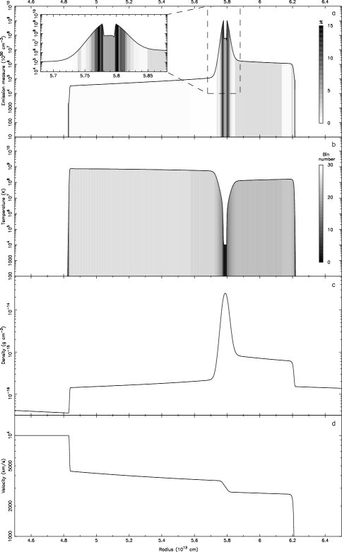
Figure 5.— (a) Emission measure as a function of radius inside the hot shell for run 81 at day 3 after outburst. The data are greyscale coded to represent what percentage of $\text{EM}_{\text{tot}}$ each temperature bin represents. The scaling is shown on the right (ranging $0-15\%$). The inset shows the detail of the region around the contact discontinuity, which provides the majority of $\text{EM}_{\text{tot}}$. The temperature bin in which the post-shock material lies contributes only a very small fraction to $\text{EM}_{\text{tot}}$ (less than 5%). (b) Gas temperature as a function of radius. The data are greyscale coded to represent which of the 30 temperature bins each part of the hot shell belongs to. The lower panels show the gas density (c) and velocity (d) as a function of radius.

The major contribution to the total emission measure is from the region around the contact discontinuity, while the broader forward shocked region with temperatures of $\sim 10^{8}$ K (spanning radii from $5.9-6.2\times 10^{13}$ cm) contributes only a few percent. Orlando et al. (2009) also find in their 3D simulations that most of the X-ray emission originates from a small dense region behind the forward shock. This implies that the total X-ray emission is dominated by material at lower temperatures (around the contact discontinuity) and that the contribution from the hotter forward shocked gas is small. However, the shocked gas might still contribute strongly to the high energy X-rays.

The dot-dash line in the top left panel of Fig. 2 shows the X-ray spectrum emitted by the gas located between the contact discontinuity and the forward shock (we shall call this the post-forward shock gas) with no circumstellar absorption included; the contribution to the total X-ray spectrum is small at low energies but is of the order of 50% for energies above 5 keV. Such a contribution is non-negligible and should have a large impact on the temperature fits to the data. However, the temperature of the emitting gas determines the shape of an X-ray spectrum while the emission measure and distance to the source govern the normalisation of the spectrum.

The post-forward shock gas spectrum is much flatter than the total X-ray spectrum (solid line); by fitting a single temperature MEKAL model to the post-shock gas spectrum at day 3 we obtain $k_{B}T=13.5$ keV, translating as a shock velocity of 3400 km s^-1 which is entirely consistent with the real shock velocity measured in the simulation (black dots in Fig. 4a). This flat post-forward shock spectrum gets drowned by the bright but cooler emission from the rest of the shell which changes the shape of the X-ray spectrum and therefore changes the fit temperature.

Fitting temperatures to the total observed spectra in order to estimate post-shock temperatures and therefore shock velocities is thus unreliable. It also suggests that cosmic ray acceleration at the shock may not be required to explain the discrepancies between velocities derived from observed IR line widths and those derived from X-ray temperature fits (even though such acceleration might still take place).

Finally, the velocity plot in Fig. 5d shows that the material moving at the fast ejection speed of $10^{4}{~{}{\rm km\,s}^{-1}}$ contributes nothing to the X-ray emission and will thus not be observed, while the post reverse shock gas does emit a small amount and its velocities are similar to the ones measured by the IR line widths (as shown in Fig. 4a).

4.4. The RXTE dataset

It has to be noted that even though this study primarily addresses the Swift X-ray data, one cannot ignore the higher energy X-ray data obtained with the RXTE observatory (Sokoloski et al., 2006). There are indeed some differences between the two datasets, taken during the same epoch of the remnant’s evolution. The break in the Swift data around day 7-8 which we interpreted as the end of our fast wind phase (Paper II) is absent from the RXTE data. Instead, a nearly perfect Sedov-Taylor shock deceleration is observed between days 3 and 10 (see Fig. 2b in Sokoloski et al. 2006; note that once again these velocities were computed from single temperature fits to X-ray spectra). The discrepancy between the data is not fully understood. The RXTE probes a higher energy range ($3-20$ keV) than the XRT onboard Swift ($0.3-10$ keV) which would imply that it is sensitive to only the hottest plasma and would therefore give a better estimate of the post-shock temperatures and hence the shock velocities. However, the observed velocities are lower than the velocities derived from Swift observations (Paper I) which is inconsistent with our previous analysis showing that the single temperature fits to the Swift data underestimate the postshock temperatures in the system.

Another important difference between the datasets is that while an increase in total integrated flux is reported for the Swift data between days 3 and 5, a decrease is observed by the RXTE. This can be explained by the fact that a large portion of the energy radiated at day 3 is in the high energy range (thus not well detected by Swift) and then as the blastwave cools adiabatically the radiation moves to lower energies resulting at day 5 in an increase of $5-10$ keV photon counts for Swift and a decrease of $7-20$ keV photon counts for RXTE. In addition, as the forward shock progresses outward clearing the RG wind, the amount of circumstellar absorption reduces which also contributes to an increase of soft X-ray flux. An increase of $3-5$ keV photon counts is observed in the RXTE data which confirms this statement. However, if one compares the same energy band in the two datasets between days 3 and 5, one can see that the X-ray counts between $5-10$ keV increases in the Swift data while it decreases in the RXTE data. Inconsistent datasets will inevitably be difficult to fit with a single model.

The reason why a Sedov-Taylor model fits the early RXTE data and not the Swift is unclear. A general Sedov-Taylor blastwave is produced by an instantaneous release of energy at a point inside an ambient medium with a power-law density profile. No mass is ejected, there is no reverse shock, and the expanding shell is made up only from the ambient gas swept up by the shock. In our model, we have adopted a more physically realistic scenario likely to be applicable to the case of RS Oph where some mass has been ejected in the outburst. Here, the outburst energy is delivered via the kinetic energy of a wind which then interacts with a circumstellar medium with a density described by an inverse-square law as produced by a stellar wind. We have experimented with varying the amounts of outburst energy in kinetic energy or in thermal energy. For example, we have run a simulation using the parameters from run 2 (same $M_{\mathrm{ej}}$ and $E_{0}$) but with half of the outburst energy in thermal form and half in kinetic form. The results are quite different at early times, while remaining very similar at later times ($t>30$ days). At early times, the blastwave expands much faster (due to the instantaneous release of half the outburst energy), the X-ray spectra are much flatter (yielding higher X-ray temperatures) and the velocities are much more Sedov-like. As opposed to the initial run 2, there is a decrease of X-ray flux between days 3 and 5 when folded through both the Swift instrument response and the RXTE response. This is more in line with the RXTE observations but no longer in agreement with the Swift data. A more extreme example injecting 100% of the outburst energy in thermal form (as in the models of O’Brien et al. 1992) also shows a decrease in $5-10$ keV photon counts when folded through the Swift response. We have not been able to obtain results which are consistent with both the Swift and RXTE observations.

5. Conclusions

We have taken the results from our hydrodynamical models described in Paper II and calculated synthetic X-ray spectra using the xspec. The results from runs 1 to 16 of Paper II were first compared to the Swift spectra. It was found that the rate of decrease of the hard X-ray counts was related to the rate of decrease of the forward shock velocities, and a best fitting model would need a relatively low ejecta mass. However, runs with very high ejection velocities $V_{2}$ overestimated the X-ray counts across the spectrum at all times. Run 13 which was thought to be the best fit (based on the forward shock velocities) in Paper II was thus excluded.

A wider exploration of the 1D model parameter space was undertaken to find a model which best fit the observed spectra. A total of 88 runs were carried out, and fluxes were extracted for each day between day 1 and day 100 after outburst for each run. These model fluxes were compared to the fluxes from 70 Swift observational epochs during the same period, being careful to exclude SSS emission as appropriate. Large differences between the observed and theoretical fluxes allowed us to exclude many runs, and the spectra of the few remaining runs with good matching fluxes were examined in order to find a best-fitting model. We are now confident that the mass ejected in the RS Oph outburst is relatively low, around $(2-5)\times 10^{-7}~{}{{\rm M}_{\odot}}$, and that the shock velocities are higher than suggested by X-ray single temperature fits. It was however never possible to simultaneously obtain a sufficiently high level of hard X-ray emission, a flat mid-energy spectrum and an appropriately low level of emission at low energies without including some additional ad-hoc absorption, thus making the derived densities in the RG wind uncertain.

The fast wind velocity of the best-fitting model ($10000{~{}{\rm km\,s}^{-1}}$) is considered unusually high for a nova outburst, but radio observations of O’Brien et al. (2006) and Sokoloski et al. (2008) show evidence for bipolar lobes moving at speeds of the order of $5000{~{}{\rm km\,s}^{-1}}$ at early times ($t<50$ days). Chandra observations of Luna et al. (2009) also report a jet moving at speeds greater than $6000{~{}{\rm km\,s}^{-1}}$. Similarly, Ribeiro et al. (2009) deduce high ejection velocities of $\sim 5100{~{}{\rm km\,s}^{-1}}$ from HST imaging and ground-based optical spectra, albeit the latter two studies are based on observations taken much later (538 and 155 days after outburst, respectively) than the timescales addressed in this paper. Furthermore, the fast ejection velocity may not be easily directly observed as the ejecta are decelerated when they run into the circumstellar medium.

Another important conclusion we can draw from this study is that in the Swift/XRT energy band, the emission from the post-shock material is negligible compared to that of the regions around the high-density contact discontinuity, and that fitting emission models with single temperatures (even when several components with different temperatures are included) to X-ray spectra greatly underestimates immediate post-shock temperatures and hence forward shock velocities. We also showed that velocity estimates from line widths (for example the IR line widths in the case of RS Oph) also underestimate the forward shock velocities.

Some inconsistencies are however present between the Swift and RXTE X-ray datasets, in particular in the forward shock velocities between days 3 and 10. While the spectra of our best fitting model agree well with the Swift observations, they do not fit the RXTE data. This does not affect our results for the subsequent evolution of the remnant (in particular the ejected mass) since RS Oph was very faint in the RXTE energy range after day 10, as opposed to Swift. It just means that the manner in which the mass and energy are ejected during the outburst might be different (for example, the proportions of outburst energy in the form of kinetic and thermal energy may be different).

It has proved difficult to find a set of parameter values for this spherically symmetric model which matches the observed X-ray spectra for all epochs during the first 100 days of the remnant’s evolution. However, radio and optical observations have shown that the remnant of RS Oph has a bipolar morphology. Our suggestion that the additional absorption required to fit the low-energy X-ray spectra might be present in the form of a torus would also fit with an evolving bipolar morphology. Preliminary work on 2D codes with a bipolar ejection is underway, using an equatorial density enhancement in the RG wind. Initial results have shown that is it possible to obtain fast moving material in the polar direction yielding hard X-rays and a high absorption column along the equator at the same time, better resembling the observed X-ray spectra of RS Oph (Vaytet, 2009). A bipolar model might also be able to fit the RXTE observations better if the remnant exhibits more of a Sedov-Taylor blastwave behaviour along one direction. Much work however remains, due to the increasingly large parameter space worthy of exploration.

References

- Abbey et al. (2006) Abbey, A., et al. 2006, in Proc. The X-Ray Universe 2005 (ESA SP-604; Fekel, F. C., Joyce, R. R., Hinkle, K. H., & Skrutskie, M. F. 2000, AJ, 119, 1375 Noordwijk: ESA), 943
- Anupama (2008) Anupama, G. C. 2008, in RS Ophiuchi (2006) and the Recurrent Nova Phenomenon, eds Evans A., Bode M. F., O’Brien T. J., Darnley M. J., ASP Conference Series, 401, 31
- Balman, Krautter & Oegelman (1998) Balman, S., Krautter, J., Oegelman, H. 1998, ApJ, 499, 395
- Barry et al. (2008) Barry, R. K., Mukai, K., Sokoloski, J. L., Danchi, W. C., Hachisu, I., Evans, A., Gehrz, R., Mikolajewska, J. 2008, in RS Ophiuchi (2006) and the Recurrent Nova Phenomenon, eds Evans A., Bode M. F., O’Brien T. J. & Darnley M. J., ASP Conference Series, 401, 52
- Bode (1987) Bode, M. F. 1987, in RS Oph (1985) and the Recurrent Nova Phenomenon, ed. M. F. Bode (Utrecht: VNU Science), 241
- Bode et al. (2006) Bode, M. F. et al. 2006, ApJ, 652, 629 (Paper I)
- Bode et al. (2007) Bode, M. F., Harman, D. J., O’Brien, T. J., Bond, H. M., Starrfield, S., Evans, A., Eyres, S. P. S. 2007, ApJL, 655, L63
- Das et al. (2006) Das, R., Banerjee, D. P. K., Ashok N. M. 2006, ApJL, 653, L141
- Dobrzycka & Kenyon (1994) Dobrzycka, D., Kenyon, S. J. 1994, AJ, 108, 2259
- Evans et al. (2007) Evans, A. et al. 2007, ApJL, 671, L157
- Fekel et al. (2000) Fekel, F. C., Joyce, R. R., Hinkle, K. H, Skrutskie, M. F. 2000, AJ, 119, 1375
- Hachisu et al. (2006) Hachisu, I. et al. 2006, ApJL, 651, L141
- Hachisu et al. (2007) Hachisu, I., Kato, M., Luna, G. J. M. 2007, ApJL, 659, L153
- Hjellming et al. (1986) Hjellming, R. M., van Gorkom, J. H., Seaquist, E. R., Taylor, A. R., Padin, S., Davis, R. J., Bode, M. F. 1986, ApJL, 305, L71
- Krautter et al. (1996) Krautter, J., Oegelman, H., Starrfield, S., Wichmann, R., Pfeffermann, E. 1996, ApJ, 456, 788
- Lloyd et al. (1992) Lloyd, H. M., O’Brien, T. J., Bode, M. F., Predehl, P., Schmitt, J. H. M. M., Truemper, J., Watson, M. G., Pounds, K. A. 1992, Nature, 356, 222
- Luna et al. (2009) Luna, G. J. M., Montez, R., Sokoloski, J. L., Mukai, K., Kastner, J. H. 2009, ApJ, 707, 1168
- Mewe et al. (1986) Mewe, R., Lemen, J. R., van den Oord, G. H. J. 1986, A&AS, 65, 511
- Mukai & Ishida (2001) Mukai, K., Ishida, M. 2001, ApJ, 551, 1024
- Narumi et al. (2006) Narumi, H., Hirosawa, K., Kanai, K., Renz, W., Pereira, A., Nakano, S., Nakamura, Y., Pojmanski, G. 2006, IAUC 8671
- Ness et al. (2009) Ness, J.-U., Drake, J. J., Starrfield, S., Bode, M. F., O’Brien, T. J., Evans, A., Eyres, S. P. S., Helton, L. A., Osborne, J. P., Page, K. L., Schneider, C., Woodward, C. E. 2009, AJ, 137, 3414
- O’Brien et al. (2008) O’Brien, T. J., Beswick, R. J., Bode, M. F., Eyres, S. P. S., Muxlow, T. W. B., Garrington, S. T., Porcas, R. W., Evans, A., Davis, R. J., 2008, in RS Ophiuchi (2006) and the Recurrent Nova Phenomenon, eds Evans A., Bode M. F., O’Brien T. J. & Darnley M. J., ASP Conference Series, 401, 239
- O’Brien et al. (1992) O’Brien, T. J., Bode, M. F., Kahn, F. D. 1992, MNRAS, 255, 683
- O’Brien et al. (2006) O’Brien, T. J., Bode, M. F., Porcas, R. W., Muxlow, T. W. B., Eyres, S. P. S., Beswick, R. J., Garrington, S. T., Davis, R. J., Evans, A. 2006, Nature, 442, 279
- O’Brien et al. (1994) O’Brien, T. J., Lloyd, H. M., Bode, M. F. 1994, MNRAS, 271, 155
- Oppenheimer & Mattei (1993) Oppenheimer, B. D., Mattei, J. A. 1993, JAAVSO, 22, 105
- Orlando et al. (2009) Orlando, S., Drake, J. J., Laming, J. M. 2009, A&A, 493, 1049
- Osborne et al. (2006) Osborne, J. P. et al. 2006, Astronomer’s Telegram 770
- Osborne et al. (2011) Osborne, J. P. et al. 2008, ApJ, 727, 124
- Page et al. (2008) Page, K. L., Osborne, J. P., Beardmore, A. P., Goad, M. R., Wynn, G. A., Bode, M. F., O’Brien, T. J. 2008, in RS Ophiuchi (2006) and the Recurrent Nova Phenomenon, eds Evans A., Bode M. F., O’Brien T. J. & Darnley M. J., ASP Conference Series, 401, 283
- Ribeiro et al. (2009) Ribeiro, V. A. R. M., et al. 2009, ApJ, 703, 1955
- Rosino (1987) Rosino, L. 1987, in RS Oph (1985) and the Recurrent Nova Phenomenon, ed. M. F. Bode (Utrecht: VNU Science), 1
- Rosino & Iijima (1987) Rosino, L., Iijima, T. 1987, in RS Oph (1985) and the Recurrent Nova Phenomenon, ed. M. F. Bode (Utrecht: VNU Science), 27
- Rupen et al. (2008) Rupen, M. P., Mioduszewski, A. J., Sokoloski, J. L. 2008, ApJ, 688, 559
- Schaefer (2004) Schaefer, B. 2004, IAUC, 8396
- Schaefer (2009) Schaefer, B. 2009, ApJ, 697, 721
- Sokoloski et al. (2006) Sokoloski, J. L., Luna, G. J. M., Mukai, K., Kenyon, S. J. 2006, Nature, 442, 276
- Sokoloski et al. (2008) Sokoloski, J. L., Rupen, M. P., Mioduszewski, ApJL, 2008, 685, L137
- Starrfield (2008) Starrfield, S. 2008, in Classical Novae, eds Bode M. F. & Evans A., Wiley, Cambridge University Press, Second edition, Chapt. 4
- Tatischeff & Hernanz (2008) Tatischeff, V., Hernanz, M. 2008, in RS Ophiuchi (2006) and the Recurrent Nova Phenomenon, eds Evans A., Bode M. F., O’Brien T. J., Darnley M. J., ASP Conference Series, 401, 332
- Vaytet (2009) Vaytet, N. M. H. 2009, PhD Thesis, The University of Manchester
- Vaytet et al. (2007) Vaytet, N. M. H., O’Brien, T. J., Bode, M. F., 2007, ApJ, 665, 654 (Paper II)
- Walder et al. (2008) Walder, R., Folini, D., Shore, S. N. 2008, A&AL, 484, L9
- Wilms et al. (2000) Wilms, J., Allen, A., McCray, R., 2000, ApJ, 542, 914
- Yaron et al. (2005) Yaron, O., Prialnik, D., Shara, M. M., Kovetz, A., 2005, ApJ, 623, 398