The effect of radiative gravitational modes on the dynamics of a cylindrical shell of counter rotating particles

Abstract

In this paper we consider some aspects of the relativistic dynamics of a cylindrical shell of counter rotating particles. In some sense these are the simplest systems with a physically acceptable matter content that display in a well defined sense an interaction with the radiative modes of the gravitational field. These systems have been analyzed previously, but in most cases resorting to approximations, or considering a particular form for the initial value data. Here we show that there exists a family of solutions where the space time inside the shell is flat and the equation of motion of the shell decouples completely from the gravitational modes. The motion of the shell is governed by an equation of the same form as that of a particle in a time independent one dimensional potential. We find that under appropriate initial conditions one can have collapsing, bounded periodic, and unbounded motions. We analyze and solve also the linearized equations that describe the dynamics of the system near a stable static solutions, keeping a regular interior. The surprising result here is that the motion of the shell is completely determined by the configuration of the radiative modes of the gravitational field. In particular, there are oscillating solutions for any chosen period, in contrast with the “approximately Newtonian plus small radiative corrections” motion expectation. We comment on the physical meaning of these results and provide some explicit examples. We also discuss the relation of our results to the initial value problem for the linearized dynamics of the shell.

I Introduction

In this paper we consider some aspects of the relativistic dynamics of a cylindrical shell of counter rotating particles. In some sense these are the simplest systems with a physically acceptable matter content that display in a well defined sense an interaction with the radiative modes of the gravitational field. The dynamics of these systems was analyzed originally by Apostolatos and Thorne apostol , but the evolution was considered in detail only over very short periods of time, and imposing a particular form for the initial data, the “momentarily static radiation free” (MSRF) form note1 , and the question of the general evolution in time of the system has remained largely unexplored. We notice that most of the literature that followed the work Apostolatos and Thorne has concentrated in the problem of collapse (see, for instance, goncalves and wang ), and in general imposing particular forms for the fields, that may include also some form of non gravitational radiation outside the shell (see, for instance, pereira , gleiser or seriru ). In a recent paper Hamity, Barraco and Cécere hamity , have considered again the relativistic dynamics of these systems. In particular, since the system may have stable static configuration, and in the Newtonian limit small departures form the static configuration lead to periodic motions, it was expected that in the fully relativistic dynamics the inclusion of gravitational radiation modes should lead to a damping of these oscillations, through some form of “radiation reaction”. This expectation appears to be satisfied in the numerical solutions obtained in hamity . A closer analysis reveals, however, that the authors assumed an approximation where the back reaction of the radiative modes is essentially disregarded. This approximation would be justified if the coupling to the gravitational radiation modes had only a small effect on the dynamics of the shell. It turns out, however, as is shown in the present paper, that rather the opposite situation holds, and the dynamics is completely dominated by the behaviour of these modes. In fact we find that, in some sense, the coupling of the shell to the gravitational radiation modes is as strong as it can be, a remarkable fact that shows the dynamics of this system cannot be approximated by a Newtonian dynamics plus post - Newtonian corrections, as in the case of models where matter is confined to a bounded region.

The plan of the paper is as follows. After setting up the problem in Section II, we show in Section III that there exists a family of solutions where the space time inside the shell is flat and the equation of motion of the shell decouples completely from the gravitational modes. The motion of the shell is governed by an equation of the same form as that of a particle in a time independent one dimensional potential. We find that under appropriate initial conditions one can have collapsing, bounded periodic, or unbounded motions. Next, in Section V we analyze the linearized equations that describe the dynamics of the system near a stable static solutions, keeping a regular interior. The surprising result here is that the motion of the shell is completely determined by the configuration of the radiative modes of the gravitational field. In particular, there are oscillating solutions for any chosen period, in contrast with the “approximately Newtonian plus small radiative corrections” motion expectation. Another interesting modes that appear here are the “anti resonances” discussed in Section VI. In Section VII we consider the general behaviuor of the periodic solutions, and in Section VIII their relation to the initial value problem for the linearized dynamics of the shell. We comment on the physical meaning of these results and provide some explicit examples. We also consider the role of the momentarily static and radiation free initial data of apostol , in this context. Some closing comments are contained in Section IX.

II Equations of motion

We consider a spacetime $M=M^{-}\cup\Sigma\cup M^{+}$ ($M^{-}$ and$M^{+}$ are manifolds with boundary where the boundaries are identified with the 3-manifold $\Sigma$) with cylindrical symmetry where $\Sigma$ is the history of a hollow cylinder composed of counter-rotating particles of rest mass equal to unity; $M^{-}(M^{+})$ is the vacuum interior (exterior) region of the cylinder. In the vacuum interior $(M^{-})$ and exterior $(M^{+})$ of the shell, we introduce canonical cylindrical coordinates $(t,r,z,\phi)$. The metric takes the form apostol .

$$ds^{2}_{\pm}=e^{2\gamma_{\pm}-2\psi_{\pm}}\left(dr^{2}-dt^{2}_{\pm}\right)+e^{2\psi_{\pm}}dz^{2}+e^{-2\psi_{\pm}}r^{2}d\phi^{2}$$ (1)

Dropping the $\pm$ indices, the Einstein field equations in the empty space inside and outside the shell are,

$$\psi_{,rr}+\frac{1}{r}\psi_{,r}-\psi_{,tt}=0$$ (2)

$$\gamma_{,t}=2r\psi_{,r}\psi_{,t}\;\;\;,\;\;\;\gamma_{,r}=r\left[(\psi_{,r})^{2}+(\psi_{,t})^{2}\right]$$ (3)

We may interpret $\psi(r,t)$ as playing the role of a gravitational field whose static part is the analogue of the Newtonian potential. The time dependent solutions of (2) represent gravitational waves ER . Equation (2) is the integrability condition of Eqs. (3). The coordinates $(z,\phi,r)$ and the metric function $\psi$ are continuous across the shell $\Sigma$, while $t$ and the metric function $\gamma$ are discontinuous. Smoothness of the spacetime geometry on the axis $r=0$ requires that $\gamma=0$ and $\psi$ finite at $r=0$. The junction conditions of $M^{-}$ and $M^{+}$ through $\Sigma$ require the continuity of the metric and specify the jump of the extrinsic curvature $K^{\pm}$ compatible with the stress energy tensor on the shell. The induced metric on $\Sigma$ is given by

$$ds^{2}_{\Sigma}=-d\tau^{2}+e^{2\psi_{\Sigma}}dz^{2}+e^{-2\psi_{\Sigma}}R^{2}d\phi^{2}$$ (4)

Here $\psi_{\Sigma}(\tau)=\psi_{+}(R(\tau),t_{+}(\tau))=\psi_{-}(R(\tau),t_{-}(\tau))$. The evolution of the shell is characterized by $R(\tau)$, which is the radial coordinate $r$ at the shell’s location and $\tau$ the proper time of an observer at rest on $\Sigma$. If we assume, as in apostol , and hamity , that the shells is made up of equal mass counter rotating particles, the Einstein field equations on the shell may be put in the form,

$$\psi^{+}_{,n}-\psi^{-}_{,n}=-\frac{2\lambda}{\sqrt{R^{2}+e^{2\psi_{\Sigma}}J^{2}}}$$ (5)

$$X^{+}-X^{-}=-\frac{4\lambda\sqrt{R^{2}+e^{2\psi_{\Sigma}}J^{2}}}{R}$$ (6)

where the constants $\lambda$ and $J$ are, respectively, the proper mass per unit Killing length of the cylinder and the angular momentum per unit mass of the particles. The other quantities in (5,6) are given by,

$$X^{\pm}\equiv\frac{\partial t_{\pm}}{\partial\tau}=+\sqrt{e^{-2(\gamma_{\pm}-\psi_{\Sigma})}+\dot{R}^{2}}$$ (7)

$$\psi^{\pm}_{,n}=\psi^{\pm}_{,r}X^{\pm}+\psi^{\pm}_{,t}\dot{R}$$ (8)

where a dot indicates a $\tau$ derivative, and we also have,

$$\frac{d^{2}R}{d\tau^{2}} = \dot{R}\dot{\psi_{\Sigma}}-R\left[(\dot{\psi_{\Sigma}})^{2}+(\psi^{-}_{,n})^{2}\right]$$ (9)

$$+\frac{R^{2}\psi^{-}_{,n}X^{-}}{R^{2}+e^{2\psi_{\Sigma}}J^{2}}-\frac{\lambda R^{2}X^{-}}{(R^{2}+e^{2\psi_{\Sigma}}J^{2})^{3/2}}+\frac{J^{2}e^{2\psi_{\Sigma}}X^{-}X^{+}}{R(R^{2}+e^{2\psi_{\Sigma}}J^{2})}$$

Equations (5,6,9), together with (2,3) determine the evolution of the shell and of the gravitational field to which it is coupled. The relevant functions: $R(\tau)$, $\psi_{\pm}(r,t_{\pm})$, and $\gamma_{\pm}(r,t_{\pm})$ appear satisfying a rather complex set of coupled ordinary and partial differential equations, with the boundary values for $\psi_{\pm}$ and $\gamma_{\pm}$ at $t=t_{\pm}(\tau),r=R(\tau)$ directly coupled to the motion of the shell. Because of this complexity, the system was first analyzed in apostol only to show some properties of the motion, although no solution was obtained, and later in hamity , where, after introducing a second shell, mainly for technical reasons, an approximation that leads to an effective decoupling of (9) was used, to avoid considering the complex boundary problem that results for the wave equations (2) for $\psi_{\pm}$. Some full solutions of the problem are considered in the following Sections.

III A restricted set of solutions

A full solution of the problem should provide the evolution of arbitrary initial data, satisfying the constraints imposed by the field equations. This is, clearly, a very complex problem. There is, however, a restriction on the set of solutions that while retaining its most interesting feature, namely, the coupling of the shell with radiative modes of the gravitational field, still simplifies considerably the system, allowing for a complete analysis of the resulting evolution and of its physical meaning.

III.1 Static solutions

We will first consider the static solutions for a shell of constant radius $R$, assuming an empty flat interior apostol , hamity . In this case we may take $\gamma_{-}=0$, $\psi_{-}=0$, implying $\psi_{\Sigma}=0$, and for the exterior field we have,

$$\psi^{+}(r)=-\kappa\ln(r/R)\;\;\;,\;\;\;\gamma^{+}(r)=\gamma_{0}+\kappa^{2}\ln(r/R)$$ (10)

then,

$$X^{+}(r)=e^{-\gamma_{0}}\;\;\;,\;\;\;X^{-}=1$$ (11)

Since $\dot{R}=0$, $\dot{\psi}_{\Sigma}=0$, and $\psi^{-}_{,n}=0$, we find,

$$\kappa=2\frac{J^{2}}{R^{2}}\;\;\;,\;\;\;\gamma_{0}=2\ln\left[(R^{2}+2J^{2})/R^{2}\right]$$ (12)

and,

$$\lambda=\frac{J^{2}R\sqrt{J^{2}+R^{2}}}{(2J^{2}+R^{2})^{2}}$$ (13)

This means that for any static solution we must have $\lambda\leq 0.15879...$, (see hamity ).

III.2 Non static solutions with a flat interior

The previous results indicate that, at least for the static case, we have solutions where the interior region of the shell is empty and flat. We notice that for a similar problem, namely a shell of counter rotating particles, but with spherical symmetry, we may have non static solutions where the radius of the shell changes in time, but the interior remains flat. In this case the spherical symmetry is crucial, as this implies that there are no radiative modes for the gravitational field. This is not the case for cylindrical symmetry, and, in general, one does not expect that in the non static case the interior will remain flat, because radiative gravitational modes, corresponding to a non static $\psi$, will in general penetrate the interior region for, otherwise, the matching conditions would not be satisfied. Nevertheless, given the existence of the static solution with an empty flat interior, it is worthwhile to explore to what extent, if any, this condition can be generalized to a non static solution. We, therefore, assume again $\gamma_{-}=0$, $\psi_{-}=0$, (implying $\psi_{\Sigma}=0$, $\psi^{-}_{,n}=0$, and $X^{-}=\sqrt{1+(\dot{R})^{2}}$ ), but place no restriction on either $R(\tau)$ or $\psi_{+}$, and $\gamma_{+}$. The field equations are now (2), (3), and on the shell we have,

$$X^{+}=\sqrt{1+(\dot{R})^{2}}-\frac{2\lambda}{\sqrt{R^{2}+J^{2}}}$$ (14)

Using this, and the fact that $\dot{\psi}_{\Sigma}=0$, we find,

$$\frac{d^{2}R}{d\tau^{2}}=\frac{(1+(\dot{R})^{2})J^{2}}{R(R^{2}+J^{2})}-\frac{\sqrt{1+(\dot{R})^{2}}(R^{2}+2J^{2})^{2}\lambda}{R^{2}(R^{2}+J^{2})^{3/2}}$$ (15)

The first surprising thing about this equation is that it contains no information on $\psi$, and, therefore, it is an autonomous equation, completely decoupled from the gravitational mode. Equally unexpected is that it admits a simple first integral, given by,

$$C=-\frac{\lambda}{2}\ln\left({R}^{2}+{J}^{2}\right)+2\,{\frac{\lambda\,{J}^{2}}{{R}^{2}}}-{\frac{\sqrt{{R}^{2}+{J}^{2}}}{R}}\sqrt{\left(\frac{dR}{d\tau}\right)^{2}+1},$$ (16)

where $C$ is a constant. This may also be written in the form

$$\left(\frac{dR}{d\tau}\right)^{2}+1-\frac{\left[4\lambda J^{2}-\lambda R^{2}\ln(R^{2}+J^{2})-2CR^{2}\right]^{2}}{4R^{2}(R^{2}+J^{2})}=0,$$ (17)

and, therefore, the motion of the shell is identical to that of a particle of unit mass in the potential,

$$V(R)=\frac{1}{2}\left[1-\frac{\left[4\lambda J^{2}-\lambda R^{2}\ln(R^{2}+J^{2})-2CR^{2}\right]^{2}}{4R^{2}(R^{2}+J^{2})}\right]$$ (18)

with vanishing total energy. Notice that $C$ is not this energy and, therefore, the form of $V(R)$ will be different for different solutions. Nevertheless, (17) implies that if there are suitable choices of the parameters for which the potential $V(r)$ has a negative minimum, the shell may execute a periodic motion. Let us first find the conditions under which this may happen. We look for equilibrium points (static solutions) where $\dot{R}=0$, and $\ddot{R}=0$. Let $R=R_{0}$ be that point, then, from (15), we have,

$$\lambda=\frac{J^{2}R_{0}\sqrt{R_{0}^{2}+J^{2}}}{(R_{0}^{2}+2J^{2})^{2}}$$ (19)

which may also be considered as an equation for $R_{0}$, given $\lambda$ and $J$,

To check for stable equilibrium points we set $R(\tau)=R_{0}+\xi(\tau)$, replace in (15), and expand to first order in $\xi(\tau)$. We find,

$$\frac{d^{2}\xi}{d\tau^{2}}=-\frac{[2R_{0}^{4}-(R_{0}^{2}+2J^{2})J^{2}]J^{2}}{R_{0}^{2}(R_{0}^{2}+J^{2})^{2}(R_{0}^{2}+2J^{2})}\xi$$ (20)

Then, the static solution will be stable for $R_{0}^{2}/J^{2}>(1+\sqrt{17})/4$, ($R_{0}/J>1.1317...$) and unstable otherwise (see also hamity ).

The somewhat complex form and dependence on its parameters of $V(R)$ makes a general analysis of the possible motions based on (17) rather difficult. We notice, however, that we have,

$$V(R)=-(\lambda\ln(R)+C)^{2}/2+{\cal{O}}(R^{0})\;\;\;,\;\;\;R\to\infty$$ (21)

and

$$V(R)=-2\lambda^{2}R^{-2}+{\cal{O}}(R^{0})\;\;\;,\;\;\;R\to 0$$ (22)

and therefore we have unbounded motions for sufficiently large $R$ and collapsing motions for sufficiently small $R$. Moreover, the equation,

$$4\lambda J^{2}-\lambda R^{2}\ln(R^{2}+J^{2})-2CR^{2}=0$$ (23)

has a real root with $R=R_{m}>0$ for any real $J$ and $C$, and $\lambda>0$. But for $R=R_{m}$ we have $V(R)=1/2$, which is also the maximum possible value of $V(R)$, and, therefore, the collapsing and unbounded motion regions are separated at least by a ”forbidden” gap. Depending on the values of the parameters, $V(r)$ may contain two ”forbidden” gaps, where $V(r)>0$, and periodic motions are possible in the region between these gaps. Figure 1 provides some explicit examples of these cases. They will be explored in more detail in the next Sections.

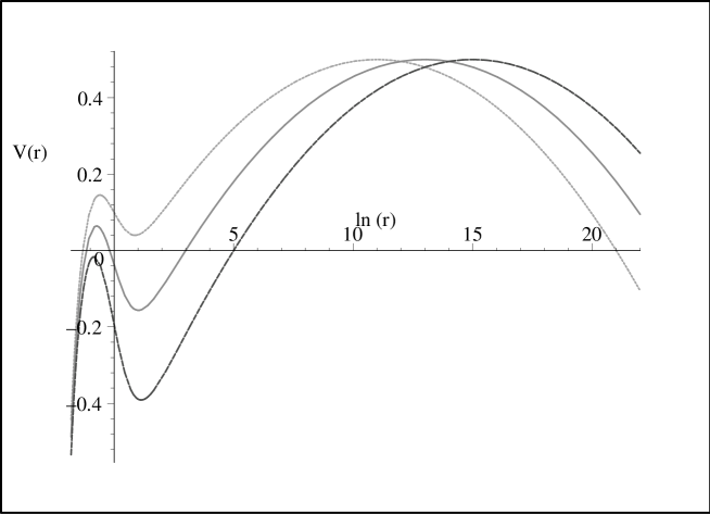
Figure 1: Plots of $V(r)$ as a function of $\ln(r)$. We have taken $J=1$, and $\lambda=0.1$ in all cases. The solid curve, for $C=-1.3$, contains a region where periodic motions are possible. This region is absent for both the dotted ($C=-1.1$), and the dashed ($C=-1.5$) curves. In all cases we have a collapsing region, for sufficiently small $r$, and unbounded region, for sufficiently large $r$.

To close this Subsection we remark also that the evolution equation (15) has the following scaling property: if we introduce the function $\tilde{R}(\eta)$, such that,

$$\tilde{R}(\eta)\equiv\frac{1}{J}R(J\eta)$$ (24)

we have

$$\frac{d^{2}\tilde{R}}{d{\eta}^{2}}+{\frac{\sqrt{\left({\frac{d\tilde{R}}{d\eta}}\right)^{2}+1}\left(\tilde{R}^{2}+2\right)^{2}\lambda}{\left(\tilde{R}^{2}+1\right)^{3/2}\tilde{R}^{2}}}-{\frac{\left({\frac{d\tilde{R}}{d\eta}}\right)^{2}+1}{\tilde{R}\left(\tilde{R}^{2}+1\right)}}=0$$ (25)

and, therefore, all the types of motions, up to scalings, are determined by the (adimensional) parameter $\lambda$.

III.3 Compatibility with the field equations

So far we have only considered Eq. (15). The full set of field equations includes also $\psi$, $\gamma$ and the junction conditions, and there is, a priori, no guarantee that the only solutions of (15) compatible with these are the static ones. In particular, the condition $\psi_{\Sigma}=0$ implies,

$$\psi^{+}_{,r}(R(\tau),t^{+}(\tau))\dot{R}+\psi^{+}_{,t}(R(\tau),t^{+}(\tau))X^{+}=0$$ (26)

which, together with (8), and (14), determine $\psi^{+}_{,r}(R(\tau),t^{+}(\tau))$ and $\psi^{+}_{,t}(R(\tau),t^{+}(\tau))$ in terms of $R(\tau)$. After some simplifications, and using (17), we find,

$$\psi^{+}_{,r}(R(\tau),t^{+}(\tau)) = -\frac{\lambda[4\lambda J^{2}+8\lambda R^{2}+\lambda R^{2}\ln(R^{2}+J^{2})+2CR^{2}]}{R(R^{2}+J^{2})[1+4\lambda^{2}\ln(R^{2}+J^{2})+8\lambda C+16\lambda^{2}]}$$

$$\psi^{+}_{,t}(R(\tau),t^{+}(\tau)) = \frac{2\lambda\dot{R}}{\sqrt{R^{2}+J^{2}}[1+4\lambda^{2}\ln(R^{2}+J^{2})+8\lambda C+16\lambda^{2}]}$$ (27)

Similarly, from (14), we have,

$$\gamma^{+}(R(\tau),t^{+}(\tau))=-\frac{1}{2}\ln[1+4\lambda^{2}\ln(R^{2}+J^{2})+8\lambda C+16\lambda^{2}]$$ (28)

From this equation we may compute,

$$\frac{d\gamma^{+}}{d\tau}=\gamma^{+}_{,r}\dot{R}+\gamma^{+}_{,t}X^{+}$$ (29)

and we can check that if we replace (3) on the right, and then use (III.3), we get the same expression as that obtained by computing the left hand side of (29) using (28). We conclude that the restriction to a flat interior is compatible with the dynamics of $\gamma$ on the shell, even in the non stationary case.

Now we could compute in principle $\psi$ (and then $\gamma$) outside the shell. We notice that, provided $R(\tau)$ satisfies some suitable conditions, to be considered below, if we only imposed $\psi_{\Sigma}=0$, since $R(\tau)$ is given, then we would get for $\psi$ a wave equation with a well defined boundary condition . But in this case both $\psi_{,r}$ and $\psi_{,t}$ are given in the boundary, and it is not clear that in this case we may get any non trivial solution. To analyze this problem we notice that in (2) we may consider $r$ as the “time” variable, and $t$ as the “space” variable reula , as shown in Figure 2. Then, the problem can be posed as that of finding the evolution (in $r$) of $\psi$, for initial data ($\psi_{\Sigma}=0,\psi_{,r}$) on the (one dimensional) surface ${\cal{S}}$,

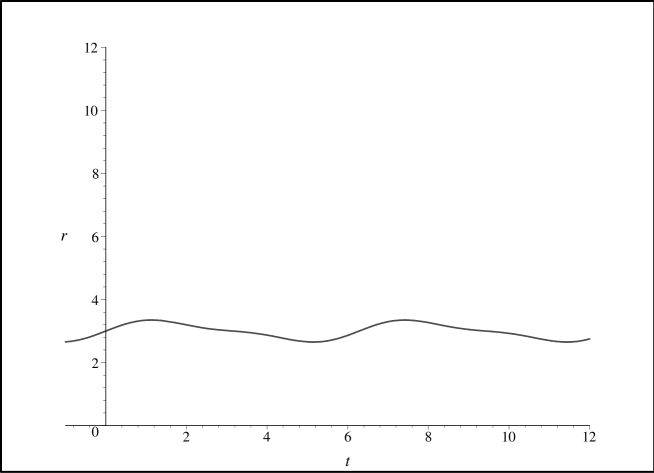
Figure 2: Evolving $\psi_{+}(t,r)$ from “initial data” $(\psi=0,\psi_{,r})$ on the curve $(r=R(\tau),t=t_{+}(\tau))$, represented by the thick curve in the Figure. $\psi_{+}(t,r)$ is evolved into the region above this curve.

$$t=\eta\;\;\;,\;\;\;r=R(\tau(\eta))$$ (30)

where $\eta$ is a parameter, and $\tau(t)$ is obtained by inverting (14). The problem is well posed provided that ${\cal{S}}$ is a Cauchy surface, and this requires that the tangent vector to ${\cal{S}}$ be “space like”, that is, $(dt/d\eta)^{2}-(dr/d\eta)^{2}>0$, or

$$\left(X^{+}\right)^{2}>(\dot{R})^{2}$$ (31)

But, from (7), this is always satisfied. We might, therefore, conclude that the field equations have solutions for any $R(\tau)$ that is a solution of (15). However, we must also require that the data $\psi_{,r}(R(\tau))$ be non singular, but, as can be seen from (III.3), this may not always be the case, because the factor $[1+4\lambda^{2}\ln(R^{2}+J^{2})+8\lambda C+16\lambda^{2}]$ in the denominator in (III.3) may vanish for some finite $R\neq 0$. We notice here that solving (23) for $\ln(R_{m}^{2}+J^{2})$ we get,

$$1+4\lambda^{2}\ln(R_{m}^{2}+J^{2})+8\lambda C+16\lambda^{2}=1+16\,{\frac{\left({R_{{m}}}^{2}+{J}^{2}\right){\lambda}^{2}}{{R_{{m}}}^{2}}}$$ (32)

Since the left hand side is a monotonically increasing function of $R$, this implies that the denominator is always positive for $R>R_{m}$, and, therefore, this problem does not arise for the unbounded solutions of the previous Subsection. Periodic motions are only possible if the potential has, besides that for $R=R_{m}$ with $V(R_{m})=1/2$, another maximum for say $R=R_{p}$, with $V(R_{p})>0$. For this maximum we would have,

$$\left.\frac{dV}{dR}\right|_{R=R_{p}}=-\left.\frac{F_{1}F_{2}}{4R^{3}(R^{2}+J^{2})^{2}}\right|_{R=R_{p}}=0$$ (33)

where,

$$F_{1}=\lambda R^{2}\ln(R^{2}+J^{2})+2CR^{2}-4\lambda J^{2}$$ (34)

and,

$$F_{2}={R}^{2}\lambda\,\ln\left({R}^{2}+{J}^{2}\right){J}^{2}+2\,\lambda\,\left(2\,{J}^{4}+{R}^{4}\right)+2\,{R}^{2}{J}^{2}\left(C+4\,\lambda\right)$$ (35)

The first factor in (33), $F_{1}$, vanishes for $R=R_{m}$. We can check that this is its only zero for $R>0$ by noticing that,

$$\left.\frac{dF_{1}}{dR}\right|_{R=R_{m}}=2\,{\frac{\lambda\,\left({R_{m}}^{2}+2\,{J}^{2}\right)^{2}}{R_{m}\left({R_{m}}^{2}+{J}^{2}\right)}}>0$$ (36)

and, therefore, the equation $F_{1}=0$ can have only one root for $R>0$. Then, any extremum of $V(R)$ other than that for $R=R_{m}$ must come from the vanishing of the second factor, $F_{2}$. It can be shown that $F_{2}$ can have zero, one or two roots depending on the parameters and that each root $R_{p}$ must satisfy $R_{p}<R_{m}$. If $F_{2}$ has no root or only one, $V(r)$ has only one maximum (at $R_{m}$, the root of $F_{2}$ being a saddle point) and there are no periodic motions. If $F_{2}$ has two roots, $V(r)$ has two maxima and a minimum between them (a maximum and a minimum at the roots of $F_{2}$ and another maximum at $R_{m}$). In this case we can have periodic motions only if $V>0$ at the first maximum and $V<0$ at the minimum, and this depends non trivially on the choice of parameters. We can, nevertheless, obtain a useful result as follows. At a root $R_{p}$ of $F_{2}$ we have,

$$\ln\left({R_{{p}}}^{2}+{J}^{2}\right)=-2{\frac{2\,{J}^{4}+{R_{{p}}}^{4}+4{R_{{p}}}^{2}{J}^{2}}{{R_{{p}}}^{2}{J}^{2}}}-2{\frac{C}{\lambda}}$$ (37)

and, therefore, we may write,

$$V(R_{p})=\frac{1}{2}\left(1-\frac{\lambda^{2}(R_{p}^{2}+2J^{2})^{4}}{J^{4}R_{p}^{2}(R_{p}^{2}+J^{2})}\right)$$ (38)

Then, if $V(R_{p})$ is a positive maximum we must have,

$${\lambda}^{2}={\frac{\eta\,{J}^{4}{R_{p}}^{2}\left({R_{p}}^{2}+{J}^{2}\right)}{\left({R_{p}}^{2}+2\,{J}^{2}\right)^{4}}}$$ (39)

with $0\leq\eta<1$. Replacing in the problematic factor in the denominator of (III.3) we have,

$$1+4{\lambda}^{2}\ln\left({R_{p}}^{2}+{J}^{2}\right)+8C\lambda+16{\lambda}^{2}=1-8{\frac{{J}^{2}\left({R_{p}}^{2}+{J}^{2}\right)\left({R_{p}}^{4}+2{R_{p}}^{2}{J}^{2}+2{J}^{4}\right)\eta}{\left({R_{p}}^{2}+2{J}^{2}\right)^{4}}}$$ (40)

The right hand side of (40) is a linear function of $\eta$. It is equal to $1$ for $\eta=0$ and to ${R_{p}}^{8}/({R_{p}}^{2}+{J}^{2})^{4}$ for $\eta=1$. Since the left hand side of (40) is a monotonic function of $R$, it is positive at any positive maximum of $V(R)$ and the oscillating solutions always take place at $R>R_{p}$ (after the first positive maximum), we conclude that (III.3) is well defined and finite for any periodic motion.

As indicated, there are also collapsing solutions with a flat interior. In this case we find that ${\psi^{+}}_{,r}(R(\tau),t^{+}(\tau))$ is singular either at some finite $R$ or at $R=0$. It can be checked that these singularities occur for finite $\tau$ and $t^{\pm}$. Since the solutions are symmetric in $\tau$, this implies that the evolution has singularities both at some finite time in the past and in the future, and, therefore, by causality they extend only to some bounded region in $r$. We do not analyze further these solutions as they do not seem to be physically interesting.

In the following Sections we consider linearized solutions corresponding to infinitesimally small departures from the static stable solutions, both for flat and for empty regular interiors.

IV Linearized periodic solutions with a flat interior

Let us assume that $R=R_{0}$ corresponds, for some suitable $J$, to a stable static solution with $\lambda$ given by (19). For this solution we have $\psi_{-}=0$, $\psi_{\Sigma}=0$, and $\gamma_{-}=0$, with $\psi_{+}$ and $\gamma_{+}$ given by (10,12). We consider now a perturbation of the static solution such that the interior remains flat. This means that we keep $\psi_{-}=0$, $\psi_{\Sigma}=0$, and $\gamma_{-}=0$, but for the other dynamic variables we introduce now a time dependence by setting,

$$R(\tau) = R_{0}+\xi(\tau)$$

$$\psi_{+}(r,t_{+}) = -\kappa\ln(r/R_{0})+\bar{\psi}(r,t_{+})$$ (41)

$$\gamma_{+}(r,t_{+}) = \gamma_{0}+\kappa^{2}\ln(r/R_{0})+\bar{\gamma}(r,t_{+})$$

with $\kappa$ and $\gamma_{0}$ given by (12) with $R=R_{0}$, and consider the linearized field equations that result from expanding to first order in $\xi$, $\bar{\psi}$ and $\bar{\gamma}$. To this order $\xi$ satisfies (20). If we define,

$$\Omega^{2}_{0}=\frac{[2R_{0}^{4}-(R_{0}^{2}+2J^{2})J^{2}]J^{2}}{R_{0}^{2}(R_{0}^{2}+J^{2})^{2}(R_{0}^{2}+2J^{2})}$$ (42)

the solution of (20) can be written as,

$$\xi(\tau)=\xi_{0}e^{i\Omega_{0}\tau}$$ (43)

In accordance with (7), and (14), and expanding to first order in $\xi_{0}$, we have,

$$\frac{dt_{+}}{d\tau}=\frac{R_{0}^{4}}{(R_{0}^{2}+2J^{2})^{2}}+\frac{4J^{4}\xi_{0}e^{i\Omega_{0}\tau}}{(R_{0}^{2}+2J^{2})^{2}R_{0}}$$ (44)

Actually, the last term on the right in (44) contributes in all relevant equations only to second order, and, therefore, we may set,

$$t_{+}=\frac{R_{0}^{4}}{(R_{0}^{2}+2J^{2})^{2}}\tau$$ (45)

when appropriate. Similarly, we may set $t_{-}=\tau$. We also define, for convenience,

$$\Omega_{2}=\frac{(R_{0}^{2}+2J^{2})^{2}}{R_{0}^{4}}\Omega_{0}$$ (46)

We look now for solutions of $\psi$ and $\gamma$ with the same periodicity as $R(\tau)$. On account of (2) and (45) the general solution for $\psi$ will be then of the form,

$$\psi_{+}(t_{+},r)=-\frac{2J^{2}}{R_{0}^{2}}\ln\left(\frac{r}{R_{0}}\right)+\left(A_{2}J_{0}(\Omega_{2}r)+B_{2}Y_{0}(\Omega_{2}r)\right)e^{i\Omega_{2}t_{+}}$$ (47)

where $A_{2}$ and $B_{2}$ are constants, and $J_{0}$, and $Y_{0}$ are Bessel functions. Then the junction conditions on the shell, and the condition $\psi_{\Sigma}=0$ are satisfied (to first order in $\xi_{0}$) if,

$$A_{2} = -\pi J^{2}\left[\frac{J^{2}(4J^{2}R_{0}^{2}+4J^{4}-R_{0}^{4})}{(R_{0}^{2}+J^{2})R_{0}^{7}}Y_{0}(\Omega_{2}R_{0})+\frac{\Omega_{0}(R_{0}^{2}+2J^{2})^{2}}{R_{0}^{6}}Y_{1}(\Omega_{2}R_{0})\right]\xi_{0}$$

$$B_{2} = \pi J^{2}\left[\frac{J^{2}(4J^{2}R_{0}^{2}+4J^{4}-R_{0}^{4})}{(R_{0}^{2}+J^{2})R_{0}^{7}}J_{0}(\Omega_{2}R_{0})+\frac{\Omega_{0}(R_{0}^{2}+2J^{2})^{2}}{R_{0}^{6}}J_{1}(\Omega_{2}R_{0})\right]\xi_{0}$$ (48)

Similarly, again to first order in $\xi_{0}$, we find

$$\gamma_{+}(t_{+},r)=\gamma_{0}+\frac{4J^{4}}{R_{0}^{4}}\ln\left(\frac{r}{R_{0}}\right)-\frac{4J^{2}}{R_{0}^{2}}\left(A_{2}J_{0}(\Omega_{2}r)+B_{2}Y_{0}(\Omega_{2}r)\right)e^{i\Omega_{2}t_{+}}$$ (49)

where,

$$\gamma_{0}=\ln\left[\frac{(R_{0}^{2}+2J^{2})^{2}}{R_{0}^{4}}\right]$$ (50)

Summarizing, we see that given appropiate values of $R_{0}$ and $J$, we can find a complete solution, at the linearized level, where both the motion of the shell and the radiative modes of the fields are periodic in their respective times. For this type of solutions the period is a definite function of $R_{0}$ and $J$, in correspondence with the idea of a “perturbation” of a stable equilibrium static configuration, characterized by $R_{0}$ and $J$, with the departure from equilibrium being given by the arbitrarily small parameter $\xi_{0}$. Finally we remark that in the limit $J^{2}<<R_{0}^{2}$ we have,

$$\Omega_{0}^{2}\simeq\frac{2J^{2}}{R_{0}^{4}}$$ (51)

that is, $\Omega_{0}$ approaches the value corresponding to small oscillations of the shell in the Newtonian limit. At first sight it would appear that this should be the natural frequency of oscillation of the shell, and that the effect of the coupling to the gravitational radiation modes should introduce only a small departure, such as damping, from the Newtonian case. However, as we shall show in the next section, this is only a special case resulting from the assumption of a flat interior, and the behaviour of the system is in general quite different from this expectation.

V Linearized periodic solutions with a regular interior

We consider now the more general situation where the interior region is empty but may contain gravitational radiation, imposing only the condition of regularity on the symmetry axis $r=0$. We then set,

$$\psi_{-}(t_{-},r)=A_{1}J_{0}(\Omega_{-}r)e^{i\Omega_{-}t_{-}}$$ (52)

Restricting again to linearized order we may set,

$$\gamma_{-}(t_{-},r)=0$$ (53)

and, therefore, also to the appropriate order, we may also set,

$$t_{-}(\tau)=\tau$$ (54)

We assume again a perturbation around a stable equilibrium configuration characterized by $R_{0}$ and $J$. We therefore take,

$$R(\tau)=R_{0}+\xi_{0}e^{i\Omega\tau}$$ (55)

and,

$$\psi_{+}(t_{+},r)=-\frac{2J^{2}}{R_{0}^{2}}\ln\left(\frac{r}{R_{0}}\right)+\left(A_{2}J_{0}(\Omega_{2}r)+B_{2}Y_{0}(\Omega_{2}r)\right)e^{i\Omega_{2}t_{+}}$$ (56)

where $A_{2}$ and $B_{2}$ are constants, considered to be of first order. To this order we then have,

$$\gamma_{+}(t_{+},r)=\gamma_{0}+\frac{4J^{4}}{R_{0}^{4}}\ln\left(\frac{r}{R_{0}}\right)-\frac{4J^{2}}{R_{0}^{2}}\left(A_{2}J_{0}(\Omega_{2}r)+B_{2}Y_{0}(\Omega_{2}r)\right)e^{i\Omega_{2}t_{+}}$$ (57)

where $\gamma_{0}$ is given by (50). A long calculation then shows that consistency at first order of the equations requires $\Omega_{-}=\Omega$,

$$\Omega_{2}=\frac{(R_{0}^{2}+2J^{2})^{2}}{R_{0}^{4}}\Omega=e^{\gamma_{0}}\Omega$$ (58)

and,

$$t_{+}=\frac{R_{0}^{4}}{(R_{0}^{2}+2J^{2})^{2}}\tau=e^{-\gamma_{0}}\tau$$ (59)

Replacing now in (5), (6), and (9), and expanding to first order, we find a set of three linear independent equations for $A_{1}$, $A_{2}$, $B_{2}$, and $\xi_{0}$. It turns out that a convenient way of handling this system is to introduce a new parameter $\alpha$ by the definition,

$$A_{1} = \frac{R_{0}^{2}(R_{0}^{2}+2J^{2})(R_{0}^{2}+J^{2})^{2}\Omega^{2}+J^{2}(2J^{4}-2R_{0}^{4}+R_{0}^{2}J^{2})}{\Omega^{2}R_{0}^{2}+1}\alpha$$ (60)

$$= \frac{R_{0}^{2}(R_{0}^{2}+2J^{2})(R_{0}^{2}+J^{2})^{2}(\Omega^{2}-\Omega_{0}^{2})}{\Omega^{2}R_{0}^{2}+1}\alpha$$

where $\Omega_{0}^{2}$ is given by (42). We then have,

$$\xi_{0}=\frac{\left(R_{0}(R_{0}^{2}+2J^{2})(R_{0}^{2}+J^{2})\Omega J_{1}(\Omega R_{0})-J^{2}(2J^{2}+3R_{0}^{2})J_{0}(\Omega R_{0})\right)R_{0}^{3}}{\Omega^{2}R_{0}^{2}+1}\alpha$$ (61)

and,

$$A_{{2}} = -\left[\left[\Omega\left({R_{0}}^{2}+2{J}^{2}\right)^{2}\left({R_{0}}^{2}\left(R_{0}^{2}+{J}^{2}\right)^{2}{\Omega}^{2}-{J}^{2}\left({J}^{2}+2R_{0}^{2}\right)\right)Y_{{1}}\left(\Omega_{{2}}R_{0}\right)\right.\right.$$ (62)

$$\left.+2{J}^{2}Y_{{0}}\left(\Omega_{{2}}R_{0}\right)R_{0}\left(R_{0}^{2}+{J}^{2}\right)\left(\left(4{J}^{4}+6R_{0}^{2}{J}^{2}+R_{0}^{4}\right){\Omega}^{2}-2{J}^{2}\right)\right]J_{{0}}\left(\Omega R_{0}\right)$$

$$-\left[Y_{{0}}\left(\Omega_{{2}}R_{0}\right)\left(\left(R_{0}^{2}+2{J}^{2}\right)^{2}\left(R_{0}^{2}\left(R_{0}^{2}+{J}^{2}\right)^{2}{\Omega}^{2}-J^{4}\right)-2J^{2}R_{0}^{6}\right)\right.$$

$$\left.\left.-2{J}^{2}R_{0}\Omega\left(R_{0}^{2}+{J}^{2}\right)\left(R_{0}^{2}+2{J}^{2}\right)^{2}Y_{{1}}\left(\Omega_{{2}}R_{0}\right)\right]\Omega J_{{1}}\left(\Omega R_{0}\right)\right]\frac{\pi(R_{0}^{2}+2J^{2})\alpha}{2R_{0}^{3}(R_{0}^{2}\Omega^{2}+1)}$$

$$B_{{2}} = -\left[\left(-2\,{J}^{2}Y_{{0}}\left(\Omega_{{2}}R_{{0}}\right)R_{{0}}\left({R_{{0}}}^{2}+{J}^{2}\right)\left(\left(4\,{J}^{4}+6\,{R_{{0}}}^{2}{J}^{2}+{R_{{0}}}^{4}\right){\Omega}^{2}-2\,{J}^{2}\right)\right.\right.$$ (63)

$$\left.-\Omega\,\left({R_{{0}}}^{2}+2\,{J}^{2}\right)^{2}\left({R_{{0}}}^{2}\left({R_{{0}}}^{2}+{J}^{2}\right)^{2}{\Omega}^{2}-{J}^{2}\left({J}^{2}+2\,{R_{{0}}}^{2}\right)\right)Y_{{1}}\left(\Omega_{{2}}R_{{0}}\right)\right)J_{{0}}\left(\Omega\,R_{{0}}\right)$$

$$+J_{{1}}\left(\Omega\,R_{{0}}\right)\Omega\,\left(Y_{{0}}\left(\Omega_{{2}}R_{{0}}\right)\left(\left({R_{{0}}}^{2}+2\,{J}^{2}\right)^{2}\left({R_{{0}}}^{2}\left({R_{{0}}}^{2}+{J}^{2}\right)^{2}{\Omega}^{2}-{J}^{4}\right)-2\,{J}^{2}{R_{{0}}}^{6}\right)\right.$$

$$\left.\left.-2\,{J}^{2}R_{{0}}\Omega\,\left({R_{{0}}}^{2}+{J}^{2}\right)\left({R_{{0}}}^{2}+2\,{J}^{2}\right)^{2}Y_{{1}}\left(\Omega_{{2}}R_{{0}}\right)\right)\right]\frac{{\pi}\,\left({R_{{0}}}^{2}+2\,{J}^{2}\right)\alpha}{2\left({R_{{0}}}^{2}{\Omega}^{2}+1\right){R_{{0}}}^{3}}$$

The main reason for displaying these, at first sight, not very illuminating expressions for $A_{1}$, $\xi_{0}$, $A_{2}$ and $B_{2}$ is that they explicitly show that given $R_{0}$ and $J$ corresponding to some stable equilibrium configuration, i.e., to some real value for $\Omega_{0}$, we have non trivial periodic solutions for the linearized perturbations for every value of $\Omega$. Thus, we reach the unexpected result that, at least perturbatively, we cannot ascribe a particular period to motions close to the stationary solution, as happens in the corresponding Newtonian dynamics. The period of the motion can be arbitrary, depending entirely on the field configuration. From a more physical point of view, this can be interpreted by noticing that as the radius of the shell changes, the change in the static part of the field (the $\ln(r)$ terms) is of the same order of magnitude as the radiating part of the field that this motion generates. Thus, as the shell moves away from its stationary configuration, the motion is driven to essentially similar extents by the static and the dynamic parts of the gravitational field. In some sense then, the coupling of the shell to the gravitational radiation modes is as strong as it can be, a remarkable fact that shows that the dynamics of this system cannot be approximated by a Newtonian dynamics plus post - Newtonian corrections, as in the case of some more realistic models, where matter is confined to a bounded region.

We have already analyzed the special case where the field inside the shell vanishes, and found that this is possible only for a particular value of $\Omega$, which, in the context of this more general analysis, corresponds to the particular solution where $A_{1}=0$. In fact it is straightforward to show that the solution for $\Omega=\Omega_{0}$ reduces precisely to that of the previous Section. But there is also, for instance, a particular set of solutions that display a different type of unexpected behaviour. We may call these “anti resonances”. They are described in the next section.

VI Anti-resonances

As the shell evolves in time, its physical radius is given by $R_{0}(\tau)\exp(-\psi_{\Sigma}(\tau))$. For perturbations around an equilibrium point, to linear order we then have,

$$R_{0}(\tau)e^{-\psi_{\Sigma}(\tau)}=R_{0}+\left(\xi_{0}-A_{1}R_{0}J_{0}(\Omega R_{0})\right)e^{i\Omega\tau}$$ (64)

If we use now (60) and (61), we get,

$$\xi_{0}-A_{1}R_{0}J_{0}(\Omega R_{0}) = \left[{R_{0}}^{3}\Omega\,J_{{1}}\left(\Omega\,R_{0}\right)-\left({J}^{2}+{R_{0}}^{2}{\Omega}^{2}\left({R_{0}}^{2}+{J}^{2}\right)\right)J_{{0}}\left(\Omega\,R_{0}\right)\right]$$ (65)

$$\times\frac{\,R_{0}\left({R_{0}}^{2}+2\,{J}^{2}\right)\left({R_{0}}^{2}+{J}^{2}\right)\alpha}{{R_{0}}^{2}{\Omega}^{2}+1}$$

This implies that the physical radius of the shell remains constant (to first order), and hence we have an anti-resonance, if $\Omega$ is a solution of the equation,

$${R_{0}}^{3}\Omega\,J_{{1}}\left(\Omega\,R_{0}\right)-\left({J}^{2}+{R_{0}}^{2}{\Omega}^{2}\left({R_{0}}^{2}+{J}^{2}\right)\right)J_{{0}}\left(\Omega\,R_{0}\right)=0$$ (66)

It is easy to check that (66) has an infinite sequence of solutions. Again it is remarkable that for these frequencies the effects of the inner an outer radiation modes exactly compensate each other and the shell remains motionless.

VII The general behaviour of the periodic solutions

The linearized solutions found in the previous sections have in common the desirable feature that they contain a parameter that can be made arbitrarily small, and thus they approach arbitrarily closely the static solution. At least this is true for finite values of $r$. In fact, looking at the form of (47) and (49) we see that for large $r$ the solution appears to be dominated by the static $\ln(r)$ terms, and, therefore, that the solutions approach the static unperturbed background for large $r$. A more accurate geometrical picture can be obtained by considering, e. g., the Kretschmann invariant $K$, for large $r$. Using the forms (47) and (49) we find,

$$K = -\frac{16\kappa(1+\kappa)(1+2\kappa)}{e^{\gamma_{0}}R_{0}^{-4\kappa(1+\kappa)}r^{4+4\kappa(1+\kappa)}}\cos(\Omega_{1}t_{+})\sqrt{\frac{2\Omega_{1}^{3}r^{3}}{\pi}}$$ (67)

$$\times\left[A_{1}\sin\left(\Omega_{1}r+\frac{\pi}{4}\right)-A_{2}\cos\left(\Omega_{1}r+\frac{\pi}{4}\right)\right]+{\cal{O}}\left(\frac{r^{1/2}}{r^{4+4\kappa(1+\kappa)}}\right)$$

while for the background static metric we have,

$$K=\frac{16\kappa^{2}(1+\kappa+\kappa^{2})(1+\kappa)^{2}}{e^{4\gamma_{0}}R_{0}^{-4\kappa(1+\kappa)}r^{4+4\kappa(1+\kappa)}}$$ (68)

Thus, although in both cases $K\to 0$ for large $r$, in the perturbed case $K$ is a factor of order $r^{3/2}$ larger than in the static case, so this appears to indicate a larger and larger departure between the perturbed and perturbed solutions as $r\to\infty$. The consequences and meaning of this departure are not clear. For instance, in the flat interior case, where we have the same behaviour for $K$, we have shown that there are non perturbative periodic solutions, and the linearized solutions should approach those, and therefore, at least in that sense, the behaviour (67) would be compatible with a perturbative treatment. This, however, is not entirely correct. The reason is that if we attempt to solve the field equations for $\psi_{+}$ and $\gamma_{+}$ to second order in the periodic terms, $\gamma_{+}$ acquires terms of order $r$ (rather than order $r^{0}$ as in the first order terms), and, if these are included in $K$ the difference between the solutions is now of order $r^{3}$.

There is nevertheless, another way to look at these solutions. As indicated, they are indeed close to the static solution provided $r$ is not too large. We notice that the equations for $\psi_{+}$ and $\gamma_{+}$ are local and causal. In particular, $\partial\gamma_{+}/\partial t_{+}$ vanishes if $\partial\psi_{+}/\partial t_{+}=0$. We may, therefore, consider the solution up to some large value of $r$, say $r_{b}>>R_{0}$, cut off the periodic part for $r>r_{b}$, and use this configuration as initial data for the system. On account of causality, the shell will then oscillate periodically for a time of the order of $r_{b}$, while preserving the asymptotic structure of the static solution, so that, in principle, we could have solutions that are periodic for a time that is long as compared with the oscillation period.

There is still another way to look at the linearized solutions that is explored in the next section.

VIII The initial value problem

An important problem related to the system under discussion is the following. Suppose we have initial data that differs slightly from that corresponding to the static solution. We then expect that the evolution of that data will remain close to static solution and that, therefore, a linearized treatment should be adequate. We notice at this point that a linear superposition of linearized periodic solutions will also be a linearized solution, although no longer periodic. In fact, we may generalize this idea and write,

$$\psi_{+}(t_{+},r) = -\kappa\ln(r/R_{0})+\int_{0}^{\infty}\left[a_{2}(\Omega_{+})J_{0}(\Omega_{+}r)+b_{2}(\Omega_{+})Y_{0}(\Omega_{+}r)\right]e^{i\Omega_{+}t_{+}}d\Omega_{+}$$

$$\gamma_{+}(t_{+},r) = \gamma_{0}+\kappa^{2}\ln(r/R_{0})-2\kappa\int_{0}^{\infty}\left[a_{2}(\Omega_{+})J_{0}(\Omega_{+}r)+b_{2}(\Omega_{+})Y_{0}(\Omega_{+}r)\right]e^{i\Omega_{+}t_{+}}d\Omega_{+}$$

$$\psi_{-}(t_{-},r) = \int_{0}^{\infty}a_{1}(\Omega_{-})J_{0}(\Omega_{-}r)e^{i\Omega_{-}t_{-}}d\Omega_{-}$$ (69)

$$\gamma_{-} = 0$$

$$R(\tau) = R_{0}+\int_{0}^{\infty}\xi(\Omega)e^{i\Omega\tau}d\Omega$$

where the coefficients $a_{1}$, $a_{2}$, $b_{2}$, and $\xi$ are complex functions of their arguments, and, as usual, it is understood that we take the real part of the right hand side of (VIII). Since each value of $\Omega$ is independent of the others, we may use the results of the previous Section to solve for $a_{2}$, $b_{2}$, $\xi$ and $a_{1}$ in terms of a different $\alpha$, for each $\Omega$, and it is clear that we may choose $\alpha$ to be an arbitrary complex function $\Omega$. In particular, considering the asymptotic behaviour for large $r$ of the Bessel functions $J_{0}$ and $Y_{0}$, we see that with an appropriate fall off for $\alpha(\Omega)$ as $\Omega\to\infty$ we may control the corresponding fall off for large $r$ of $\psi_{+}$ and $\gamma_{+}$, because the dependence on $\Omega$ of both $a_{2}$ and $b_{2}$ is related by linearity to that of $\alpha$. Since the expressions for $\psi_{+}$ and $\gamma_{+}$ have the form of Fourier - Bessel transforms, in this case the radiative parts should also fall off for large $|t|$, and these expressions might represent a situation where for large negative $t$ the shell is stationary, being subsequently perturbed by an incoming gravitational radiation pulse, which eventually rebounds, leaving the shell again in a stationary state.

Although the above reasoning is correct, it is not clear how we can use it to solve the initial value problem for our system. To begin with, assuming that, e.g., $\psi_{+}(0,r)$ is given, since the range of $r$ is not $0\leq r<\infty$, and we cannot impose a priori boundary conditions for $r=R_{0}$, there appears to be no well defined procedure for inverting (VIII) and computing, say, $a_{2}$ and $b_{2}$. Nevertheless, since $\alpha$, and therefore, $a_{2}$ and $b_{2}$, are complex, we actually have two arbitrary real functions of $\Omega_{+}$ at our disposal for the construction of $\psi_{+}(0,r)$, and, therefore, make the system satisfy arbitrary initial data. We notice, however, that once $\alpha(\Omega)$ is given, not only $a_{2}$ and $b_{2}$ are fixed, but also $a_{1}$, and therefore, the data inside the shell, which should, from causality, be independent of that outside the shell. The answer to this conundrum is that the expression for $\psi_{+}(0,r)$ on the right in (VIII) is overcomplete, because we only require $\psi_{+}(0,r)$ in the range $R_{0}\leq r<\infty$, and that leaves the range $0<r<R_{0}$ arbitrary. Since the expression in (VIII) actually defines $\psi_{+}(0,r)$ also in the region $0<r<R_{0}$, there must be an infinite set of functions $a_{2}$ and $b_{2}$ that reproduce the data in $R_{0}\leq r<\infty$, so in principle there is room for arbitrary data $\psi_{-}(0,r)$ in $0<r<R_{0}$. Again, although this seems plausible, we do not have a proof of its validity. The difficulty here is the lack of a self adjoint formulation for the initial value formulation of the moving boundary problem posed by the dynamics of our system. This problem will be considered in detail elsewhere Ragle .

To illustrate the points considered in this Section, we include as an example, the case of an incoming pulse, its interaction with the shell, and eventual rebound after this interaction. In this example we set $R_{0}=4$, $J=1$, which implies $\lambda=0.0509...$, and $\Omega_{0}=0.0770...$. We also set,

$${\alpha(\Omega)}=2\,{\frac{{{R_{0}}}^{3}\left({\Omega}^{2}{{R_{0}}}^{2}+1\right)Q{{e}^{-4\,\left(\Omega-2\right)^{2}}}}{\left({{R_{0}}}^{2}+2\,{J}^{2}\right)\pi}}$$ (70)

with $Q=10^{-5}$. Replacing in (VIII) we obtain explicit expressions for the dynamic variables of the problem, from which we can view the evolution of the system. Details are given in Figs. 3, 4 and 5. In Figure 3 we have a plot of $R(\tau)-R_{0}$ as a function of $\tau$, showing the incoming pulse region, for $\tau<0$, and the outgoing pulse region for $\tau>0$. The shell is essentially in its equilibrium radius $R_{0}$ for either $\tau<<-10$ and $\tau>>10$. Figure 4 is a plot of $\psi_{-}(t,r)$ in the region $0\leq r\leq R_{0}=4$, $-10\leq t\leq 10$. We notice the propagation of the incoming pulse, an intermediate interference zone, formed by incoming and outgoing waves, and the eventual fall off of the pulse as it propagates outside. In Figure 5 we have a plot of $\psi_{+}(t,r)$ in the region $R_{0}=4\leq r\leq 15$, $-10\leq t\leq 10$. We can see the propagation of the incoming pulse towards the shell, a zone near $t=0$ where most of the pulse has gone through the shell, and its rebound and propagation away from the shell, for $t>0$.

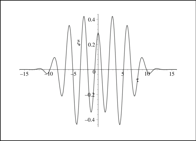
Figure 3: Plot of $\xi(\tau)=R(\tau)-R_{0}$ in the region $-10\leq\tau\leq 10$. The region $\tau<0$ is dominated by the incoming pulse, while that for $\tau>0$ is dominated by the outgoing pulse, resulting from the rebound of the pulse on the symmetry axis. The shell is essentially in its equilibrium radius $R_{0}$ for either $\tau<<-15$ and $\tau>>15$.

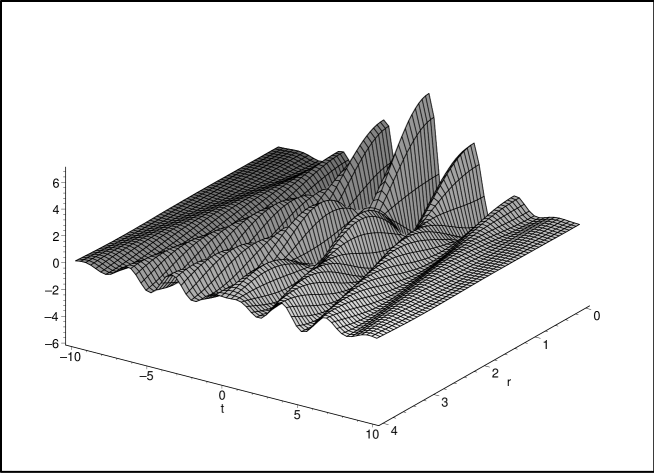
Figure 4: Plot of $\psi_{-}(t,r)$ in the region $0\leq r\leq R_{0}=4$, $-10\leq t\leq 10$. We notice the propagation of the incoming pulse, an intermediate interference zone, formed by incoming and outgoing waves, and the eventual fall off of the pulse as it propagates outside.

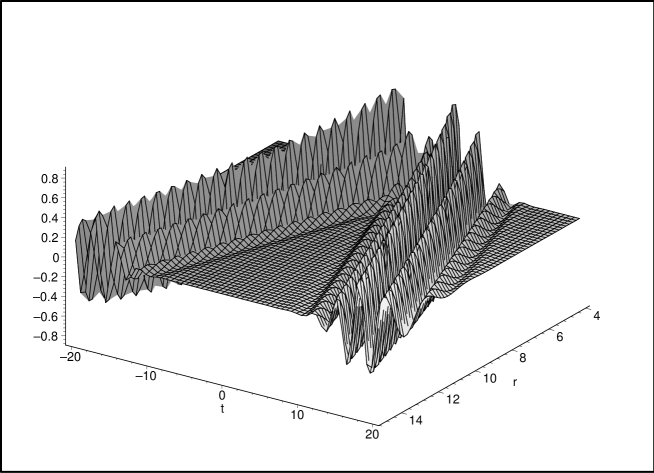
Figure 5: Plot of $\psi_{+}(t,r)$ in the region $4\leq r\leq 15$, $-20\leq t\leq 20$. We can see the propagation of the incoming pulse towards the shell, a zone near $t=0$ where most of the pulse has gone through the shell, and the rebound and propagation of the pulse away from the shell, for $t>0$.

In closing this Section we may ask what is the relation of this construction, and its implied initial data, to the “momentarily static and radiation free” initial data of apostol . (See also nakao for a different analysis of the meaning of this type of data). To understand this we consider again the general equations. Without loss of generality we may choose $\tau$, $t_{-}$, and $t_{+}$ such that $\tau=0$ corresponds to $t_{+}=t_{-}=0$, and then, for the “momentarily static and radiation free” initial data on the surfaces $t_{+}=t_{-}=\tau=0$, we would have,

$$R(\tau) = R_{1}+R_{2}\;\tau^{2}/2+\dots$$

$$\psi_{-}(t_{-},r) = P_{1}(r)\;t_{-}^{2}+\dots$$

$$\gamma_{-}(t_{-},r) = G_{1}(r)\;t_{-}^{2}+\dots$$ (71)

$$\psi_{+}(t_{+},r) = Q_{1}\ln(r/R_{1})+P_{2}(r)\;t_{+}^{2}+\dots$$

$$\gamma_{+}(t_{+},r) = Q_{1}^{2}\ln(r/R_{1})+Q_{2}+G_{2}(r)\;t_{+}^{2}+\dots$$

where $P_{1}$, $P_{2}$, $G_{1}$, and $G_{2}$ are some functions of $r$ that are determined by the evolution, and whose explicit form is not relevant, and dots indicate higher order (in $\tau$ and $t_{\pm}$) terms. Replacing these expressions in the general equations of motion we find that we must set,

$$Q_{{1}} = {\frac{2\lambda\,{R_{{1}}}^{2}}{4\,\lambda\,\left({R_{{1}}}^{2}+{J}^{2}\right)-R_{{1}}\sqrt{{R_{{1}}}^{2}+{J}^{2}}}}$$

$$Q_{{2}} = -\ln\left({\frac{R_{{1}}-4\,\lambda\,\sqrt{{R_{{1}}}^{2}+{J}^{2}}}{R_{{1}}}}\right)$$ (72)

$$R_{{2}} = -{\frac{\left(2\,{J}^{2}+{R_{{1}}}^{2}\right)^{2}\lambda-{J}^{2}\sqrt{{R_{{1}}}^{2}+{J}^{2}}R_{{1}}}{\left({R_{{1}}}^{2}+{J}^{2}\right)^{3/2}{R_{{1}}}^{2}}}$$

We recall now that for a static solution we have,

$$\lambda={\frac{{J}^{2}\sqrt{{R_{{0}}}^{2}+{J}^{2}}R_{{0}}}{\left(2\,{J}^{2}+{R_{{0}}}^{2}\right)^{2}}}$$ (73)

where $R_{0}$ is the equilibrium radius. For small departures from this radius we may set,

$$R_{1}=R_{0}+\xi$$ (74)

where $\xi$ is constant. Replacing (73) and (74) in (VIII), and expanding to first order in $\xi$ we find,

$$Q_{{1}} = -2\,{\frac{{J}^{2}}{{R_{{0}}}^{2}}}+2\,{\frac{{J}^{4}\left(-{R_{{0}}}^{4}+4\,{J}^{2}{R_{{0}}}^{2}+4\,{J}^{4}\right)}{{R_{{0}}}^{7}\left({R_{{0}}}^{2}+{J}^{2}\right)}}\xi+O\left({\xi}^{2}\right)$$

$$Q_{{2}} = -4\,\ln\left(R_{{0}}\right)+2\,\ln\left(2\,{J}^{2}+{R_{{0}}}^{2}\right)-4\,{\frac{{J}^{4}}{{R_{{0}}}^{5}}}\xi+O\left({\xi}^{2}\right)$$ (75)

$$R_{{2}} = {\frac{{J}^{2}\left(-2\,{R_{{0}}}^{4}+{J}^{2}{R_{{0}}}^{2}+2\,{J}^{4}\right)}{\left(2\,{J}^{2}+{R_{{0}}}^{2}\right)\left({R_{{0}}}^{2}+{J}^{2}\right)^{2}{R_{{0}}}^{2}}}\xi+O\left({\xi}^{2}\right)$$

Thus, for sufficiently small departures from the static stable solution the “momentarily static and radiation free” initial data corresponds to adding a constant to $\psi_{+}(0,r)$, while leaving $\psi_{-}(0,r)=0$. As indicated already, it appears possible, at least in principle, to find coefficients in (VIII) that correspond to this initial data, and that could be used to study its evolution, but this problem has not yet been solved. As a final comment, we notice that this does not correspond to perturbations of essentially compact support, and therefore, one would expect that the corresponding integrals would contain some singular expression. This may not be a problem, because to analyze the motion for finite times near this initial data we may simply cut off the perturbation for large $r$, which, from causality, would not modify the solution for times of the order of $r$. We, nevertheless, refer to nakao for a different analysis of this problem.

IX Comments

In this paper we have presented an analysis of the dynamics of a self gravitating cylindrical thin shell of counter rotating dust particles. This analysis provides several new and to a certain extent unexpected results. In particular we show that there exists a family of solutions where the interior of the shell remains flat at all times. For this family the equation of motion for the radius of the shell decouples from the radiative modes. We find a first integral for this equation and show it to be equivalent to that of a particle in a one dimensional time independent potential for a certain value of its total energy. Depending on the constants of the motion we have collapsing, periodic or unbounded solutions. We further analyze under what conditions these solutions are consistent with the field equations for the gravitational modes, and show that there are consistent periodic solutions for the full system. We consider next the dynamics of the system close to a stable static solution in the linearized approximation, where we assume that the interior is regular. The first unexpected result is that we have non trivial solutions for any possible frequency, and that all these modes are stable. The only role played by the Newtonian frequency (corresponding to Newtonian dynamics of the shell) is that it is the only frequency for which the interior is flat. We thus reach the conclusion that the system has no “natural” oscillating frequency that would be slightly modified by the coupling to the radiative modes, but, rather, we have a system where this coupling is “as strong as it can be”, fully determining the behaviour of the shell. We find also an infinite family of “anti-resonances”, where the physical radius of the shell is constant (to first order).

The fact that we have an infinite set of modes suggests that these modes could be used to solve the initial value problem (in the linearized approximation). In fact, we can formally write an arbitrary solution of the field equations as an integral transform involving Bessel functions. Unfortunately, we have not found a way to invert this transforms in such a way that they can be written in terms of arbitrary initial data, although this seems to be possible in principle. We discussed the reasons that make this problem special, and provided a particular example to illustrate some features of the general solution.

References

- (1) T. A. Apostolatos, and K. S. Thorne, Phys. Rev. D 46, 2435 (1992)
- (2) It was assumed in apostol that the MSRF data would always evolve towards a static equilibrium configuration, something that it is not always true, as shown in nakao
- (3) S. M. C. V. Goncalves, Phys. Rev. D, 65, 084045 (2002)
- (4) A. Wang, Phys. Rev. D 72, 108501 (2005)
- (5) P. R. C. T. Pereira, and A. Wang, Phys. Rev. D 62, 124001 (2000), Phys. Rev. D 67, 129902(E) (2003).
- (6) R. J. Gleiser, Phys. Rev. D 65, 068501 (2002).
- (7) M. Seriu, Phys. Rev. D 69, 124030 (2004)
- (8) V. H. Hamity, M. A. Cécere, and D. E. Barraco, Gen. Relativ. Gravit. 41, 2657 (2009)
- (9) A. Einstein, N. Rosen, J. Franklin Inst.223, 43 (1937)
- (10) We are grateful to O. Reula for discussions on this point.
- (11) M. A. Ramirez and R. J. Gleiser, in preparation.
- (12) K. I. Nakao, D. Ida, and Y. Kurita, Phys. Rev. D 77, 044021 (2008)