Accuracy of Transfer Matrix Approaches for Solving the Effective Mass Schrödinger Equation

Abstract

The accuracy of different transfer matrix approaches, widely used to solve the stationary effective mass Schrödinger equation for arbitrary one-dimensional potentials, is investigated analytically and numerically. Both the case of a constant and a position dependent effective mass are considered. Comparisons with a finite difference method are also performed. Based on analytical model potentials as well as self-consistent Schrödinger-Poisson simulations of a heterostructure device, it is shown that a symmetrized transfer matrix approach yields a similar accuracy as the Airy function method at a significantly reduced numerical cost, moreover avoiding the numerical problems associated with Airy functions.

I Introduction

Transfer matrix methods provide an important tool for investigating bound and scattering states in quantum structures. They are mainly used to solve the one-dimensional Schrödinger or effective mass equation, e.g., to obtain the quantized eigenenergies in quantum well heterostructures and metal-oxide-semiconductor structures or the transmission coefficient of potential barriers [1, 2, 3, 4]. Analytical expressions for the transfer matrices are only available in certain cases, as for constant or linear potential sections and potential steps [4]. An arbitrary potential can then be treated by approximating it for example in terms of piecewise constant or linear segments, for which analytical transfer matrices exist. For constant potential segments, the matrices are based on complex exponentials [1, 2], while the linear potential approximation requires the evaluation of Airy functions [2].

Many applications call for highly accurate methods, e.g., quantum cascade laser structures where layer thickness changes by a few Å already lead to significantly modified wavefunctions, resulting in altered device properties [5, 6]. Also numerical efficiency is crucial, especially in cases where the Schrödinger equation has to be solved repeatedly. Examples are the shooting method where the eigenenergies of bound states are found by energy scans, or Schrödinger-Poisson solvers working in an iterative manner [3]. Besides providing accurate results at moderate computational cost, an algorithm is expected to be numerically robust, and a straightforward implementation is also advantageous.

Besides transfer matrices, also other methods are frequently used, in particular finite difference or finite element schemes [7, 8]. For scattering state calculations, they are complimented by suitable transparent boundary conditions, resulting in the Quantum Transmitting Boundary Method (QTBM) [7, 9]. The transfer matrix method tends to be less numerically stable than the QTBM, since for multiple or extended barriers, numerical instabilities can arise due to an exponential blowup caused by roundoff errors [7]. This issue can however be overcome, for example by using a somewhat modified matrix approach, the scattering matrix method [10]. In this case, the transfer matrices of the individual segments are not used to compute the overall transfer matrix, but rather the scattering matrix of the structure. In addition, transfer matrices have many practical properties, such as their intuitiveness particularly for scattering states, the intrinsic current conservation, and the exact treatment of potential steps, which arise at the interfaces of differing materials. This makes them especially suitable and popular for 1-D heterostructures or metal-oxide-semiconductor structures, providing a simple, accurate and efficient simulation method [2].

As mentioned above, transfer matrices are usually based on a piecewise constant or piecewise linear approximation of an arbitrary potential, giving rise to exponential and Airy function solutions, respectively. The main strength of the Airy function approach is that it provides an exact solution for structures consisting of piecewise linear potentials, and hence only requires few segments for approximating almost linear potentials with sufficient accuracy. On the other hand, Airy functions are much more computationally demanding than exponentials, and also prone to numerical overflow for regions with nearly flat potential [11]. Thus, great care has to be taken to avoid these problems, and to evaluate the Airy functions in an efficient way [12].

It would be desirable to combine the advantages of both methods, namely the accuracy of the piecewise linear approximation and the computational convenience of the exponential transfer matrix scheme. In this paper, we evaluate the accuracy and efficiency of the different transfer matrix approaches, taking into account both bound and scattering states. In this context, analytical expressions for the corresponding local discretization error are derived. We furthermore evaluate the different approaches numerically on the basis of an analytically solvable model potential, and also draw comparisons to the QTBM. In particular, we demonstrate that a symmetrized exponential matrix approach is able to provide an accuracy comparable to that of the Airy function method, without having its problems and drawbacks. In our investigation, we will consider both the case of a constant effective mass and the more general case of a position dependent effective mass.

II Transfer matrix approach

In a single-band approximation, the wavefunction $\psi$ of an electron with energy $E$ in a one-dimensional quantum structure can be described by the effective mass equation

$$\left[-\frac{\hbar^{2}}{2}\partial_{z}\frac{1}{m^{\ast}\left(z\right)}\partial_{z}+V(z)-E\right]\psi(z)=0.$$ (1)

Here, the effective mass $m^{\ast}$ and the potential $V$ generally depend on the position $z$ in the structure. For applying the transfer matrix scheme, we divide the structure into segments, see Fig. 1, which can vary in length. Potential and effective mass discontinuities can be treated exactly in transfer matrix approaches by applying corresponding matching conditions. To take advantage of this fact and obtain optimum accuracy, the segments should be chosen so that band edge discontinuities, as introduced by heterostructure interfaces, do not lie within a segment, but rather at the border between two segments.

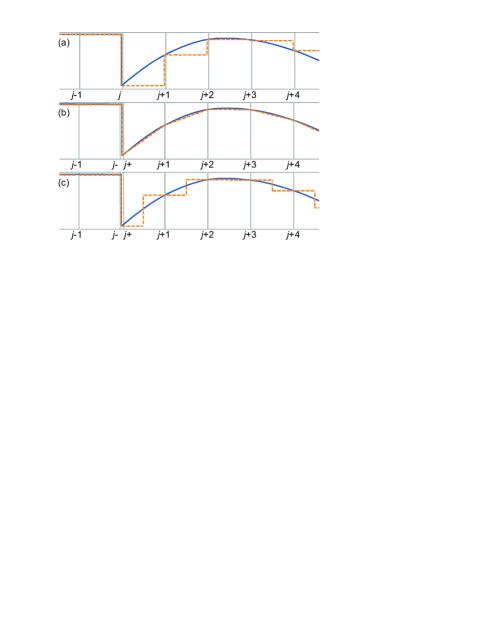
Figure 1: Various transfer matrix schemes applied to segmented potential. Shown is the exact (solid line) and approximated (dashed line) potential. (a) Piecewise constant potential approximation. (b) Piecewise linear approximation. (c) Piecewise contant approximation for symmetrized transfer matrix.

II-A Conventional transfer matrices

For the piecewise constant potential approach (Fig. 1(a)), the potential and effective mass in each segment $j$ are approximated by constant values, e.g., $V_{j}=V\left(z_{j}\right)$, $m_{j}^{\ast}=m^{\ast}\left(z_{j}\right)$ for $z_{j}\leq z<z_{j}+\Delta_{j}=z_{j+1}$, and a jump $V_{j}\rightarrow V_{j+1}$, $m_{j}^{\ast}\rightarrow m_{j+1}^{\ast}$ at the end of the segment [2]. The solution of (1) is for $z_{j}\leq z<z_{j+1}$ then given by

$$\psi\left(z\right)=A_{j}\exp\left[\mathrm{i}k_{j}\left(z-z_{j}\right)\right]+B_{j}\exp\left[-\mathrm{i}k_{j}\left(z-z_{j}\right)\right],$$ (2)

where $k_{j}=\sqrt{2m_{j}^{\ast}\left(E-V_{j}\right)}/\hbar$ is the wavenumber (for $E<V_{j}$, we obtain $k_{j}=\mathrm{i}\kappa_{j}=\mathrm{i}\sqrt{2m_{j}^{\ast}\left(V_{j}-E\right)}/\hbar$) [2]. The matching conditions for the wavefunction at the potential step read

$$\psi\left(z_{0}+\right) =\psi\left(z_{0}-\right),$$

$$\left[\partial_{z}\psi\left(z_{0}+\right)\right]/m^{\ast}\left(z_{0}+\right) =\left[\partial_{z}\psi\left(z_{0}-\right)\right]/m^{\ast}\left(z_{0}-\right),$$ (3)

where $z_{0}+$ and $z_{0}-$ denote the positions directly to the right and left of the step, here located at $z_{0}=z_{j+1}$ [4]. The amplitudes $A_{j+1}$ and $B_{j+1}$ are related to $A_{j}$ and $B_{j}$ by

$$\left(\begin{array}[c]{c}A_{j+1}\\ B_{j+1}\end{array}\right)=T_{j,j+1}\left(\begin{array}[c]{c}A_{j}\\ B_{j}\end{array}\right),$$ (4)

with the transfer matrix

$$T_{j,j+1} =T_{j\rightarrow j+1}T_{j}\left(\Delta_{j}\right)$$

$$=\left(\begin{array}[c]{cc}\frac{\beta_{j+1}+\beta_{j}}{2\beta_{j+1}}e^{\mathrm{i}k_{j}\Delta_{j}}&\frac{\beta_{j+1}-\beta_{j}}{2\beta_{j+1}}e^{-\mathrm{i}k_{j}\Delta_{j}}\\ \frac{\beta_{j+1}-\beta_{j}}{2\beta_{j+1}}e^{\mathrm{i}k_{j}\Delta_{j}}&\frac{\beta_{j+1}+\beta_{j}}{2\beta_{j+1}}e^{-\mathrm{i}k_{j}\Delta_{j}}\end{array}\right).$$ (7)

Equation (7) is the product of the transfer matrix for a flat potential

$$T_{j}\left(\Delta_{j}\right)=\left(\begin{array}[c]{cc}e^{\mathrm{i}k_{j}\Delta_{j}}&0\\ 0&e^{-\mathrm{i}k_{j}\Delta_{j}}\end{array}\right),$$ (8)

obtained from (2), and the potential step matrix

$$T_{j\rightarrow j+1}=\frac{1}{2\beta_{j+1}}\left(\begin{array}[c]{cc}\beta_{j+1}+\beta_{j}&\beta_{j+1}-\beta_{j}\\ \beta_{j+1}-\beta_{j}&\beta_{j+1}+\beta_{j}\end{array}\right)$$ (9)

with $\beta_{j}=k_{j}/m_{j}^{\ast}$, derived from (3) [4]. The relation between the amplitudes at the left and right boundaries of the structure, $A_{0},B_{0}$ and $A_{N},B_{N}$, can be obtained from

$$\left(\begin{array}[c]{c}A_{N}\\ B_{N}\end{array}\right) =T_{N-1,N}T_{N-2,N-1}\dots T_{0,1}\left(\begin{array}[c]{c}A_{0}\\ B_{0}\end{array}\right)$$ (14)

$$=\left(\begin{array}[c]{cc}T_{11}&T_{12}\\ T_{21}&T_{22}\end{array}\right)\left(\begin{array}[c]{c}A_{0}\\ B_{0}\end{array}\right),$$ (19)

where $N$ is the total number of segments. For bound states, this equation must be complemented by suitable boundary conditions. One possibility is to enforce decaying solutions at the boundaries, $A_{0}=B_{N}=0$, corresponding to $T_{22}=0$ in (19), which is satisfied only for specific energies $E$, the eigenenergies of the bound states [2].

For the piecewise linear potential approach (Fig. 1(b)), the potential in each segment $j$ is linearly interpolated, $V\left(z\right)=V_{j}+V_{z,j}\left(z-z_{j}\right)$ for $z_{j}\leq z\leq z_{j}+\Delta_{j}=z_{j+1}$, with $V_{z,j}=\left(V_{j+1}-V_{j}\right)/\Delta_{j}$. Equation (1) can then be solved analytically in terms of the Airy functions $\mathrm{Ai}$ and $\mathrm{Bi}$ [2],

$$\psi\left(z\right)=\mathcal{A}_{j}\mathrm{Ai}\left(s_{j}+\frac{z-z_{j}}{\ell_{j}}\right)+\mathcal{B}_{j}\mathrm{Bi}\left(s_{j}+\frac{z-z_{j}}{\ell_{j}}\right)$$ (20)

for $z_{j}\leq z\leq z_{j+1}$, with $s_{j}=\left(V_{j}-E\right)/\varepsilon_{j}$ and $\ell_{j}=\varepsilon_{j}/V_{z,j}$, where $\varepsilon_{j}=\sqrt[3]{\hbar^{2}V_{z,j}^{2}/\left(2m_{j}^{\ast}\right)}$. We obtain

$$\psi_{j+1} =\mathcal{A}_{j}\mathrm{Ai}(s_{j}+\frac{\Delta_{j}}{\ell_{j}})+\mathcal{B}_{j}\mathrm{Bi}(s_{j}+\frac{\Delta_{j}}{\ell_{j}}),$$

$$\psi_{j+1}^{\prime} =\ell_{j}^{-1}\mathcal{A}_{j}\mathrm{Ai}^{\prime}(s_{j}+\frac{\Delta_{j}}{\ell_{j}})+\ell_{j}^{-1}\mathcal{B}_{j}\mathrm{Bi}^{\prime}(s_{j}+\frac{\Delta_{j}}{\ell_{j}}),$$ (21)

and

$$\mathcal{A}_{j} =D_{j}^{-1}\mathrm{Bi}^{\prime}(s_{j})\psi_{j}-D_{j}^{-1}\ell_{j}\mathrm{Bi}(s_{j})\psi_{j}^{\prime},$$

$$\mathcal{B}_{j} =-D_{j}^{-1}\mathrm{Ai}^{\prime}(s_{j})\psi_{j}+D_{j}^{-1}\ell_{j}\mathrm{Ai}(s_{j})\psi_{j}^{\prime},$$ (22)

with $D_{j}=\mathrm{Ai}(s_{j})\mathrm{Bi}^{\prime}(s_{j})-\mathrm{Ai}^{\prime}(s_{j})\mathrm{Bi}(s_{j})$. Here a prime denotes a derivative with respect to the argument of the Airy function (for $\mathrm{Ai}^{\prime}$, $\mathrm{Bi}^{\prime}$) or the position $z$ (in all other cases). A position dependent effective mass is treated by assigning a constant value to each segment $j$, for example $m^{\ast}\left(z_{j}\right)$ or preferably $\left[m^{\ast}\left(z_{j}\right)+m^{\ast}\left(z_{j+1}\right)\right]/2$ (see appendix), and using the matching conditions (3) at the boundary between two adjacent segments [2]. A piecewise linear interpolation of $m^{\ast}$ as for the potential is not feasible, since then the solutions of (1) cannot be expressed in terms of Airy functions anymore. Equations (21), (22) can again be rewritten as a matrix equation of the form (4), allowing us to treat the quantum structure using (19) in a similar manner as described above [2]. Interfaces introducing abrupt potential changes in the quantum structure must be taken into account explicitly in the Airy function approach by employing the matching conditions (3).

II-B Symmetrized matrix

In the transfer matrix approach, the amplitudes $A_{N}$ and $B_{N}$ at the right boundary of the structure are related to the values $A_{0}$ and $B_{0}$ at the left boundary by repeatedly applying the transfer matrix. Due to the segmentation of the potential, an error is introduced in (19) for every propagation step from a position $z_{j}$ to $z_{j+1}$, which is typically characterized in terms of the local discretization error (LDE). The LDE is defined as the difference between the exact and computed solution at a position $z_{j+1}$ obtained from a given function value at $z_{j}$. In the appendix, the LDE with respect to the amplitudes $A_{j}$ and $B_{j}$ for the transfer matrix (7) is found to be $\mathcal{O}\left(\Delta_{j}^{2}\right)$. It can be improved to $\mathcal{O}\left(\Delta_{j}^{3}\right)$ by symmetrizing the matrix, i.e., placing the potential step in the middle of the segment, see Fig. 1(c). The resulting transfer matrix is then with $k_{j}^{\pm}=\left(k_{j}\pm k_{j+1}\right)/2$ given by

$$T_{j,j+1} =T_{j+1}\left(\frac{\Delta_{j}}{2}\right)T_{j\rightarrow j+1}T_{j}\left(\frac{\Delta_{j}}{2}\right)$$

$$=\left(\begin{array}[c]{cc}\frac{\beta_{j+1}+\beta_{j}}{2\beta_{j+1}}e^{\mathrm{i}k_{j}^{+}\Delta_{j}}&\frac{\beta_{j+1}-\beta_{j}}{2\beta_{j+1}}e^{-\mathrm{i}k_{j}^{-}\Delta_{j}}\\ \frac{\beta_{j+1}-\beta_{j}}{2\beta_{j+1}}e^{\mathrm{i}k_{j}^{-}\Delta_{j}}&\frac{\beta_{j+1}+\beta_{j}}{2\beta_{j+1}}e^{-\mathrm{i}k_{j}^{+}\Delta_{j}}\end{array}\right),$$ (25)

where again $k_{j}=\sqrt{2m_{j}^{\ast}\left(E-V_{j}\right)}/\hbar$, $\beta_{j}=k_{j}/m_{j}^{\ast}$. As in the Airy function approach, interfaces introducing abrupt potential changes in the quantum structure must be dealt with separately by applying the matching conditions; here, the corresponding transfer matrix (9) can be used.

III Comparison

The improved transfer matrix (25) can be evaluated at a comparable computational cost as the matrix (7), but exhibits a superior accuracy. As shown in the appendix, the local discretization error with respect to the amplitudes $A_{j}$ and $B_{j}$ is improved from $\mathcal{O}\left(\Delta_{j}^{2}\right)$ to $\mathcal{O}\left(\Delta_{j}^{3}\right)$ for arbitrary potentials and effective masses, i.e., the same order as for the Airy function approach, which however involves a significantly higher computational effort.

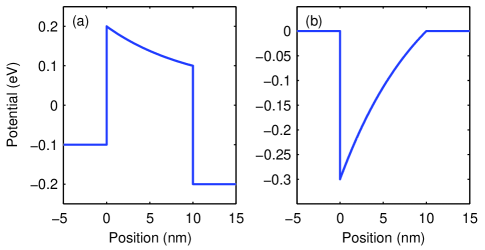
Figure 2: Exponential model potential with $d=10\,\mathrm{nm}$ and $K=-1/d$, used for evaluating the accuracy of various methods. (a) Barrier. (b) Quantum well.

In the following, we compare the accuracy of the different methods for an analytically solvable model potential. Here, polynomial test potentials are not suitable for a general discussion since their higher order derivatives identically vanish, which can lead to an increased accuracy in such special cases. Especially triangular or other piecewise linear potentials are obviously inadequate since the Airy function approach then becomes exact. Instead, we choose the exponential ansatz

$$V(z)=V_{0}+V_{1}\exp\left(Kz\right),$$ (26)

$0\leq z\leq d$ (see Fig. 2), approaching a linear function for $K\rightarrow 0$. Such a potential can for example serve as a model for the effective potential profile in the presence of space charges [13, 14].

III-A Position independent effective mass

For now, we assume a constant effective mass $m^{\ast}$. Then, analytical solutions of the form

$$\psi=c_{1}\mathrm{J}_{\mu}\left(a\right)+c_{2}\mathrm{Y}_{\mu}\left(a\right)$$ (27)

exist for the potential (26), with constants $c_{1}$ and $c_{2}$. Here, $\mathrm{J}_{\mu}$ and $\mathrm{Y}_{\mu}$ are Bessel functions of the first and second kind, and the parameters are given by

$$\mu =2\frac{\sqrt{2m^{\ast}\left(V_{0}-E\right)}}{\hbar K},$$

$$a(z) =2\frac{\sqrt{-2m^{\ast}V_{1}}}{\hbar K}\exp\left(\frac{1}{2}Kz\right).$$ (28)

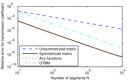
Figure 3: Relative error $\varepsilon_{T}=\left|1-T_{\mathrm{num}}/T\right|$ of the numerically obtained transmission coefficient $T_{\mathrm{num}}$ as a function of the number of segments $N$. The corresponding barrier is shown in Fig. 2(a), the effective mass is assumed to be constant.

For our simulations, the different transfer matrix approaches discussed in Section II are used to compute an overall matrix based on (19), from which the required quantities can be extracted. First, we investigate the barrier structure shown in Fig. 2(a), which can be characterized in terms of a transmission coefficient $T$, giving the tunneling probability of an electron [4]. The unsymmetrized, symmetrized and Airy function transfer matrix approaches are evaluated, based on the expressions (7), (25) and (21), respectively; for comparison, also the QTBM result is computed. Assuming an electron energy of $E=0$ and a constant effective mass of $m^{\ast}=0.067\,m_{e}$ corresponding to GaAs, where $m_{e}$ is the electron mass, the exact value obtained by evaluating (27) is $T=1.749\times 10^{-4}$. Fig. 3 shows the relative error $\varepsilon_{T}\left(N\right)=\left|1-T_{\mathrm{num}}\left(N\right)/T\right|$ as a function of $N\propto\Delta^{-1}$. Here, $T_{\mathrm{num}}\left(N\right)$ is the numerical result for the transmission coefficient, as obtained by the different methods for a subdivision of the structure into $N$ segments of equal length $\Delta=d/N\propto N^{-1}$. As can be seen from Fig. 3, the error scales with $N^{-1}\propto\Delta$ for the unsymmetrized transfer matrix approach and with $N^{-2}\propto\Delta^{2}$ for the other methods. This can easily be understood by means of the local discretization error, which is $\mathcal{O}\left(\Delta^{3}\right)$ for the Airy function approach and the symmetrized transfer matrix, and $\mathcal{O}\left(\Delta^{2}\right)$ for the unsymmetrized matrix, as discussed above and in the appendix. When the overall transfer matrix of the structure is computed from (19), the individual LDEs arising for each of the $N$ segments accumulate, thus resulting in a total error $N\mathcal{O}\left(\Delta^{2}\right)=\mathcal{O}\left(\Delta\right)$ for the unsymmetrized approach and $N\mathcal{O}\left(\Delta^{3}\right)=\mathcal{O}\left(\Delta^{2}\right)$ for the other schemes.

The symmetrized transfer matrix approach and the Airy function method are the most accurate, both exhibiting a comparable error $\varepsilon_{T}\left(N\right)$. However, the symmetrized matrix approach is much more computationally efficient, being over $20$ times faster than the Airy function method in our MATLAB implementation. For a given $N$, the QTBM is even three times faster than the symmetrized matrix approach, but also 40 times less accurate, meaning that it requires $\sqrt{40}\approx 6$ times as many grid points as the symmetrized matrix approach to achieve the same accuracy.

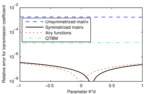
Figure 4: Relative error $\varepsilon_{T}=\left|1-T_{\mathrm{num}}/T\right|$ of the numerically obtained transmission coefficient $T_{\mathrm{num}}$ as a function of $Kd$. Here, $N=1000$ segments are used. The corresponding barrier is shown in Fig. 2(a), the effective mass is assumed to be constant.

Fig. (4) shows again the relative error $\varepsilon_{T}$, but now for a fixed number of segments $N=1000$. Instead, the shape of the potential is modified by varying $K$ in (26), and also adapting $V_{0}$ and $V_{1}$ so that $V\left(z\right)$ remains constant at $z=0$ and $z=d$ and only the curvature of the potential changes. The symmetrized matrix approach and the Airy function method exhibit a superior accuracy especially for small $K$, corresponding to a weak curvature of the potential. While the error of the unsymmetrized matrix approach and the QTBM show only a weak dependence on $K$, the Airy function method becomes exact for $K\rightarrow 0$, where the potential becomes piecewise linear. Interestingly, also the symmetrized transfer matrix approach has a vanishing error $\varepsilon_{T}$ for a specific value of $K$, at $Kd\approx 0.167$.

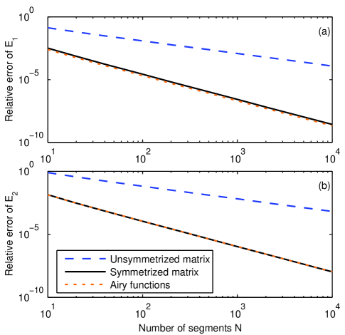
Figure 5: Relative error $\varepsilon_{E}=\left|1-E_{\mathrm{num}}/E\right|$ of the numerically obtained eigenenergy $E_{\mathrm{num}}$ for the (a) first and (b) second bound state as a function of the number of segments $N$. The corresponding well is shown in Fig. 2(b), the effective mass is assumed to be constant.

Now we apply the different numerical methods to the bound states of the potential well shown in Fig. 2(b). Again assuming a constant effective mass of $m^{\ast}=0.067\,m_{e}$, evaluation of (27) yields two bound states with eigenvalues $E_{1}=-0.1343$ $\mathrm{eV}$ and $E_{2}=-0.0129\,\mathrm{eV}$, respectively. In the following, we compare the accuracy of the numerically found eigenenergies $E_{\mathrm{num}}$, as obtained by the unsymmetrized and the symmetrized transfer matrix approach and the Airy function method, corresponding to the expressions (7), (25) and (21), respectively. Here, we again divide the structure into $N$ segments of equal length $\Delta=d/N\propto N^{-1}$. Fig. 5 shows the relative error $\varepsilon_{E}\left(N\right)=\left|1-E_{\mathrm{num}}\left(N\right)/E\right|$ for the first and the second bound state as a function of $N$. As for the transmission coefficient in Fig. 3, the error scales with $N^{-1}\propto\Delta$ for the unsymmetrized matrix approach and with $N^{-2}\propto\Delta^{2}$ for the other methods. Again, the symmetrized matrix approach and the Airy function method exhibit a comparable value of $\varepsilon_{E}\left(N\right)$, being far superior to the unsymmetrized matrix approach.

III-B Position dependent effective mass

Now we compare the accuracy of the different methods for a position dependent effective mass $m^{\ast}(z)$. Here, we choose the same exponential ansatz for the potential as above, see (26) and Fig. 2. For an effective mass of the form $m^{\ast}=m_{0}^{\ast}\exp\left(-Kz\right)$, again an analytical solution exists:

$$\psi=c_{1}\mathrm{J}_{\mu}\left(a\right)\exp\left(-Kz/2\right)+c_{2}\mathrm{Y}_{\mu}\left(a\right)\exp\left(-Kz/2\right),$$ (29)

with

$$\mu =-\sqrt{1+8\frac{m_{0}V_{1}}{K^{2}\hbar^{2}}},$$

$$a(z) =2\frac{\sqrt{-2m_{0}\left(V_{0}-E\right)}}{\hbar K}\exp\left(-\frac{1}{2}Kz\right).$$ (30)

The transfer matrix definitions (7), (25) are also valid for position dependent effective masses. In the Airy function approach (21), a position dependent effective mass can be accounted for by assuming a constant value within each segment, as discussed at the end of Section II-A. Here, we assign the averaged mass $\left(m_{j}^{\ast}+m_{j+1}^{\ast}\right)/2$ rather than $m_{j}^{\ast}$ to each segment, since then the third order LDE, found for the amplitudes $\mathcal{A}$ and $\mathcal{B}$ in the case of position independent masses, is also preserved for the position dependent case, see the appendix.

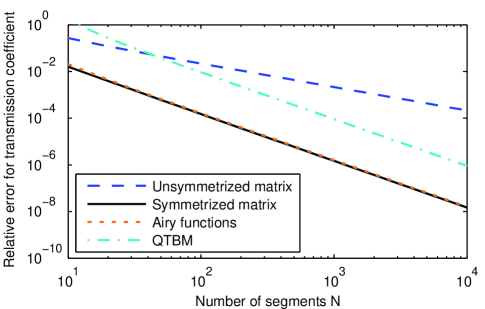
Figure 6: Relative error $\varepsilon_{T}=\left|1-T_{\mathrm{num}}/T\right|$ of the numerically obtained transmission coefficient $T_{\mathrm{num}}$ as a function of the number of segments $N$. The corresponding barrier is shown in Fig. 2(a), the effective mass is assumed to be position dependent.

Fig. 6 corresponds to Fig. 3, but now for a position dependent effective potential with $m^{\ast}=0.2\,m_{e}\exp\left(-Kz\right)$ for $0\leq z\leq d$ and $m^{\ast}=0.067\,m_{e}$ otherwise. The exact transmission coefficient for an electron with energy $E=0$, as obtained by evaluating (29), is now $T=5.376\times 10^{-10}$. From Fig. 6 we can see that also here the error scales with $N^{-1}\propto\Delta$ for the unsymmetrized matrix approach and with $N^{-2}\propto\Delta^{2}$ for the other methods, compare Fig. 3. Again, the symmetrized matrix approach and the Airy function method are the most accurate, with the symmetrized matrix approach being numerically much more efficient.

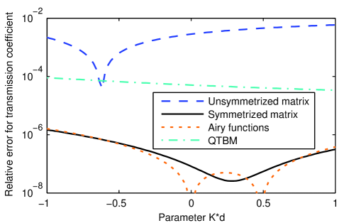
Figure 7: Relative error $\varepsilon_{T}=\left|1-T_{\mathrm{num}}/T\right|$ of the numerically obtained transmission coefficient $T_{\mathrm{num}}$ as a function of $Kd$. Here, $N=1000$ segments are used. The corresponding barrier is shown in Fig. 2(a), the effective mass is assumed to be position dependent.

For the sake of completeness, Fig. (7) is shown as the counterpart of Fig. 4, but now taking into account a position dependent effective mass as above. Again, the symmetrized matrix approach and the Airy function method have a superior accuracy especially for small values of $K$, corresponding to a weak curvature of the potential.

IV Example: Schrödinger-Poisson solver

In the following, we apply the transfer matrices discussed above to a real-world example, namely finding the wavefunctions and eigenenergies of the quantum cascade laser (QCL) structure described in [15]. The goal is to evaluate and compare the performance of the different approaches for a practical problem, and to discuss the inclusion of additional important effects. Specifically, we here also account for energy-band nonparabolicity, and complement the Schrödinger equation by the Poisson equation to take into account space charge effects. In practice, extensive parameter scans have to be performed for QCL design optimization. Thus, the simulation of QCLs calls for especially efficient methods, the more so as the self-consistent solution of the Schrödinger-Poisson system results in a further increase of the numerical effort.

In simulations, the QCL structure is defined by an infinitely repeated elementary sequence of multiple wells and barriers (called a period). For such a structure under bias, it is sufficient to compute the eigenenergies and corresponding wave functions for a single energy interval given by the bias across one period; the solutions of the other periods are then obtained by appropriate shifts in position and energy. We solve the Schrödinger equation using the approaches defined by (7), (25) and (21), respectively. For all three methods, we treat band edge discontinuities at the barrier-well interfaces explicitly using the matching conditions (3), to obtain an optimum accuracy. We use a simulation window of four periods to keep the influence of the boundaries negligible, and determine the bound states similarly as in Section III. To combine reasonable numerical efficiency with a good accuracy, we choose a segment length of $\Delta=2$ $\mathrm{nm}$ (the last segment of each well or barrier is $\Delta\leq 2$ $\mathrm{nm}$).

Various models are available for including nonparabolicity [16]; here, we use an energy dependent effective mass $m_{j}^{\ast}\left(E\right)=m_{j}^{\ast}\left[1+\left(E-V_{j}\right)/E_{g,j}\right]$ (with band gap energy $E_{g,j}$ at position $z_{j}$), which can straightforwardly be implemented into the transfer matrices. The Poisson equation is given by [3, 17]

$$-\partial_{z}\left[\epsilon\left(z\right)\partial_{z}\varphi\left(z\right)\right]=e\left[N\left(z\right)-\sum_{n}n_{\mathrm{2D},n}\left|\psi_{n}\left(z\right)\right|^{2}\right],$$ (31)

leading to an additional potential -e$\varphi$ in (1). Here, $\epsilon\left(z\right)$ is the permittivity, $e$ is the elementary charge, $N\left(z\right)$ is the doping concentration, and $n_{\mathrm{2D},n}$ is the electron sheet density of level $n$ with wave function $\psi_{n}\left(z\right)$. While for an operating QCL, $n_{\mathrm{2D},n}$ can only be exactly determined by detailed carrier transport simulations [6], this is prohibitive for design optimizations of experimental QCL structures over an extended parameter range. Thus, for solving the Schrödinger-Poisson system, simpler and much faster approaches are commonly adopted, such as applying Fermi-Dirac statistics [3, 17]

$$n_{\mathrm{2D},n}=\frac{m^{\ast}}{\pi\hbar^{2}}k_{\mathrm{B}}T\ln\left(1+\exp\left[\left(\mu-\tilde{E}_{n}\right)/\left(k_{\mathrm{B}}T\right)\right]\right),$$ (32)

where $\mu$ is the chemical potential, $k_{\mathrm{B}}$ is the Boltzmann constant, $T$ is the lattice temperature, and $m^{\ast}$ is the effective mass, here taken to be the value of the well material. In (32), we use the energy of a state relative to the conduction band edge $\tilde{E}_{n}=E_{n}-\int V\left|\psi_{n}\right|^{2}\mathrm{d}z$ rather than $E_{n}$ itself to correctly reflect the invariance properties of the biased structure. Especially, this ensures that the simulation results do not depend on the choice of the elementary period in the structure. The chemical potential $\mu$ is found from the charge neutrality condition within one period. The Schrödinger and Poisson equations are iteratively solved until self-consistency is achieved. For the Poisson equation (31), we employ a finite difference scheme on a $1$ Å-grid, where we use (2) and (20) to appropriately interpolate the eigenfunctions obtained from the Schrödinger solver.

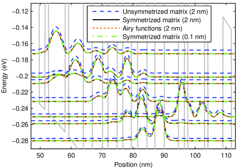
Figure 8: Self-consistent band profile (grey line), energy levels and wave functions squared for the QCL in [15] at a bias of $48$ $\mathrm{kV/cm}$ and a temperature of $300$ $\mathrm{K}$. Shown are the results as obtained with the three transfer matrix methods for $\Delta=2$ $\mathrm{nm}$, and also the symmetrized matrix result for $\Delta=0.1$ $\mathrm{nm}$, which practically coincides with the symmetrized matrix and Airy function results for $\Delta=2$ $\mathrm{nm}$.

Simulations of the QCL in [15] have been performed at various temperatures, considering the seven lowest levels (i.e, with lowest energies $\tilde{E}_{n}$) within each period. In Fig. (8), the obtained energy levels and wave functions squared of a single period are shown for the unsymmetrized, symmetrized and Airy function matrix approach at $T=300$ $\mathrm{K}$, using a segment length of $\Delta=2$ $\mathrm{nm}$. Also the symmetrized transfer matrix result for $\Delta=0.1$ $\mathrm{nm}$ is plotted for reference. The symmetrized matrix and Airy function results exhibit a similar accuracy, with deviations in eigenenergies of around $0.1$ $\mathrm{meV}$ from the high-accuracy result obtained with $\Delta=0.1$ $\mathrm{nm}$. In Fig. (8), those three curves are practically indistinguishable. On the other hand, the unsymmetrized matrix method produces deviations of around $5$ $\mathrm{meV}$. The unsymmetrized and symmetrized matrix approach require approximately the same computation time for obtaining the self-consistent result in Fig. (8), while the Schrödinger-Poisson solver based on the Airy functions is about $10$ times slower. This confirms that the symmetrized transfer matrix method combines high numerical efficiency with excellent accuracy for practical applications.

V Conclusion

In conclusion, we have compared the accuracy of different transfer matrix approaches, as used for solving the effective mass Schrödinger equation with an arbitrary one-dimensional potential and a constant or position dependent effective mass. In particular, the local discretization error has been derived for the Airy function approach resulting from a piecewise linear approximation of the potential, and for unsymmetrized and symmetrized transfer matrices based on a piecewise constant potential approximation. Furthermore, numerical simulations have been performed to evaluate the numerical accuracy of the different approaches for scattering and bound states, employing exponential test potentials. Comparisons to the finite difference method, specifically the QTBM, have also been carried out. Additionally, self-consistent Schrödinger-Poisson device simulations are presented.

The symmetrized transfer matrix approach and the Airy function method exhibit a comparable accuracy, being superior to the other methods investigated. However, the symmetrized matrix approach achieves this at a significantly reduced numerical cost, moreover avoiding the numerical problems associated with Airy functions. All in all, the symmetrized transfer matrix approach is shown to combine the numerical efficiency and straightforwardness of its unsymmetrized counterpart with the superior accuracy of the Airy function method.

Appendix A Local discretization error

In the following, we derive the local discretization error (LDE) for the different types of transfer matrices. In this context, we investigate the piecewise constant potential approximation based on matrix (7) and its symmetrized version (25), as well as the piecewise linear potential scheme (21). As mentioned in Section II, the segments are chosen so that band edge discontinuities in the structure coincide with the borders between two segments, enabling an exact treatment in terms of the matching conditions (3). Thus, for our error analysis we imply that the potential and effective mass vary smoothly within each segment, i.e., have a sufficient degree of differentiability. Otherwise, no further assumptions about the potential shape and effective mass are made. The local discretization error for $\psi$ at $z=z_{j+1}$ is

$$\tau_{j+1}^{\psi}=\psi_{j+1}-\psi\left(z_{j+1}\right),$$ (33)

where $\psi_{j+1}$ is the approximate wavefunction value at $z_{j+1}$ obtained by the transfer matrix approach from a given value $\psi\left(z_{j}\right)=\psi_{j}$ at $z_{j}$, while $\psi\left(z_{j+1}\right)$ is the exact solution. For evaluating the LDE, it is helpful to express $\psi\left(z_{j+1}\right)$ in terms of a Taylor series,

$$\psi\left(z_{j+1}\right) =\psi_{j}+\psi_{j}^{\prime}\Delta_{j}+\frac{1}{2}\psi_{j}^{\prime\prime}\Delta_{j}^{2}+\frac{1}{6}\psi_{j}^{\left(3\right)}\Delta_{j}^{3}$$

$$+\frac{1}{24}\psi_{j}^{\left(4\right)}\Delta_{j}^{4}+\mathcal{O}\left(\Delta_{j}^{5}\right).$$ (34)

Analogously, we can define an LDE for the derivative $\psi^{\prime}$,

$$\tau_{j+1}^{\psi^{\prime}}=\psi_{j+1}^{\prime}-\psi^{\prime}\left(z_{j+1}\right),$$ (35)

and express $\psi^{\prime}\left(z_{j+1}\right)$ as

$$\psi^{\prime}\left(z_{j+1}\right)=\psi_{j}^{\prime}+\psi_{j}^{\prime\prime}\Delta_{j}+\frac{1}{2}\psi_{j}^{\left(3\right)}\Delta_{j}^{2}+\frac{1}{6}\psi_{j}^{\left(4\right)}\Delta_{j}^{3}+\mathcal{O}\left(\Delta_{j}^{4}\right).$$ (36)

A-A Piecewise constant potential approximation

Using (2), we can relate $A_{j}$ and $B_{j}$ to the wavefunction at position $z_{j}$,

$$A_{j} =\frac{1}{2}\left(\psi_{j}-\mathrm{i}\frac{1}{k_{j}}\psi_{j}^{\prime}\right),$$

$$B_{j} =\frac{1}{2}\left(\psi_{j}+\mathrm{i}\frac{1}{k_{j}}\psi_{j}^{\prime}\right),$$ (37)

and express the LDEs for the amplitudes $A$ and $B$ in terms of $\tau_{j+1}^{\psi}$ and $\tau_{j+1}^{\psi^{\prime}}$,

$$\tau_{j+1}^{A} =A_{j+1}-A\left(z_{j+1}\right)=\frac{1}{2}\left(\tau_{j+1}^{\psi}-\mathrm{i}\frac{1}{k_{j+1}}\tau_{j+1}^{\psi^{\prime}}\right),$$

$$\tau_{j+1}^{B} =B_{j+1}-B\left(z_{j+1}\right)=\frac{1}{2}\left(\tau_{j+1}^{\psi}+\mathrm{i}\frac{1}{k_{j+1}}\tau_{j+1}^{\psi^{\prime}}\right).$$ (38)

For the unsymmetrized transfer matrix, we obtain from (2) with the expressions (4) and (7)

$$\psi_{j+1} =A_{j+1}+B_{j+1}=\exp\left(\mathrm{i}k_{j}\Delta_{j}\right)A_{j}+\exp\left(-\mathrm{i}k_{j}\Delta_{j}\right)B_{j},$$

$$\psi_{j+1}^{\prime} =\mathrm{i}k_{j+1}\left(A_{j+1}-B_{j+1}\right)$$

$$=\mathrm{i}k_{j+1}\frac{\beta_{j}}{\beta_{j+1}}\left[A_{j}\exp\left(\mathrm{i}k_{j}\Delta_{j}\right)-B_{j}\exp\left(-\mathrm{i}k_{j}\Delta_{j}\right)\right].$$ (39)

For calculating the LDE, we insert the expressions (39) and (34) into (33), where we express $A_{j}$ and $B_{j}$ by (37) and use (1) to rewrite the derivatives $\psi_{j}^{\left(n\right)}$ in (34) as

$$\psi_{j}^{\prime\prime} =-k_{j}^{2}\psi_{j}+\frac{m_{j}^{\ast\prime}}{m_{j}^{\ast}}\psi_{j}^{\prime},$$

$$\psi_{j}^{\left(3\right)} =-\frac{\left(m_{j}^{\ast}k_{j}^{2}\right)^{\prime}}{m_{j}^{\ast}}\psi_{j}-k_{j}^{2}\psi_{j}^{\prime}+\frac{m_{j}^{\ast\prime\prime}}{m_{j}^{\ast}}\psi_{j}^{\prime},$$ (40)

with $k_{j}=\sqrt{2m_{j}^{\ast}\left(E-V_{j}\right)}/\hbar$. A Taylor expansion then yields

$$\tau_{j+1}^{\psi} =\cos\left(k_{j}\Delta_{j}\right)\psi_{j}+\sin\left(k_{j}\Delta_{j}\right)k_{j}^{-1}\psi_{j}^{\prime}$$

$$-\psi_{j}-\psi_{j}^{\prime}\Delta_{j}-\frac{1}{2}\psi_{j}^{\prime\prime}\Delta_{j}^{2}-\frac{1}{6}\psi_{j}^{\left(3\right)}\Delta_{j}^{3}+\mathcal{O}\left(\Delta_{j}^{4}\right)$$

$$=-\frac{1}{2}\frac{m_{j}^{\ast\prime}}{m_{j}^{\ast}}\psi_{j}^{\prime}\Delta_{j}^{2}+\frac{1}{6}\left(\frac{\left(m_{j}^{\ast}k_{j}^{2}\right)^{\prime}}{m_{j}^{\ast}}\psi_{j}-\frac{m_{j}^{\ast\prime\prime}}{m_{j}^{\ast}}\psi_{j}^{\prime}\right)\Delta_{j}^{3}$$

$$+\mathcal{O}\left(\Delta_{j}^{4}\right).$$ (41)

Analogously, by inserting the expressions (39) and (36) into (35) we obtain

$$\tau_{j+1}^{\psi^{\prime}} =\frac{m_{j+1}^{\ast}}{m_{j}^{\ast}}\left(\psi_{j}^{\prime}\cos\left(k_{j}\Delta_{j}\right)-k_{j}\sin\left(k_{j}\Delta_{j}\right)\psi_{j}\right)$$

$$-\psi_{j}^{\prime}-\psi_{j}^{\prime\prime}\Delta_{j}-\frac{1}{2}\psi_{j}^{\left(3\right)}\Delta_{j}^{2}+\mathcal{O}\left(\Delta_{j}^{3}\right)$$

$$=\left(\frac{m_{j+1}^{\ast}}{m_{j}^{\ast}}-1-\frac{m_{j}^{\ast\prime}}{m_{j}^{\ast}}\Delta_{j}\right)\psi_{j}^{\prime}+\frac{m_{j}^{\ast}-m_{j+1}^{\ast}}{m_{j}^{\ast}}k_{j}^{2}\psi_{j}\Delta_{j}$$

$$+\frac{1}{2}\left(\frac{\left(m_{j}^{\ast}k_{j}^{2}\right)^{\prime}}{m_{j}^{\ast}}\psi_{j}-\frac{m_{j}^{\ast\prime\prime}}{m_{j}^{\ast}}\psi_{j}^{\prime}+\frac{m_{j}^{\ast}-m_{j+1}^{\ast}}{m_{j}^{\ast}}k_{j}^{2}\psi_{j}^{\prime}\right)\Delta_{j}^{2}$$

$$+\mathcal{O}\left(\Delta_{j}^{3}\right)$$

$$=\left(\frac{\left(m_{j}^{\ast}k_{j}^{2}\right)^{\prime}}{2m_{j}^{\ast}}-\frac{m_{j}^{\ast\prime}}{m_{j}^{\ast}}k_{j}^{2}\right)\psi_{j}\Delta_{j}^{2}+\mathcal{O}\left(\Delta_{j}^{3}\right),$$ (42)

where we use $m_{j+1}^{\ast}=m_{j}^{\ast}+m_{j}^{\ast\prime}\Delta_{j}+\frac{1}{2}m_{j}^{\ast\prime\prime}\Delta_{j}^{2}+\mathcal{O}\left(\Delta_{j}^{3}\right)$ to obtain the last line of (42). Thus, $\tau_{j+1}^{\psi}\$is $\mathcal{O}\left(\Delta_{j}^{2}\right)$ ($\mathcal{O}\left(\Delta_{j}^{3}\right)$ for a constant effective mass), and $\tau_{j+1}^{\psi^{\prime}}=\mathcal{O}\left(\Delta_{j}^{2}\right)$. With (38), we see that both $\tau_{j+1}^{A}$ and $\tau_{j+1}^{B}$ are $\mathcal{O}\left(\Delta_{j}^{2}\right)$.

In a similar manner, we obtain for the symmetrized matrix (25) $\tau_{j+1}^{\psi}=\mathcal{O}\left(\Delta_{j}^{3}\right)$ and $\tau_{j+1}^{\psi^{\prime}}=\mathcal{O}\left(\Delta_{j}^{3}\right)$. More precisely, the calculation yields for a constant $m^{\ast}$

$$\tau_{j+1}^{\psi} =\frac{1}{24}\left(k_{j}^{2}\right)^{\prime}\psi_{j}\Delta_{j}^{3}+\mathcal{O}\left(\Delta_{j}^{4}\right),$$

$$\tau_{j+1}^{\psi^{\prime}} =-\frac{1}{12}\left(k_{j}^{2}\right)^{\prime\prime}\psi_{j}\Delta_{j}^{3}-\frac{1}{24}\left(k_{j}^{2}\right)^{\prime}\psi_{j}^{\prime}\Delta_{j}^{3}+\mathcal{O}\left(\Delta_{j}^{4}\right)$$ (43)

(and a somewhat more complicated expression for a position dependent effective mass). This means that $\tau_{j+1}^{A}$ and $\tau_{j+1}^{B}$ are now $\mathcal{O}\left(\Delta_{j}^{3}\right)$.

A-B Piecewise linear potential approximation

For computing the LDEs (33) and (35) of the Airy function approach, we proceed in a manner similar as above. Equations (21) and (22) give the relation between values $\psi_{j}$, $\psi_{j}^{\prime}$ at $z_{j}$ and the numerical result $\psi_{j+1}$, $\psi_{j+1}^{\prime}$ obtained at $z_{j+1}$ from the Airy function approach:

$$\psi_{j+1} =\frac{1}{D_{j}}\left[\mathrm{Ai}(s_{j}+\frac{\Delta_{j}}{\ell_{j}})\mathrm{Bi}^{\prime}(s_{j})-\mathrm{Ai}^{\prime}(s_{j})\mathrm{Bi}(s_{j}+\frac{\Delta_{j}}{\ell_{j}})\right]\psi_{j}$$

$$+\frac{\ell_{j}}{D_{j}}\left[\mathrm{Ai}(s_{j})\mathrm{Bi}(s_{j}+\frac{\Delta_{j}}{\ell_{j}})-\mathrm{Ai}(s_{j}+\frac{\Delta_{j}}{\ell_{j}})\mathrm{Bi}(s_{j})\right]\psi_{j}^{\prime}$$

$$=\left(1+\frac{1}{2}\frac{s_{j}}{\ell_{j}^{2}}\Delta_{j}^{2}+\frac{1}{6}\frac{\Delta_{j}^{3}}{\ell_{j}^{3}}+\frac{1}{24}\frac{s_{j}^{2}}{\ell_{j}^{4}}\Delta_{j}^{4}\right)\psi_{j}$$

$$+\left(\Delta_{j}+\frac{1}{6}\frac{s_{j}}{\ell_{j}^{2}}\Delta_{j}^{3}+\frac{1}{12}\frac{\Delta_{j}^{4}}{\ell_{j}^{3}}\right)\psi_{j}^{\prime}+\mathcal{O}\left(\Delta_{j}^{5}\right),$$ (44)

$$\psi_{j+1}^{\prime} =\frac{1}{D_{j}\ell_{j}}\left[\mathrm{Ai}^{\prime}(s_{j}+\frac{\Delta_{j}}{\ell_{j}})\mathrm{Bi}^{\prime}(s_{j})\right.$$

$$\left.-\mathrm{Bi}^{\prime}(s_{j}+\frac{\Delta_{j}}{\ell_{j}})\mathrm{Ai}^{\prime}(s_{j})\right]\psi_{j}$$

$$+\frac{1}{D_{j}}\left[\mathrm{Ai}(s_{j})\mathrm{Bi}^{\prime}(s_{j}+\frac{\Delta_{j}}{\ell_{j}})-\mathrm{Ai}^{\prime}(s_{j}+\frac{\Delta_{j}}{\ell_{j}})\mathrm{Bi}(s_{j})\right]\psi_{j}^{\prime}$$

$$=\left(s_{j}\frac{\Delta_{j}}{\ell_{j}^{2}}+\frac{1}{2}\frac{1}{\ell_{j}^{3}}\Delta_{j}^{2}+\frac{1}{6}\frac{s_{j}^{2}}{\ell_{j}^{4}}\Delta_{j}^{3}\right)\psi_{j}$$

$$+\left(1+\frac{1}{2}\frac{s_{j}}{\ell_{j}^{2}}\Delta_{j}^{2}+\frac{1}{3}\frac{\Delta_{j}^{3}}{\ell_{j}^{3}}\right)\psi_{j}^{\prime}+\mathcal{O}\left(\Delta_{j}^{4}\right),$$ (45)

with $D_{j}=\mathrm{Ai}(s_{j})\mathrm{Bi}^{\prime}(s_{j})-\mathrm{Ai}^{\prime}(s_{j})\mathrm{Bi}(s_{j})$. The exact results $\psi\left(z_{j+1}\right)$ and $\psi^{\prime}\left(z_{j+1}\right)$ are again expressed by the Taylor series expansions (34) and (36), respectively, where we rewrite the derivatives $\psi_{j}^{\left(n\right)}$ in terms of $\psi_{j}$ and $\psi_{j}^{\prime}$. For a constant effective mass, we have

$$\psi_{j}^{\prime\prime} =\ell_{j}^{-2}s_{j}\psi_{j},$$

$$\psi_{j}^{\left(3\right)} =\ell_{j}^{-2}s_{j}\psi_{j}^{\prime}+\ell_{j}^{-3}\frac{V_{j}^{\prime}}{V_{z,j}}\psi_{j},$$

$$\psi_{j}^{\left(4\right)} =\ell_{j}^{-4}s_{j}^{2}\psi_{j}+2\ell_{j}^{-3}\frac{V_{j}^{\prime}}{V_{z,j}}\psi_{j}^{\prime}+\ell_{j}^{-3}\frac{V_{j}^{\prime\prime}}{V_{z,j}}\psi_{j},$$ (46)

with $V_{z,j}=\left(V_{j+1}-V_{j}\right)/\Delta_{j}$, and obtain with the expressions (33), (34) and (44)

$$\tau_{j+1}^{\psi}=\psi_{j+1}-\psi\left(z_{j+1}\right)=-\frac{1}{24}\left(k_{j}^{2}\right)^{\prime\prime}\psi_{j}\Delta_{j}^{4}+\mathcal{O}\left(\Delta_{j}^{5}\right),$$ (47)

and with (35), (36) and (45)

$$\tau_{j+1}^{\psi^{\prime}}=\psi_{j+1}^{\prime}-\psi^{\prime}\left(z_{j+1}\right)=-\frac{1}{12}\left(k_{j}^{2}\right)^{\prime\prime}\psi_{j}\Delta_{j}^{3}+\mathcal{O}\left(\Delta_{j}^{4}\right),$$ (48)

where $k_{j}=\sqrt{2m_{j}^{\ast}\left(E-V_{j}\right)}/\hbar$. Using (22), we can express the LDEs for the amplitudes $\mathcal{A}$ and $\mathcal{B}$ in terms of $\tau_{j+1}^{\psi}$ and $\tau_{j+1}^{\psi^{\prime}}$, and obtain $\tau_{j+1}^{\mathcal{A}}=\mathcal{O}\left(\Delta_{j}^{3}\right)$, $\tau_{j+1}^{\mathcal{B}}=\mathcal{O}\left(\Delta_{j}^{3}\right)$.

As described in Section II-A, a position dependent effective mass can in the Airy function approach be treated by assuming a constant value within each segment $j$, e.g., $m_{j}^{\ast}=m^{\ast}\left(z_{j}\right)$, and applying the matching conditions (3) at the section boundaries [2]. The result for $\psi_{j+1}^{\prime}$ in (45) has thus to be multiplied by $m_{j+1}^{\ast}/m_{j}^{\ast}$ before inserting it into (35). While $\tau_{j+1}^{\psi^{\prime}}$ is still $\mathcal{O}\left(\Delta_{j}^{3}\right)$, $\tau_{j+1}^{\psi}$ drops to $\mathcal{O}\left(\Delta_{j}^{2}\right)$, now yielding $\tau_{j+1}^{\mathcal{A}}=\mathcal{O}\left(\Delta_{j}^{2}\right)$, $\tau_{j+1}^{\mathcal{B}}=\mathcal{O}\left(\Delta_{j}^{2}\right)$. The error analysis also shows that $\tau_{j+1}^{\psi}$ and thus $\tau_{j+1}^{\mathcal{A}},\tau_{j+1}^{\mathcal{B}}$ can be improved to $\mathcal{O}\left(\Delta_{j}^{3}\right)$ by assigning an averaged mass $\left(m_{j}^{\ast}+m_{j+1}^{\ast}\right)/2$ rather than $m_{j}^{\ast}$ to each segment, and applying the matching conditions correspondingly.

Christian Jirauschek Christian Jirauschek was born in Karlsruhe, Germany, in 1974. He received his Dipl-Ing. and doctoral degrees in electrical engineering in 2000 and 2004, respectively, from the Universität Karlsruhe (TH), Germany. From 2002 to 2005, he was a Visiting Scientist at the Massachusetts Institute of Technology (MIT), Cambridge, MA. Since 2005, he has been with the TU München in Germany, first as a Postdoctoral Fellow and since 2007 as the Head of an Independent Junior Research Group (Emmy-Noether Program of the DFG). His research interests include modeling in the areas of optics and device physics, especially the simulation of quantum devices and mode-locked laser theory. Dr. Jirauschek is a member of the IEEE, the German Physical Society (DPG), and the Optical Society of America. Between 1997 and 2000, he held a scholarship from the German National Merit Foundation (Studienstiftung des Deutschen Volkes).

References

- [1] Y. Ando and T. Itoh, “Calculation of transmission tunneling current across arbitrary potential barriers,” J. Appl. Phys., vol. 61, pp. 1497–1502, Feb. 1987.
- [2] B. Jonsson and S. T. Eng, “Solving the Schrödinger equation in arbitrary quantum-well potential profiles using the transfer matrix method,” IEEE J. Quantum Electron., vol. 26, pp. 2025–2035, 1990.
- [3] E. Cassan, “On the reduction of direct tunneling leakage through ultrathin gate oxides by a one-dimensional Schrödinger-Poisson solver,” J. Appl. Phys., vol. 87, pp. 7931–7939, Jun. 2000.
- [4] J. H. Davies, The Physics of Low-dimensional Semiconductors. Cambridge University Press, Dec. 1997.
- [5] M. S. Vitiello, G. Scamarcio, V. Spagnolo, B. S. Williams, S. Kumar, Q. Hu, and J. L. Reno, “Measurement of subband electronic temperatures and population inversion in THz quantum-cascade lasers,” Appl. Phys. Lett., vol. 86, no. 11, pp. 111 115–1–3, Mar. 2005.
- [6] C. Jirauschek, G. Scarpa, P. Lugli, M. S. Vitiello, and G. Scamarcio, “Comparative analysis of resonant phonon THz quantum cascade lasers,” J. Appl. Phys., vol. 101, no. 8, pp. 086 109–1–3, Apr. 2007.
- [7] W. R. Frensley, “Quantum transport,” in Heterostructures and Quantum Devices, ser. VLSI Electronics: Microstructure Science, W. R. Frensley and N. G. Einspruch, Eds. Academic Press, 1994.
- [8] C. Juang, K. J. Kuhn, and R. B. Darling, “Stark shift and field-induced tunneling in AlxGa1-xAs/GaAs quantum-well structures,” Phys. Rev. B, vol. 41, pp. 12 047–12 053, Jun. 1990.
- [9] C. S. Lent and D. J. Kirkner, “The quantum transmitting boundary method,” J. Appl. Phys., vol. 67, pp. 6353–6359, May 1990.
- [10] D. Y. Ko and J. C. Inkson, “Matrix method for tunneling in heterostructures: Resonant tunneling in multilayer systems,” Phys. Rev. B, vol. 38, pp. 9945–9951, Nov. 1988.
- [11] S. Vatannia and G. Gildenblat, “Airy’s functions implementation of the transfer-matrix method for resonant tunneling in variably spaced finite superlattices.” IEEE J. Quantum Electron., vol. 32, pp. 1093–1105, Jun. 1996.
- [12] J.-G. S. Demers and R. Maciejko, “Propagation matrix formalism and efficient linear potential solution to Schrödinger’s equation,” J. Appl. Phys., vol. 90, pp. 6120–6129, Dec. 2001.
- [13] S. Saito, K. Torii, M. Hiratani, and T. Onai, “Analytical quantum mechanical model for accumulation capacitance of MOS structures,” IEEE Electron Device Lett., vol. 23, pp. 348–350, Jun. 2002.
- [14] E. P. Nakhmedov, C. Radehaus, and K. Wieczorek, “Study of direct tunneling current oscillations in ultrathin gate dielectrics,” J. Appl. Phys., vol. 97, no. 6, pp. 064 107–1–7, Mar. 2005.
- [15] H. Page, C. Becker, A. Robertson, G. Glastre, V. Ortiz, and C. Sirtori, “300 K operation of a GaAs-based quantum-cascade laser at m,” Appl. Phys. Lett., vol. 78, pp. 3529–3531, May 2001.
- [16] D. F. Nelson, R. C. Miller, and D. A. Kleinman, “Band nonparabolicity effects in semiconductor quantum wells,” Phys. Rev. B, vol. 35, pp. 7770–7773, May 1987.
- [17] H. Li, J. C. Cao, and H. C. Liu, “Effects of design parameters on the performance of terahertz quantum-cascade lasers,” Semicond. Sci. Technol., vol. 23, no. 12, pp. 125 040–1–6, Dec. 2008.