Statistical Modeling of RNA-Seq Data

Abstract

Recently, ultra high-throughput sequencing of RNA (RNA-Seq) has been developed as an approach for analysis of gene expression. By obtaining tens or even hundreds of millions of reads of transcribed sequences, an RNA-Seq experiment can offer a comprehensive survey of the population of genes (transcripts) in any sample of interest. This paper introduces a statistical model for estimating isoform abundance from RNA-Seq data and is flexible enough to accommodate both single end and paired end RNA-Seq data and sampling bias along the length of the transcript. Based on the derivation of minimal sufficient statistics for the model, a computationally feasible implementation of the maximum likelihood estimator of the model is provided. Further, it is shown that using paired end RNA-Seq provides more accurate isoform abundance estimates than single end sequencing at fixed sequencing depth. Simulation studies are also given.

, and

t1These authors contributed equally to this work and are both corresponding authors.

1 Introduction

1.1 Biological Background

All cells in an individual mammal have almost identical DNA. Yet, cell function within an organism has huge variation. One mechanism that differentiates cell function is its gene expression pattern. Recent research has shown that this differentiation may be on a fine scale: that subtle sequence variants of expressed genes (also referred to as transcripts), called isoforms, have significant impact on the function of the proteins encoded by the RNA and hence their function in the cell (see, e.g., Wang et al. (2008)). The purpose of this paper is to develop and analyze statistical methodology for measuring differential expression of isoforms using an emerging powerful technology called Ultra High Throughput Sequencing (UHTS). Such study has the potential to help reveal new insights into cellular isoform level gene expression patterns and mechanisms, including characteristics of cell specific specialization.

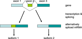
Figure 1: A gene (DNA sequence) with three exons. During transcription, two isoforms are generated. The first isoform contains all of the gene’s three exons. The second isoform contains the first and third exon, skipping the middle exon. This process is called alternative splicing and the middle exon is called an alternatively spliced exon.

The central dogma in biology describes the information transfer that allows cells to generate proteins, the building blocks of biological function. This dogma states that DNA is transcribed to messenger RNA (mRNA) which is in turn translated into proteins. Recent discoveries have highlighted the importance of regulation at the level of mRNA, showing that protein levels and function can be regulated by subtle differences in the sequence of mRNA molecules in a cell.

In bacteria, short DNA sequences are transcribed in a one to one fashion to mRNA. This mRNA is referred to as a gene or a transcript. Like DNA, each mRNA is a string of nucleotides, each position taking four possible values. Mammalian cells commonly generate a large class of mRNA molecules from a single relatively short DNA sequence. The set of such mRNA molecules are called isoforms of a gene. This paper concentrates on one common mechanism generating isoforms called alternative splicing. An example of alternative splicing is depicted in Figure 1: two isoforms can arise from the same gene when the DNA, which is comprised of three sequence blocks (called exons), can be transcribed into two different mRNA molecules: one of which contains all three exons and one of which only contains the first and third exon. As this example shows, isoforms typically have highly similar sequence. Despite this sequence similarity, isoforms can encode proteins which may have different functional roles. Further, most genes have more than three exons, and alternative use of exons can give rise to large numbers of isoforms. Thus, it has been historically difficult for technology and statistical methods to allow researchers to distinguish between different isoforms of the same gene.

1.2 Ultra High Throughput Sequencing

Ultra High Throughput Sequencing (UHTS or simply “sequencing”) is an emerging technology which promises to become as (or more) powerful, popular and cost-effective than current microarray technology for several applications, including isoform estimation. When used to study mRNA levels, UHTS is referred to as RNA-Seq. In the past year, studies using UHTS to study genome organization, including isoform expression, have been prominent (see Pan et al. (2008); Zhang et al. (2009); Wahlstedt et al. (2009); Hansen et al. (2009); Maher et al. (2009)) and featured in the journals Science and Nature (see Sultan et al. (2008); Wang et al. (2008)), which dubbed 2007 as the “year of sequencing” (see Chi (2008)).

Briefly, UHTS is a method that relies on directly sequencing the nucleotides in a sample rather than inferring abundance of mRNA by measuring intensities using predetermined homologous probes as microarrays do. Thus, the data generated from an UHTS experiment are large numbers of discrete strings of nucleotides, called base pairs (bp), which can take values of A, C, G or T. In 2010, each experiment produced tens of millions of up to 100bp reads. The throughput of this technology is expected to continue its rapid growth.

Two experimental protocols for RNA-Seq are in common use: (a) single end and (b) paired end sequencing experiments. For single end experiments, one end (typically about 50–100 bp) of a long (typically 200–400 nucleotide) molecule is sequenced. For paired end experiments, typically 50–100 bp of both ends of a typically 200–400 nucleotide molecule are sequenced. Using current Illumina technology, each time the sequencing machine is operated, eight samples (e.g., potentially eight different catalogues of gene expression) can be interrogated (essentially) independently and tens of millions of reads are produced in each sample.

1.3 Related Work

An important application and use of UHTS technology is to quantify the abundance of mRNA in a cell (RNA-Seq). This is done by matching the sequences generated in an UHTS experiment to a database of known mRNA sequences (called alignment) and inferring the abundance of each mRNA from the number of experimental reads (fragments of the original mRNA molecules) aligning to it. Sometimes, a statistical model is used for this estimate. Importantly, experimental steps involved in an UHTS experiment can affect the probability of each fragment being observed, although modeling of these processes is not the focus of this paper.

The rapid technological advances in sequencing have spawned a large number of algorithms for analyzing sequence data (see Langmead et al. (2009); Trapnell, Pachter and Salzberg (2009); Trapnell et al. (2010); Mortazavi et al. (2008)), some of which aim to estimate mRNA abundance. To date, inference on the abundance of mRNA has been made by aligning reads to known genes and estimating a gene’s expression by averaging the number of reads which map uniquely to it using the simplifying assumption that the transcript is sampled uniformly (see Jiang and Wong (2009); Mortazavi et al. (2008)), and sometimes using heuristic approaches to accommodate reads which map to multiple locations (see Mortazavi et al. (2008)). These models do not provide optimal estimators of isoform-specific expression levels and do not accommodate modeling of important steps in the experimental procedure. The work in this paper significantly extends a basic Poisson model developed in Jiang and Wong (2009) to allow for more flexible and efficient inference and establish rigorous statistical theory. In particular, the model in Jiang and Wong (2009) does not work with paired end sequencing data, or read-specific sample rate in a sequencing protocol.

This paper introduces a statistical model for estimating isoform abundance from RNA-Seq data. By grouping the reads into categories and modeling the read counts within each category as Poisson variables, the model is flexible enough to accommodate both single end and paired end RNA-Seq data. Based on the derivation of minimal sufficient statistics, a computationally feasible implementation of the maximum likelihood estimator of the model is provided. Using a study of the Fisher information and also numerical simulation, it is shown that using paired end RNA-Seq one can get more accurate isoform abundance estimates. To the best of our knowledge, this is the first such statistically rigorous methodology and analysis to be developed.

2 RNA-Seq

Isoforms of a gene are subtle differences in a gene sequence, sometimes resulting from inclusion or exclusion of a single exon, a discrete piece of sequence depicted in Figure 1. In principle, compared to microarrays, UHTS has the potential to provide high resolution estimates of isoform use. However, signal deconvolution must take place for these estimates to be accurate.

In order to estimate the expression of different isoforms of the same gene, several measurements of that gene’s expression, whether from a microarray or sequencing, must be deconvolved. Several studies have investigated this deconvolution problem when measurements are made from a microarray (see Hiller et al. (2009) or She, Hubbell and Wang (2009)). This paper presents an estimator for deconvolution for ultra high throughput sequencing experiments.

As mentioned, two experimental approaches for RNA-Seq are in wide use. In single end read experiments, reads are generated from one end of a molecule (depicted schematically in Figure 2); in paired end reads, reads are generated from both ends of a molecule, but typically a large number of nucleotides interior to the molecule are left unsequenced (depicted schematically in Figure 3). The length of the whole molecule being sequenced is called the insert size or insert length.

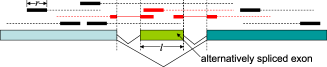
Figure 2: Single end sequencing. A gene of three exons is shown with the middle exon of length $l$ being alternatively spliced. Reads that come from this gene are shown above the gene in solid bars and the parts that are not sequenced are shown in broken lines. Reads that span an exon–exon junction are shown in solid bars connected by thin lines. Reads that are related to the AS exon are shown in red color. In this case only the reads in red are isoform informative.

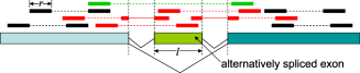
Figure 3: Paired end sequencing. A gene of three exons is shown with the middle exon of length $l$ being alternatively spliced. Paired end reads that come from this gene are shown above the gene in solid bars and the parts that are not sequenced are shown in broken lines. Reads that span an exon–exon junction are shown in solid bars connected by thin line. Reads that are directly related to the AS exon are in red as before. Reads that provide indirect information for separating isoform expressions are in green.

To appreciate the additional information provided by the paired end reads, consider Figure 2 which depicts single end reads randomly sampled from a transcript of a gene. Suppose there are two possible isoforms for the transcript of this gene depending on whether an exon of length $l$ is retained or skipped. In this case, only the reads that come from the alternatively spliced exon (AS exon), or come from junctions involving either the AS exon or the two neighboring exons, can provide information to distinguish the two isoforms from each other, that is, only these reads are isoform informative. If the AS exon is short compared to the transcript, then the majority of the single end reads contain information only on gene level expression but not isoform level expression. Assuming uniform distribution on the reads’ positions in the gene, it is evident that a read is related to the AS exon with probability $P={\frac{l+r}{L-r}}$ if the read comes from the AS exon inclusive isoform, where $L$ is the length of the whole gene (without the intronic regions) and $r$ is the length of the reads. Thus, $P$ is a strictly increasing function with respect to the read length $r$ as well as the AS exon length $l$. As an example, for a gene of length 2000 bp with a short AS exon of length 50 bp, $P=0.0406$ for reads of length 30 bp, $P=0.0513$ for reads of length 50 bp, and $P=0.0789$ for reads of length 100 bp.

Currently, technical limitations limit the length of sequenced reads. These limitations vary by particular platform used for UHTS. The two platforms in widest use are the Illumina platform and the ABI SOLiD platform. To date, the longest read that can be sequenced on the Illumina platform is roughly 100 bp, and the most reliable read length is still roughly 70 bp.

Paired end reads are an attractive way to decouple the isoform specific gene expression. By performing paired end sequencing, reads are produced from both ends of the fragments, but the interior of the fragment remains unsequenced. This method of sequencing both sides of the fragment increases the number of isoform-informative reads as illustrated in Figure 3. Paired end reads that are mapped to the genes are shown in solid bars above the gene, with read pairs connected by broken lines.

As shown in Figure 3, some read pairs (colored red) are directly informative on the retention or skipping of the AS exon. In addition, some read pairs span both sides of the AS exon (colored green). For these read pairs, the length of the fragment that they span (a.k.a. the insert size or insert length) depends on whether the AS exon is used or skipped in the transcript. If the distribution of the insert size is given, then these read pairs can also provide discriminatory information on the isoforms as shown in Figure 3 and developed rigorously through the insert length model in Section 3.4.2. For illustration, suppose the experimental protocol selects fragments of sizes around 200 bp for pair-end sequencing. In such an experiment, if the insert size of a read pair is either 200 bp or 350 bp depending on whether the read pair came from a transcript that included or excluded an exon of length 150 bp, then this read pair is unlikely to have come from a transcript that retained the AS exon.

It is easy to see from Figure 3 that the fraction of reads that contain information to distinguish the two isoforms from each other increases not only with the read length and the length of the AS exon, but also with the insert size (when the insert size distribution is a point mass). Since it is possible to have a much longer insert size than read length, a considerable amount of information can be extracted from the paired end reads for decoupling the isoform-specific gene expression. This concept is developed precisely in the following sections.

3 The Model

3.1 Notation

The notation in Table 1 is used to present the statistical model.

Table 1: Notation

Symbol	Meaning
$I$	Total number of unique transcripts (nucleotide sequences) in the sample.
$J$	Total number of unique reads.
$\theta_{i}$	The abundance of transcript type $i$, $i=1,\ldots,I$.
${\theta}$	The isoform abundance vector $[\theta_{1},\theta_{2},\ldots,\theta_{I}]$.
$s_{j}$	Read type $j$, $j=1,\ldots,J$.
$n_{i,j}$	The number of reads $s_{j}$ that are generated from transcripts $i$.
$n_{j}$	The number of read $s_{j}$ that are generated from all the transcripts,
	that is, $n_{j}=\sum_{i=1}^{I}n_{i,j}$.
$a_{i,j}$	Up to proportionality, the sampling rate of $n_{i,j}$, that is, the rate that
	read $s_{j}$ is generated from each individual transcript $i$.
${a_{j}}$	The sampling rate vector $[a_{1,j},a_{2,j},\ldots,a_{I,j}]$ for read $s_{j}$.
${\theta}\cdot a_{j}$	The sampling rate of $n_{j}$, that is, the rate that read $s_{j}$ is generated
	from all the transcripts.
$A$	The $I\times J$ matrix of the sampling rates $\{a_{i,j}\}_{i=1,j=1}^{I,J}$.
$c_{i}$	The number of copies of the $i$th transcript in the sample.
$l_{i}$	The length of the $i$th transcript in the sample.
$n$	The total number of reads.

3.2 Assumptions

The following assumptions on the process of UHTS are used in this paper.

[(5)]

The sample contains $I$ unique transcripts. In this paper we deal with one gene at a time and consider all the isoforms of the genes of interest as the set of $I$ transcripts. The abundances for the transcripts are the parameters of interest and denoted $\{\theta_{i}\}_{i=1}^{I}$.

After sequencing the sample, there are $J$ distinct reads denoted as $\{s_{j}\}_{j=1}^{J}$. A type of read refers to a single end read that is mapped to a specific po- sition (which can be denoted as the $5^{\prime}$ end of the read) in a transcript in single end sequencing, or a pair of reads that are mapped to two specific positions (which can be denoted as the $5^{\prime}$ end of the first read and the $3^{\prime}$ end of the second read) in paired end sequencing.

Each transcript is independently processedand then sequenced.

$n_{i,j}$, the number of reads of type $s_{j}$ that are generated from transcript $i$, are approximated as Poisson random variables with parameter $\theta_{i}a_{i,j}$, where $a_{i,j}$ is the relative rate that each individual transcript $i$ generates read $s_{j}$, called the sampling rate defined below.

Given $\{\theta_{i}\}_{1\leq i\leq I}$, $\{n_{i,j}\}_{1\leq i\leq I,\;1\leq j\leq J}$ are independent random variables.

If transcript $i$ cannot generate read $s_{j}$, $a_{i,j}$ is set to zero: $a_{i,j}=0$. More specifically, for $1\leq i_{1},i_{2}\leq I$, $1\leq j_{1},j_{2}\leq J$, assuming none of the $a_{i_{k},j_{k}}$ for $k=1,2$ are zero, $a_{i_{k},j_{k}}$ are defined so that

$$\frac{a_{i_{1},j_{1}}}{a_{i_{2},j_{2}}} = \operatorname{Pr}(\mbox{read $s_{j_{1}}$ observed after}$$

$$\hphantom{\operatorname{Pr}(}\mbox{processing one copy of transcript }i_{1})$$

$${}/\operatorname{Pr}(\mbox{read $s_{j_{2}}$ observed after}$$

$$\hphantom{{}/\operatorname{Pr}(}\mbox{processing one copy of transcript }i_{2}).$$

Therefore, up to a multiplicative constant, $a_{i,j}$ is the sampling rate of the $j$th read from the $i$th transcript. This constant is chosen so that the estimates of $\theta_{i}$ are normalized in order to be comparable across experiments. Two such choices are described in Section 3.4. With appropriate choice of $a_{i,j}$, the probabilistic interpretation of $a_{i,j}$ can be maintained across different experiments.

Example 1.

Suppose a gene has three exons and two isoforms, as shown in Figures 2 and 3. Suppose the three exons have lengths 200 bp, 100 bp and 200 bp. Suppose the read length is 50 bp and single end reads are generated from a transcript uniformly. There are totally 500 different reads. 302 of them are from regions shared by the two isoforms, 149 of them are from isoform 1 only and 49 of them are from isoform 2 only. In this case, $I=2$, $J=450$ and the matrix $A$, up to a multiplicative constant, is

$${{A=\pmatrix{1&1&\cdots&1&1&1&\cdots&1&0&0&\cdots&0\cr 1&1&\cdots&1&0&0&\cdots&0&1&1&\cdots&1},}}$$

where $A$ has $302$ columns of $1\choose 1$, $149$ columns of $1\choose 0$ and $49$ columns of $0\choose 1$.

3.3 Likelihood Function

The challenge of estimating isoform abundance arises from the fact that different isoforms of a gene can have common sequence characteristics and, therefore, different isoforms may generate common read types. Thus, the $n_{i,j}$’s cannot be directly observed. Rather, the observed quantities are sequences that are necessarily collapsed over the potentially multiple transcripts generating them. The observed quantities in an RNA-Seq experiment are therefore $n_{j}$, where

$$n_{j}:=n_{.,j}=\sum_{i=1}^{I}n_{i,j},$$

denoted as $n_{j}$ for simplicity.

Since $\{n_{i,j}\}_{1\leq i\leq I,\;1\leq j\leq J}$ are assumed to be independent, and it is assumed that the number of reads of type $s_{j}$ that are generated from transcript $i$ follows a Poisson distribution with parameter $\theta_{i}a_{i,j}$, $n_{j}$ follows a Poisson distribution with parameter $\sum_{i=1}^{I}\theta_{i}a_{i,j}=\theta\cdot a_{j}$, where ${\theta}$ is the vector of isoform abundance $[\theta_{1},\theta_{2},\ldots,\theta_{I}]$ and ${a_{j}}$ is the vector of sampling rates $[a_{1,j},a_{2,j},\ldots,a_{I,j}]$ for read $s_{j}$, in which there is a component for each isoform.

Under the assumption that each read is independently generated, given $\{\theta_{i}\}_{i=1}^{I}$, $\{n_{j}\}_{j=1}^{J}$ are independent Poisson random variables, and therefore have the joint probability density function

$$f_{{\theta}}(n_{1},n_{2},\ldots,n_{J})=\prod_{j=1}^{J}\frac{(\theta\cdot a_{j})^{n_{j}}e^{-\theta\cdot a_{j}}}{n_{j}!}.$$ (2)

Note that since $\mathrm{E}(n_{j})=\theta\cdot a_{j}=\sum_{i=1}^{I}\theta_{i}a_{i,j}$, for all $i,j$, ${\theta}$, the density (2) is a curved exponential family: the natural parameter of the model is in $\mathbb{R}^{J}$ while the underlying parameter is in $\mathbb{R}^{I}$ with $J>I$.

3.4 Statistical Models for the Sampling Rate: $a_{i,j}$

This paper focuses on two choices of $a_{i,j}$ and illustrates the assumptions and interpretation of the resulting $\{\theta_{i}\}_{i=1}^{I}$ parameters. The two choices give rise to two different models: the first is the uniform sampling model, and the second is the insert length model.

While these models differ by whether insert length is taken into consideration, both are motivated by the same model of sample preparation below. To facilitate such modeling, the biochemical steps preparing a sample for sequencing are represented schematically as the composition of the following: [3.]

Transcript fragmentation: each full lengthmRNA is fragmented at positions according to a Poisson process with rate parameter $\lambda$.

Size selection: each fragment is selected with some probability depending on only its length.

Sequence specific amplification or selection:each sequence is amplified or further selected based on sequence characteristics.

The sampling rate matrices $A$ for the uniform sampling model and the insert length model presented below are approximated from the same statistical model for steps (a) and (b) above. Namely, transcript fragmentation (positions where the transcript is cut) is modeled as a Poisson point process. Let $p(\cdot)$ denote the probability mass function of fragment lengths obtained from this process. Note that $p(\cdot)$ is an unobserved quantity because the sample is subject to a size selection step after fragmentation and before sequencing. The size selection step is modeled as follows: a length $l$ fragment of transcript is obtained with probability $r(l)$ independently of the identity of the molecule. $r(\cdot)$ is called the filtering function.

While the model in steps (a) and (b) are realistic across experiments, modeling step (c) is more involved and variable across experiments. Modeling how the specific nucleotide sequences affect the probability of being amplified and selected for sequencing varies significantly by experiment and is beyond the scope of this work. However, it is important to emphasize that the model presented in this section is flexible enough to account for estimation of the effect of step (c). Moreover, the model can be adapted to accommodate different model choices in any of steps (a), (b) or (c). In the two models presented below, it is assumed that sequence selection and amplification are uniform.

Modeling the random processes (a) and (b) above as independent and only dependent on a fragment’s length and assuming that sequence selection and amplification are uniform produces a model for the distribution of fragment lengths in the sample. This distribution is represented by $q(\cdot)$ and can be estimated empirically from a paired end sequencing run, namely, mapping both pairs from each read to a database and inferring the insert length. Such an empirical function $\hat{q}(\cdot)$ is depicted in Figure 5 and represents a reasonable approximation to the overall distribution of molecule sizes sequenced in an experiment. Further, note that a consequence of the modeling in steps (a)–(c) above produces the identity $q(l)=r(l)p(l)$.

Some mapping programs (such as introduced in Langmead et al. (2009)) have options that take advantage of a user specified expected insert size to help improve mapping performance, which may lead to biases in the mapping. The mapping procedure described in this manuscript performs each paired end alignment by aligning the first and second read separately, which does not bias the insert length model and allows for the calculation of minimal sufficient statistics for the model and to perform statistical inference on isoform abundance without such bias.

(a)	(b)
(c)

Figure 4: Uniform Q–Q plot with sampled read positions. (a), (b) and (c) are generated by simulations with 10, 100 and $1{,}000$ copies of transcripts, respectively.

3.4.1 Uniform sampling model

The uniform sampling model is appropriate for single read data. It assumes that during the sequencing process, each read (regarded as a point) is sampled independently and uniformly from every possible nucleotide in the biological sample. Uniform sampling is a good approximation to sampling from a Poisson fragmentation process and subsequent filtering step when the filtering function $r(\cdot)$ has support on a set that is small compared to the transcript lengths; under these conditions, the process is approximately stationary.

To investigate if the uniform sampling model satisfactorily approximates the Poisson fragmentation and filtering above for numerical regimes of transcript length and fragmentation rate encountered in sequencing, the following three simulations were performed: reads were generated from 10, 100 or $1{,}000$ copies of a transcript of length $2{,}000$ bp with $\lambda=0.005$. All the fragments of length $200\pm 20$ bp were retained and the fragment ends were then compared to the sampled read positions as modeled by the uniform sampling model (see Figure 4). It can be seen that as the sample size increases, the two models are very similar except at the two ends of the transcript. At the two ends the Poisson process has some boundary effects, and the sequencing protocol cannot be explained by a simple model. For most situations, these effects will be small, and hence are ignored in the uniform sampling model.

Thus, the uniform sampling model is appropriate for sequencing single short reads where the sequencing process can be regarded as a simple random sampling process, during which each read (regarded as a point) is sampled independently and uniformly from every possible nucleotide in the sample. The assumption of uniformity implies that a constant sampling rate for all $a_{i,j}>0$ is used. Specifically, let $a_{i,j}=0$ if transcript $i$ cannot generate read $s_{j}$, and otherwise, $a_{i,j}=n$, where $n$ is the total number of reads. As seen below, $n$ serves as a normalization factor.

To motivate this choice of $a_{i,j}$, consider the interpretation of $\{\theta_{i}\}_{i=1}^{I}$ induced by $A$. Under the uniform model, the (unobserved) counts from the $j$th nucleotide which is generated from the $i$th transcript are modeled as a Poisson random variable with paramete $a_{i,j}\theta_{i}$, that is,

$$n_{i,j}=\operatorname{Po}(a_{i,j}\theta_{i}).$$

Figure 5: A typical empirical mass function of the insert length.

Computing $\mathrm{E}(n_{i,j})$ using the uniform sampling model with $n$ total reads,

$$\mathrm{E}{(n_{i,j})} = n\operatorname{Pr}(\mbox{$j$th nucleotide generated by transcript $i$})$$

$$= n\frac{c_{i}}{\sum_{i}l_{i}c_{i}},$$

where $l_{i}$ is the length of the $i$th transcript and $c_{i}$ is the number of copies of the $i$th transcript in the sample. Thus, setting $a_{i,j}=n$ iff transcript $i$ can generate read $j$ produces the identity

$$n\theta_{i}=\frac{nc_{i}}{\sum_{i}c_{i}l_{i}}$$

so the uniform sampling model has parameter

$$\theta_{i}=\frac{c_{i}}{\sum_{i}l_{i}c_{i}}.$$

This choice of $A$ has the property that it normalizes $\{\theta_{i}\}_{i=1}^{I}$ so that

$$\sum_{i}\theta_{i}l_{i}=1,$$

that is, it normalizes $\theta_{i}$ as a fraction of the total nucleotides sequenced, as shown in Jiang and Wong (2009), making it conceptually compatible with the RPKM (Reads Per Kilobase of exon model per Million mapped reads) normalization scheme in Mortazavi et al. (2008), which is widely used by the RNA-Seq community. This normalization conven-tion assumes the number of nucleotides in the sequenced RNA of each cell does not vary between samples. Modifying these assumptions to be more realistic yields better choices for normalizing constants (see, e.g., Bullard et al. (2010)) and can easily be incorporated into the normalization of the sampling rate vector.

3.4.2 Insert length model

This model is applicable to paired end sequencing data. In paired end sequencing, the insert length is usually controlled to have a small range. Therefore, as suggested in Figure 3, besides read positions, information can also be extracted from insert lengths inferred from reads. By modeling insert lengths properly, this piece of information can be utilized and statistical inference can be improved. Example 2 below illustrates this concept and Section 6 quantifies the gain in statistical efficiency using the pairing information.

The insert length model models the sampling of transcripts, conditional on insert length, as uniform. The insert length model sets each $a_{i,j}$ using the empirical distribution of the insert lengths of the sample (see Figure 5) such that conditional on the insert length, reads are sampled from transcripts uniformly. This is specified mathematically as

$$a_{i,j}=q(l_{i,j})n,$$ (3)

where $l_{i,j}$ is the length of corresponding fragment of $s_{j}$ on the $i$th transcript, $n$ is the total number of read counts and $q(l)$ is the probability of a fragment of length $l$ in the sample after the filtering. In application, for the insert length model, $q(\cdot)$ is taken as $\hat{q}(\cdot)$, the empirical probability mass function computed from all the mapped read pairs. A typical mass function is illustrated in Figure 5. Although usually this function is unimodal (as in this case), which favors our isoform estimation approach, our approach is flexible enough to allow other types of functions, such as bimodal functions, etc.

To see the relationship between this choice of sampling rate matrix and a model where reads are subject to Poisson fragmentation and length dependent filtering, suppose that paired end read $s_{j}$ is mapped to transcript 1 at coordinates $(x_{1},y_{1})$ and transcript 2 at coordinates $(x_{2},y_{2})$ and both reads are in the forward direction. Then, assuming none of $x_{1},x_{2},y_{1},\break y_{2}$ is at the boundary of a transcript, under the Poisson fragmentation model (a) and length dependent size selection (b),

$$\operatorname{Pr}(\mbox{read }s_{j}\mbox{ observed after}$$

$$\hphantom{\operatorname{Pr}(}\mbox{processing one copy of transcript }{i_{1}})$$

$$\qquad{}/\Pr(\mbox{read }s_{j}\mbox{ observed after}$$

$$\hphantom{\qquad{}/\operatorname{Pr}(}\mbox{processing one copy of transcript }{i_{2}})$$

$$\quad=\operatorname{Pr}(\mbox{cut at $x_{1},y_{1}$, no intermediate cut,}$$

and transcript of length $$x_{1}-y_{1}$$ retained)

$$\qquad{}/\operatorname{Pr}(\mbox{cut at $x_{2},y_{2}$, no intermediate cut,}$$

and transcript of length $$x_{2}-y_{2}$$ retained)

$$\quad=\operatorname{Pr}(\mbox{tr. of length $x_{1}-y_{1}$ retained $|$}$$

$$\hphantom{\quad=\operatorname{Pr}(\mbox{tr. of ,$|$}}\mbox{cut at $x_{1},y_{1}$, no int. cut})$$

$$\qquad{}\cdot\operatorname{Pr}(\mbox{cut at $x_{1},y_{1}$, no int. cut})$$

$$\quad\qquad{}/\operatorname{Pr}(\mbox{tr. of length $x_{2}-y_{2}$ retained $|$}$$

$$\hphantom{\mbox{ta i .ned $|$}\qquad{}/\operatorname{Pr}(}\mbox{cut at $x_{2},y_{2}$, no int. cut})$$

$$\qquad{}\cdot\operatorname{Pr}(\mbox{cut at $x_{2},y_{2}$, no int. cut})$$

$$\quad=\frac{r(|x_{1}-y_{1}|)}{r(|x_{2}-y_{2}|)}\frac{p(|x_{1}-y_{1}|)}{p(|x_{2}-y_{2}|)}$$

$$\quad=\frac{q(|x_{1}-y_{1}|)}{q(|x_{2}-y_{2}|)}.$$

Thus, the ratio

$$\frac{a_{i_{1},j}}{a_{i_{2},j}}$$

is approximately the same as defined by the sampling rate matrix $A$ for the insert length model, with the assumption that none of $x_{1},x_{2},y_{1}$ or $y_{2}$ is on the boundary of the transcript. As long as the insert length distribution has support which is small compared to transcript length, relatively few transcripts map exactly to the boundary, and little data is lost by ignoring them; doing so allows the above conditions to be satisfied. Further, the argument above shows that the insert length model is consistent with assumptions (a)–(c) of the sample preparation.

The insert length model yields a similar interpretation for the normalization of $\{\theta_{i}\}_{i=1}^{I}$ as in the uniform sampling model, illustrated in the following computation: The paired end read model specifies that the reads of type $j$ from transcript $i$ are Poisson with parameter

$$n_{i,j}=\operatorname{Po}(a_{i,j}\theta_{i}).$$

The insert length model assumes that reads are filtered based on length independent of their sequence. This produces a method of estimating the expectation of $n_{i,j}$. The following approximates $\mathrm{E}(n_{i,j})$ under the insert length model:

$$\mathrm{E}{(n_{i,j})} = n\operatorname{Pr}(\mbox{read $j$ observed after}$$

$$\hphantom{n\operatorname{Pr}(}\mbox{processing one copy transcript }i)$$

$$:= n\,{\operatorname{Pr}}(A\cap B\cap C),$$

where $A$, $B$ and $C$ are defined as follows. Let $Y$ be a random variable representing a read in the sample after fragmentation. Let $A$ be the event that $Y$ is a fragment of transcript $i$, $B$ the event that $Y$ is read $j$ of transcript $i$ and $C$ the event that $Y$ is a fragment of length $l_{i,j}$ and is observed after filtering. Using the product rule,

$${\operatorname{Pr}}(A\cap B\cap C)={\operatorname{Pr}}(B|A\cap C){\operatorname{Pr}}(C|A){\operatorname{Pr}}(A).$$

Each term is analyzed separately. Assuming uniform fragmentation across the transcript and length dependent filtering,

$${\operatorname{Pr}}(B|A\cap C)=\frac{1}{l_{i}-l_{i,j}}.$$

The basic assumption of the insert length model is that the probability of observing a transcript of length $l_{i,j}$ does not depend on the transcript and is equal to the empirical insert length, $q(l_{i,j})$, hence

$${\operatorname{Pr}}(C|A)\stackrel{{\scriptstyle\cdot}}{{=}}q(l_{i,j}).$$

To estimate ${\operatorname{Pr}}(\mathrm{A})$, consider the random variables $X_{i}$, the number of fragments in the sample from transcript $i$, and $X$, the total number of transcript fragments in the sample. Then, assuming transcript $i$ is sufficiently and not overly abundant in the sample,

$${\operatorname{Pr}}(A)=\mathrm{E}\biggl{(}\frac{X_{i}}{X}\biggr{)}\stackrel{{\scriptstyle\cdot}}{{=}}\frac{\mathrm{E}(X_{i})}{\mathrm{E}(X)}.$$

Assuming a Poisson fragmentation model, up to a boundary effect which has small impact on the approximation,

$$\frac{\mathrm{E}(X_{i})}{\mathrm{E}(X)}\stackrel{{\scriptstyle\cdot}}{{=}}\frac{c_{i}l_{i}}{\sum_{i}c_{i}l_{i}}.$$

Combining these approximations yields

$$\mathrm{E}{(n_{i,j})}\stackrel{{\scriptstyle\cdot}}{{=}}nq(l_{i,j})\frac{1}{l_{i}-l_{i,j}}\frac{c_{i}l_{i}}{\sum_{i}c_{i}l_{i}}.$$

Thus, if $\frac{l_{i}}{l_{i}-l_{i,j}}$ is close to $1$, $\theta_{i}$ is identified in this model as

$$\theta_{i}\stackrel{{\scriptstyle\cdot}}{{=}}\frac{c_{i}}{\sum_{i}c_{i}l_{i}}.$$

Thus, in both models, the choice of $a_{i,j}$ is consistent with its definition in equation (3.2). To illustrate the difference between the insert length and uniform sampling models, consider the following example:

Example 2.

Consider a case of two isoforms labeled $1$ and $2$ with an alternative included exon as in Figure 1. Suppose the middle exon $2$ has length 50 for concreteness. Suppose pair end read $s_{j}$ has an imputed length of $50$ when mapped to $2$ and of $100$ when mapped to $1$, as will be the case if one of the ends is in exon $1$ and one in exon $3$. Suppose the empirical insert length function is modeled as uniform $[60,140)$. Then, in the uniform model, because $n$ total reads have been sequenced and mapped,

$$a_{1j}=a_{2j}=n,$$

whereas in the insert length model,

$$a_{1j}=\frac{n}{80}\quad\mbox{and}\quad a_{2j}=0.$$

Note that although the denominator $80$ in $a_{1j}$ in the insert length model seems arbitrary, because there are $80$ different paired end reads that start at the same position as $s_{j}$, having all of them in the model gives consistent gene expression estimates as in the uniform model.

3.5 Maximum Likelihood Estimation

In this paper $\theta$ is estimated using the MLE. Standard theory shows that the MLE of model (2) will be consistent provided the parameters in the model are in the interior of the parameter space (see Theorem 6.3.10 of Lehmann (1998)). Computationally efficient procedures are needed to solve for these estimates in practice.

The fact that the density (2) is Poisson allows for a simplification of the calculation of the MLE by regarding the parameter estimation as a generalized linear model (GLM) problem with Poisson density and identity link function (see McCullagh and Nelder (1989)) with extra linear constraints that require all the parameters $\{\theta_{i}\}_{i=1}^{I}$ to be nonnegative. The optimization problem in matrix form is

$$\mbox{maximize}\quad{n}^{T}\log({A^{T}}{\theta})-\mbox{sum}({A^{T}}{\theta})$$

(4)

$$\quad\mbox{s.t. }{\theta}\geq 0,$$

where ${n}$ is a $J\times 1$ column vector for the observed read counts $[n_{1},n_{2},\ldots,n_{J}]$, $A$ is a $I\times J$ matrix for the sampling rates $\{a_{i,j}\}_{i=1,j=1}^{I,J}$ and ${\theta}$ is the $I\times 1$ isoform abundance vector $[\theta_{1},\theta_{2},\ldots,\theta_{I}]$. $\log(\cdot)$ takes logarithm over each element of a vector and $\mbox{sum}(\cdot)$ takes summation over all the elements of a vector.

As shown in Jiang and Wong (2009), the log-likelihood function

$$\log(\mathcal{L}({\theta}))=\log(f_{{\theta}}(n_{1},n_{2},\ldots,n_{J}))$$

is always concave and, therefore, any linear constraint convex optimization method can be used to solve this nonnegative GLM problem.

4 Sufficiency and Minimal Sufficiency

Because $J$ is usually very large, it is extremely inefficient to work with the statistics $\{n_{i}\}_{i=1}^{J}$ in (2) directly: in single end sequencing of a human or mouse cell, $J$ can exceed $2{,}000$ for a typical gene, and in paired end sequencing with variable insert length, it can easily reach $100{,}000$. For computational purposes, it is therefore necessary to use sufficient statistics for the likelihood function (2). Because these statistics have an intuitive interpretation, they are referred to as a collapsing. This section analyzes sufficiency and minimal sufficiency in model (2) and its relation to collapsing.

4.1 Sufficient Statistics and Collapsing

As will be shown below, sufficient statistics have a natural interpretation as collapsing read counts. Proposition 2 shows that to group reads $j$ and $k$ into the same category, it is sufficient that reads have the same normalized sampling rate vector (i.e.,

$$\frac{{a_{j}}}{\|{a_{j}}\|}=\frac{{a_{k}}}{\|{a_{k}}\|},$$

where $\|\cdot\|$ is the vector 2-norm).

Such grouping of reads will be called (maximal) collapsings: reads with the same normalized sampling rate vector are grouped together. Intuitively, a maximal collapsing reduces the number of such groups to be as small as possible.

Definition 1.

Let $C_{k}$ be a collection of $m_{k}$ reads so

$$C_{k}=\{s_{j_{1}},\ldots,s_{j_{m_{k}}}\}_{1\leq j_{1}<j_{2}<\cdots<j_{m_{k}}\leq J}.$$

A set $\mathcal{C}=\{C_{k}\}_{k=1}^{K}$ is called a collapsing, if for any $C_{k}\in\mathcal{C}$ and any $s_{j_{1}},s_{j_{2}}\in C_{k}$,

$${a_{j_{1}}}=c{a_{j_{2}}}$$

for some positive number $c$.

Furthermore, if for any $k_{1}\neq k_{2}$ and any $s_{j_{1}}\in C_{k_{1}},s_{j_{2}}\in C_{k_{2}}$,

$${a_{j_{1}}}\neq c{a_{j_{2}}}$$

for any positive number $c$, then $\{C_{k}\}_{k=1}^{K}$ is called a maximal collapsing. In a collapsing, each $C_{k}$ is called a category.

As will be seen in Theorem 3, the maximal collapsing gives rise to a set of minimal sufficient statistics, making it useful from a computational perspective. A real data example of such a collapsing is provided in Section 5. The collapsed read counts also have a standard statistical interpretation as the sum of independent Poisson random variables. Suppose categories

$$\{C_{k}\mid k=1,2,\ldots,K\}\quad\mbox{with }C_{k}\subseteq\{s_{1},s_{2},\ldots,s_{J}\}$$

are nonoverlapping, that is, $C_{k_{1}}\cap C_{k_{2}}=\varnothing$ when $k_{1}\neq k_{2}$. Then, assuming each $n_{j}$ follows a Poisson distribution with parameter $\theta\cdot a_{j}$, $n_{C_{k}}$, the number of observed reads that belong to category $C_{k}$ (i.e., $n_{C_{k}}=\sum_{s_{j}\in C_{k}}n_{j}$) follows a Poisson distribution with parameter

$$a^{(k)}\cdot\theta,$$

where $a^{(k)}=\sum_{j=1}^{m_{k}}a_{j}^{(k)}$ and for $1\leq j\leq m_{k}$, $a_{j}^{(k)}$ is the sampling rate vector of the $j$th read in category $k$.

Proposition 1.

The maximal collapsing is unique.

The relation satisfied by two types of reads in a category in the maximal collapsing is an equivalence relation. This makes the maximal collapsing a grouping of reads into equivalence classes which are always uniquely determined. To show a relation is an equivalence relation, it suffices to show that the reflexivity, symmetry and transitivity hold.

Reflexivity: For any $s_{j}$,

$${a_{j}}={a_{j}},$$

that is, $s_{j}\sim s_{j}.$

Symmetry: For any $s_{j}$ and $s_{k}$,

$${a_{j}}=c{a_{k}}\quad\Rightarrow\quad{a_{k}}=\frac{1}{c}{a_{j}},$$

that is, $s_{j}\sim s_{k}\Rightarrow s_{k}\sim s_{j}$.

Transitivity: For any $s_{j},s_{k}$ and $s_{l}$,

$${a_{j}}=c_{1}{a_{k}}$$

and

$${a_{k}}=c_{2}{a_{l}}\quad\Rightarrow\quad{a_{j}}=c_{1}c_{2}{a_{l}},$$

that is, $s_{j}\sim s_{k}$ and $s_{k}\sim s_{l}\ \Rightarrow\ s_{j}\sim s_{l}.$

To illustrate how maximal collapsing can be derived from the choice of $a_{i,j}$ in the uniform model to produce the maximal collapsing, reads with the same normalized sampling rate vector are grouped into one category. Because $a_{i,j}$ is either $0$ or $n$, two reads $s_{j_{1}}$ and $s_{j_{2}}$ will have the same normalized sampling rate vector, that is, ${a_{j_{1}}}/\|{a_{j_{1}}}\|={a_{j_{2}}}/\|{a_{j_{2}}}\|$, if and only if they can be generated by the same set of transcripts.

Example 3.

Consider a continuation of the setup in Example 2. Suppose a uniform sampling model and suppose reads $s_{1}$ and $s_{2}$ can be generated by both transcripts $1$ and $2$, whereas read $s_{3}$ can only be generated by transcript $1$. Then

$${a_{1}}={a_{2}}=[n,n]$$

and

$${a_{3}}=[n,0].$$

Grouping $s_{1}$ and $s_{2}$ together produces the maximal collapsing $\mathcal{C}=\{\{s_{1},s_{2}\},\{s_{3}\}\}$, the first category containing reads that can be produced by both transcripts and the second category containing reads only generated by transcript $1$.

4.1.1 Collapsing and sufficiency

Analysis of the likelihood function (2) shows that collapsing the reads produces sufficient statistics and maximal collapsings are equivalent to minimal sufficient statistics.

Recall that a statistic $T(X)$ is sufficient for the parameter $\theta$ in a model with likelihood function $f_{\theta}(x)$ if

$$f_{\theta}(X)=h(x)g_{\theta}(T(X)).$$

It is clear that the observed count vector ${n}=[n_{1},n_{2},\ldots,n_{J}]$ is sufficient for ${\theta}$. The collapsed read count vector is also sufficient for $\theta$, as detailed in the next proposition:

Proposition 2.

For any collapsing ${C}=[C_{1},\break C_{2},\ldots,C_{K}]$, the observed read count vector ${n_{C}}=[n_{C_{1}},n_{C_{2}},\ldots,n_{C_{K}}]$ is a sufficient statistic for ${{\theta}}$.

From the definition of collapsing, consider the $k$th category $C_{k}$ with the re-enumerated reads $\{s^{(k)}_{j}\}_{1\leq k\leq K,1\leq j\leq m_{k}}$, the reads in category $k$ are enumerated

$$C_{k}=\bigl{\{}s^{(k)}_{1},s^{(k)}_{2},\ldots,s^{(k)}_{m_{k}}\bigr{\}}.$$

Define $a^{(k)}_{j}$ to be the sampling rate vector for $s_{j}^{(k)}$, $1\leq j\leq m_{k}$. By definition, for all $1\leq j\leq m_{k}$, for some scalar $c^{(k)}_{j}>0$,

$$a^{(k)}_{j}=c^{(k)}_{j}a^{(k)}_{1}.$$

Therefore,

$${{\theta}}\cdot{a^{(k)}_{j}}=c^{(k)}_{j}{{\theta}}\cdot{a^{(k)}_{1}}.$$

Rearranging the product in the right-hand side of equation (2) as a product over each read by the category into which it falls, and denoting the $i$th read $n_{i}$ and parameter $\theta\cdot a_{i}$ as $x_{j}^{(k)}$ with parameter $\theta\cdot a_{j}^{(k)}$ when it falls as the $j$th enumerated read in the $k$th category,

$$f_{{\theta}}(n_{1},n_{2},\ldots,n_{J})$$

$$\quad={\prod_{i=1}^{J}\frac{(\theta\cdot a_{i})^{n_{i}}e^{-{\theta\cdot a_{i}}}}{n_{i}!}}$$

$$\quad={\prod_{k=1}^{K}\prod_{j=1}^{m_{k}}\frac{(\theta\cdot a^{(k)}_{j})^{x^{(k)}_{j}}e^{-{\theta\cdot a^{(k)}_{j}}}}{x^{(k)}_{j}!}}$$

(5)

$$\quad={\prod_{k=1}^{K}\prod_{j=1}^{m_{k}}\frac{(c^{(k)}_{j}\theta\cdot a^{(k)}_{1})^{x^{(k)}_{j}}e^{-\theta\cdot a^{(k)}_{j}}}{x^{(k)}_{j}!}}$$

$$\quad={\prod_{k=1}^{K}{\bigl{(}\theta\cdot a^{(k)}_{1}\bigr{)}^{\sum_{j=1}^{m_{k}}x^{(k)}_{j}}e^{-\sum_{j=1}^{m_{k}}{\theta\cdot a^{(k)}_{j}}}}\prod_{j=1}^{m_{k}}\frac{(c^{(k)}_{j})^{x^{(k)}_{j}}}{x^{(k)}_{j}!}}$$

$$\quad=h(n_{1},n_{2},\ldots,n_{J})g_{\theta}(n_{C_{1}},n_{C_{2}},\ldots,n_{C_{K}}),$$

where, since $\{n_{i}\}_{i=1}^{J}=\{x_{j}^{(k)}\}_{1\leq j\leq m_{k},\;1\leq k\leq K}$,

$$h(n_{1},n_{2},\ldots,n_{J})={\prod_{k=1}^{K}{{\prod_{j=1}^{m_{k}}\frac{(c^{(k)}_{j})^{x^{(k)}_{j}}}{x^{(k)}_{j}!}}}}$$

and

$$g_{\theta}(n_{C_{1}},n_{C_{2}},\ldots,n_{C_{K}})={\prod_{k=1}^{K}\bigl{(}\theta}\cdot a^{(k)}_{1}\bigr{)}^{n_{C_{k}}}e^{-\theta\cdot a^{(k)}},$$

establishing the sufficiency of ${n_{C}}=[n_{C_{1}},n_{C_{2}},\ldots,\break n_{C_{K}}]$.

In addition to the sufficiency proved in Proposition 2, ${n_{C}}$ is minimal sufficient if the corresponding collapsing ${C}$ is a maximal collapsing. This is detailed in the next section.

4.2 Minimal Sufficiency

To prove that the read counts derived from a maximal collapsing are minimal sufficient statistics, recall the following:

Definition 2 ((Definition 6.2.13 of (Casella and Berger, 2002)).

For the family of densities $f_{\theta}(\cdot)$, the statistic $T(X)$ is minimal sufficient if and only if

$$\frac{f_{\theta}(x)}{f_{\theta}(y)}\mbox{ does not depend on $\theta$}\quad\Leftrightarrow\quad T(X)=T(Y)$$

Theorem 3.

In the likelihood specified by equation (2), counts on maximally collapsed categories are minimal sufficient statistics.

Let $T(X)$ be the collapsed vector ofcounts $x_{C_{1}},x_{C_{2}},\ldots,x_{C_{K}}$ and let $T(Y)$ be the vector of counts $y_{C_{1}},y_{C_{2}},\ldots,y_{C_{K}}$, each of which are maximal collapsings. If $T(X)=T(Y)$, equation (4.1.1) shows that the ratio of densities

$$\frac{f_{\theta}(x)}{f_{\theta}(y)}$$

does not depend on $\theta$. To show the reverse implication, suppose $T(X)\neq T(Y)$. To show that

$$\frac{f_{\theta}(x)}{f_{\theta}(y)}\mbox{ must depend on~{}$\theta$},$$

it suffices to show that

$$\frac{g_{\theta}(x)}{g_{\theta}(y)}\mbox{ must depend on~{}$\theta$}.$$

It is possible to simplify this ratio as

$$\frac{g_{\theta}(x)}{g_{\theta}(y)}=\frac{\prod_{g\in G}(\theta\cdot a_{g})^{n_{g}}}{\prod_{h\in H}(\theta\cdot a_{h})^{n_{h}}},$$ (6)

where $\{n_{g}\}_{g\in G}$ and $\{n_{h}\}_{h\in H}$ are positive numbers and $G$ and $H$ are subsets of the categories and are disjoint since if $G$ and $H$ share a common $j$, the ratio in equation (6) can be reduced. Further, since the collapsings are maximal, for any $a_{i},a_{j}$ appearing in any product in the numerator or denominator, there is no $c$ so that $a_{i}=ca_{j}$. Using these properties, it will be shown that the ratio of densities must depend on $\theta$ by contradiction.

Suppose for some (now fixed) $T(X)\neq T(Y)$, equation (6) does not depend on $\theta$ and is equal to a constant $c$. Note that since $\theta$ can be the vector of all $1$’s, if equation (6) does not depend on $\theta$, $c>0$ as when $\theta$ is the vector of all 1’s both the numerator and denominator of equation (6) are positive. Then equation (6) is equivalent to a polynomial equation

$$0=c\prod_{h\in H}(\theta\cdot a_{h})^{n_{h}}-\prod_{g\in G}(\theta\cdot a_{g})^{n_{g}}$$ (7)

$\forall\theta\in(\mathbb{R}^{+})^{I}$. By basic algebraic geometry, any polynomial in $\theta$ which is identically zero in the space $(\mathbb{R}^{+})^{I}$ is identically zero in all of $\mathbb{R}^{I}$. Therefore, the last step is to show that the right-hand side of equation (7) is not actually zero for some $\theta\in\mathbb{R}^{I}$. To proceed, fix $h\in H$. The claim is that there exists $v\in\mathbb{R}^{I}$ with $\langle v,a_{h}\rangle=0$ but $\forall g\in G$,

$$\langle v,a_{g}\rangle\neq 0.$$

This $v$ will be the choice of $\theta$ producing the contradiction. For a vector $z\in\mathbb{R}^{I}$, let $z^{\perp}$ denote the $(I-1)$-dimensional subspace of vectors orthogonal to it. Then, to finish the proof, it suffices to showing that there is some vector in $a_{h}^{\perp}$ which is not in $\bigcup_{g\in G}a_{g}^{\perp}$. It is equivalent to show there is a strict containment

$$\biggl{(}\bigcup_{g\in G}a_{g}^{\perp}\biggr{)}\cap a_{h}^{\perp}=\bigcup_{g\in G}(a_{g}^{\perp}\cap a_{h}^{\perp})\subset a_{h}^{\perp}.$$

Strict containment follows since for any $h\in H$,

$$a_{h}^{\perp}\cap a_{g}^{\perp}$$

is a subspace of dimension at most $I-2$, thus, a countable union of such spaces cannot equal a subspace of dimension $I-1$.

Using Theorem 3, the optimization problem [equation (3.5)] is reduced to

$$\mbox{maximize}\quad{n}^{T}\log({A^{T}}{\theta})-\mbox{sum}({A^{T}}{\theta})$$

(8)

$$\quad\mbox{s.t. }{\theta}\geq 0,$$

where ${n}$ is a $K\times 1$ column vector for the collapsed read counts for categories $C_{1},C_{2},\ldots,C_{K}$, $A$ is a $I\times K$ matrix for the collapsed sampling rates and ${\theta}$ is the isoform abundance vector.

The next section illustrates the relationship of minimal sufficient statistics to raw data observed in sequencing experiments.

5 Application

This section illustrates how minimal sufficient statistics are calculated in an example with real RNA-Seq data from an experiment on cultured mouse B cells. After the sequencing reads were generated, they were mapped to a database of known mouse mRNA transcripts using the RefSeq annotation database (see Pruitt, Tatusova and Maglott (2005)) and the mouse reference genome (mm9, NCBI Build 37). The reads were mapped using SeqMap, a short sequence mapping tool developed in Jiang and Wong (2008). The two ends of the paired end reads were mapped separately and then a filtering step was applied during which only the pair of reads which were mapped to the same transcript and on the right direction were retained. Further, in the analysis of this section, reads that map to multiple genes were also discarded for computational ease. Because we are mapping the reads to transcript sequences rather than the whole genome, the positions that cannot be uniquely mapped are less than 1%, which is not likely to change our results significantly. Of course, the model presented in Section 3 can accommodate reads which map to multiple genes because of the statistical equivalence of this problem to that of deconvolving the expression levels of multiple isoforms. We have chosen not to implement this approach because only a small number of genes are impacted and because as rapid growth of the technology continues to produce longer reads, the problem will become negligible. A total of 2,789,546 read pairs (32 bp for each end) passed the filtering. The empirical distribution of the insert length was inferred. This distribution has a mean of 251 bp and a single mode of 234 bp (See Figure 5).

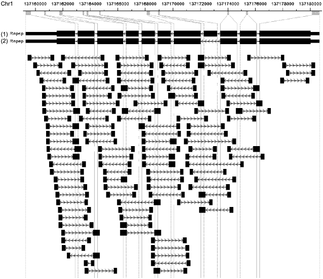
Figure 6: Visualization of RNA-Seq read pairs mapped to the mouse gene Rnpep in the CisGenome Browser (see Jiang et al., 2010). From top to bottom: genomic coordinates, gene structure where exons are magnified for better visualization, read pairs mapped to the gene. Reads are 32 bp at each end. A read that spans a junction between two exons is represented by a wider box.

Because more than $99\%$ of the data have an inferred length between $73$ bp and $324$ bp, reads outside of this range are not considered in subsequent analysis for this example, as it is likely these reads come from unannotated isoforms. This resulted in 27,118 (about $1\%$) read pairs being excluded and the rest 2,762,428 (denoted as $n$ below) read pairs were used in the computation.

The mouse gene Rnpep is used to demonstrate the computation of minimal sufficient statistics. Rnpep has an alternatively spliced exon which gives rise to two different isoforms (see Figure 6). The gene itself is an amino peptidase, meaning that it is used to degrade proteins in the cell. After mapping, 116 read pairs were assigned to this gene, out of which 113 read pairs were used in the computation after outlier removal. Figure 6 presents the positions where the reads are mapped. The gene was picked because it has two alternatively spliced isoforms with a structure that makes distinguishing reads from each isoform challenging, and because the number of reads was small enough to visualize all of them in a simple figure.

Table 2: Single end read categories for Rnpep

Category ID	Sampling rate vector	Read count
1	$[4{,}242n,4{,}242n]$	216
2	$[296n,0]$	010
3	$[0,62n]$	000

5.1 Uniform Sampling Model

Any paired end read experiment can be treated as a single end read experiment by taking each paired end read and treating it as two distinct single end reads, one from each side of the pair. In this, the 113 paired end reads become 226 single end reads (without pairing information).

In the uniform sampling model, for either isoform, the sampling rate vector for each read $s_{j}$ can take at most two values: $2n$ when the isoform can generate read $j$ and $0$ when it cannot. Because there are only two isoforms, one of which (isoform $2$) excludes one of the exons of the other (isoform $1$), it is evident that in the uniform sampling model, there are only three categories for the two isoforms.

The total length of isoform $1$ is $2{,}300$. The total length of isoform $2$ is $2{,}183$. Hence, computing $a_{i,j}$ by summing over the sampling rate vectors of the reads in the same category, the three categories can be represented by their sampling vectors: $[4{,}242n,4{,}242n]$, $[296n,0]$, $[0,62n]$. Using minimal sufficient statistics reduces the data from a vector representing counts on the $2{,}300$ possible reads $s_{j}$ from the two isoforms to the $3$ minimal sufficient statistics which are counts on these categories.

The three categories representing minimal sufficient statistics are tabulated in Table 2. Each category refers to a group of reads that is generated by a particular set of isoforms. For example, category 1 consists of reads generated by both isoforms and category 3 consists of reads generated by isoform 2 only. Using these statistics to solve the optimization problem (3.5), the MLE for the two isoforms is $[\hat{\theta}_{1},\hat{\theta_{2}}]=[15.47,2.70]$. Bayesian credible intervals for these estimates can be obtained by sampling from the posterior space of the parameters (as outlined in Jiang and Wong (2009)), the marginal $95\%$ credible intervals for $\theta_{1}$ and $\theta_{2}$ are $(7.89,18.81)$ and $(0.25,10.83)$, respectively.

5.2 Insert Length Model

To visualize how the insert length model can be used to produce potentially stronger statistical inference as compared to the uniform sampling model, consider Figure 6. Each paired end read is depicted by two boxes with arrows joining pairs of reads. The direction of the arrows represent which side of the read was sequenced first. For those interested, the direction of the arrows in the Rnpep gene itself indicates the transcriptional direction of the gene in genomic coordinates, although this concept can be ignored for the purposes here. Note that there is no direct evidence that isoform $2$ is present in the sample, as no read crosses the junction between the two exons which are adjacent in isoform $2$ but not in isoform $1$. There is direct evidence of the presence of isoform $1$, for example, as depicted in the fifth read from the left in the first row which directly crosses a junction between two exons only adjacent in isoform $1$.

Table 3: Paired read categories for Rnpep

Category ID	Sampling rate vector	Read count
001	$[1{,}681.82n,1{,}681.82n]$	95
002	$[294.60n,0]$	10
003	$[0,245.80n]$	02
00⋮	⋮	0⋮
138	$[0.0057n,0.0018n]$	00

Because of the small gap between exons in the figure, reads spanning exons will be slightly longer than reads not spanning exons. Also, some inserts are very short, and absence of the arrow connecting two reads indicates that the entire insert has been fully sequenced. Note that several of the reads spanning the alternatively spliced exon are exceedingly long. This suggests that such reads are actually generated from isoform $2$ rather than isoform $1$. If such reads are generated from isoform $2$, they would likely have a smaller insert length than the inferred insert length when generated by isoform $1$, which are the lengths depicted in the figure. Because the empirical insert length distribution has its only mode near $250$ bp, conditional on observing the $6$th and $7$th reads from the top of the figure spanning the alternatively spliced exon, the read is more likely to come from isoform $2$. Thus, there is indirect evidence of the presence of isoform $2$ in the sample.

Such indirect evidence is utilized by the insert length model; the model produces quantitative estimates of the relative abundance of the two isoforms. As will be seen in the next section, the abundance estimates from the insert length model have larger Fisher information than the estimates from the uniform sampling model.

In the insert length model, each of the possible insert lengths where $q(\cdot)$ has support produce a unique read $s_{j}$ yielding a total of $569{,}205$ possible reads from the two isoforms. The maximal collapsing produces a total of 138 categories, some of which are represented in Table 3. For intuition, all of the reads with a fixed insert length where both ends fall in the leftmost 7 or rightmost 3 exons of Rnpep will be in the same category, as they have the same probability of being sampled.

Using the minimal sufficient statistics, the MLE is computed to be $[\hat{\theta}_{1},\hat{\theta}_{2}]=[16.73,3.43]$. The marginal $95\%$ credible intervals for $\theta_{1}$ and $\theta_{2}$ are $(11.22,21.02)$ and $(1.03,9.29)$, respectively. The computed marginal $95\%$ credible intervals for $\theta_{1}$ and $\theta_{2}$ are nonoverlapping, whereas in the single end read model, one cannot conclude that the expression of isoforms $1$ and $2$ differ. Further, the insert length model has slightly smaller marginal credible intervals for each parameter.

This example suggests that although the uniform sampling model for single end reads has twice the sample size compared with the insert length model for paired end reads, the insert length model actually provides estimates with smaller standard errors than those generated by the uniform sampling model, because the insert length model can utilize the extra information from the insert sizes of the reads. This difference can be quantified by analyzing the Fisher information of each model, the subject of Section 6.

5.3 Practical Implementation Issues

In general, to apply Theorem 3, one needs to enumerate all the read types before collapsing, as shown in the example of mouse gene Rnpep. This might be a time consuming step, especially when the number of read types is large. In practice, however, under some suitable sampling rate models (which include both our uniform model and insert length model), it is sufficient to enumerate only the read types that have at least one read being mapped. This can reduce the computation when the number of mapped reads for the gene is small, or, in other words, when the gene is lowly expressed.

To see how this works, rearrange the right-hand side of equation (2) as follows:

$$f_{{\theta}}(n_{1},n_{2},\ldots,n_{J})$$

$$\quad={\prod_{j=1}^{J}\frac{(\theta\cdot a_{j})^{n_{j}}e^{-{\theta\cdot a_{j}}}}{n_{j}!}}$$

$$\quad={\prod_{n_{j}>0}\frac{(\theta\cdot a_{j})^{n_{j}}}{n_{j}!}\prod_{n_{j}=0}\frac{(\theta\cdot a_{j})^{n_{j}}}{n_{j}!}\prod_{j=1}^{J}e^{-{\theta\cdot a_{j}}}}$$

(9)

$$\quad={\prod_{n_{j}>0}\frac{(\theta\cdot a_{j})^{n_{j}}}{n_{j}!}\prod_{j=1}^{J}e^{-{\theta\cdot a_{j}}}}$$

$$\quad={\prod_{n_{j}>0}\frac{(\theta\cdot a_{j})^{n_{j}}}{n_{j}!}\prod_{j=1}^{J}{e^{-{\sum_{i=1}^{I}\theta_{i}{a_{i,j}}}}}}$$

$$\quad={\prod_{n_{j}>0}\frac{(\theta\cdot a_{j})^{n_{j}}}{n_{j}!}\prod_{i=1}^{I}{e^{-\theta_{i}\sum_{j=1}^{J}{a_{i,j}}}}},$$

where only the term ${\sum_{j=1}^{J}{a_{i,j}}}$ depends on the sampling rates of read types with read counts $n_{j}=0$. Therefore, if we can compute this term withoutknowing each particular sampling rate $a_{i,j}$, the enumeration of all the read types is no longer necessary. Fortunately, it is possible under some suitable sampling rate models, including both our uni-form model and insert length model. For example, in the uniform model, ${\sum_{j=1}^{J}{a_{i,j}}}=n(l_{i}-r+1)$, where $n$ is the total number of mapped reads, $l_{i}$ is the length of transcript $i$ and $r$ is the read length. Similarly,in the insert length model, ${\sum_{j=1}^{J}{a_{i,j}}}=\break{\sum_{q(r)>0}nq(r)(l_{i}-r+1)}$.

Using this trick, we can take only the read types with at least one read being mapped and collapse them to categories $C_{1},C_{2},\ldots,C_{K}$. Accordingly, the optimization problem [equation (3.5)] is reduced to

$$\mbox{maximize}\quad{n}^{T}\log({A^{T}}{\theta})-W^{T}\theta$$

(10)

$$\quad\mbox{s.t. }{\theta}\geq 0,$$

where ${n}$ is a $K\times 1$ column vector for the collapsed read counts for categories $C_{1},C_{2},\ldots,C_{K}$, $A$ is a $I\times K$ matrix for the collapsed sampling rates and ${\theta}$ is the isoform abundance vector. $W$ is a $I\times 1$ vector with the $i$th element $W_{i}$=$\sum_{j=1}^{J}{a_{i,j}}$ computed based on the corresponding sampling rate model.

In a more complex sampling rate model, for example, when $a_{i,j}$ depends on the particular nucleotide sequence of read $s_{j}$, the optimization problem [equation (5.3)] can still be solved. However, all the read types (including the read types with $n_{j}=0$) will have to be enumerated and each sampling rate $a_{i,j}$ will have to be computed.

6 Information Theoretic Analysis

Many considerations impact the choice of sequencing protocol in an experimental design. One such choice is relative cost of sequencing. In this case, the experimentalist may be interested in choosing the sequencing protocol (paired end or single end) that provides the best estimate of isoform abundance at the least relative cost. This section outlines the statistical argument for why, in typical situations, paired end sequencing can produce better estimates of transcript abundance compared to single end sequencing at a fixed number of sequenced nucleotides (cost). The theoretical analysis aims to show that for the same number of sequenced nucleotides, the Fisher information in the insert length model is more than double the Fisher information in the single end read model. Since estimates in RNA-Seq are maximum likelihood estimators, their variance of the estimator converges to the reciprocal of the Fisher information. Thus, larger Fisher information produces estimators with improved accuracy.

6.1 Theoretical Analysis

Consider the following quite simple example showing the increase in information as the fraction of reads unique to each isoform grows:

Example 4.

Continuing Example $1$, supposethat isoform 1 and isoform 2 have Poisson rate parameters $\theta_{1}$ and $\theta_{2}$, respectively, where $\theta_{2}=1-\theta_{1}$ and probability $0<\alpha,\beta<1$, respectively, of producing a read unique to the isoform. Let $n_{1}$ be the reads unique to $1$, $n_{2}$ the reads unique to $2$ and $n_{3}$ the reads which cannot be distinguished between the isoforms. Assume there are $n$ total reads in the sample, and assume there is uniform fragmentation which gives rise to three categories:

$$n_{1} = \operatorname{Po}(n\alpha\theta_{1}),$$

$$n_{2} = \operatorname{Po}(n\beta\theta_{2}),$$

$$n_{3} = \operatorname{Po}\bigl{(}n\bigl{(}(1-\alpha)\theta_{1}+(1-\beta)\theta_{2}\bigr{)}\bigr{)}.$$

Fix $\alpha<\beta$ as known and compute the information in this distribution with $\theta_{1}$ as the unknown parameter as a function of $\alpha$ using the definition that the information is equal to the variance of the derivative of the log likelihood with respect to $\theta_{1}$:

$$I(\theta_{1}) = \operatorname{var}{\biggl{(}\frac{n_{1}}{\theta_{1}}-\frac{n_{2}}{\theta_{2}}+\frac{n_{3}(\bar{\alpha}-\bar{\beta})}{\theta_{1}(\bar{\alpha}-\bar{\beta})+\bar{\beta}}\biggr{)}}$$

$$= n\biggl{(}\frac{\alpha}{\theta_{1}}+\frac{\beta}{\theta_{2}}+\frac{(\bar{\alpha}-\bar{\beta})}{\theta_{1}(\bar{\alpha}-\bar{\beta})+\bar{\beta}}\biggr{)},$$

where $\bar{x}=1-x$. Thus, $\bar{\alpha}-\bar{\beta}=\beta-\alpha$, and $\delta:=\beta-\alpha$ and $\alpha$ are re-parameterizations of $\beta,\alpha$. The last equation shows that the partial derivatives of the information with respect to $\alpha$ and with respect to $\delta$ are positive.

Note that in the example above, no generality is lost by assuming $\beta>\alpha$ since $\theta_{1}$ and $\theta_{2}$ can be interchanged with no effect on the model.

To see that for a fixed cost of sequencing (number of sequenced nucleotides) the statistical model produced by paired end sequencing has more information than single end sequencing, it is necessary to show that the information obtained by twice as many single end reads in a single end sequencing experiment is smaller than that obtained by a paired end sequencing experiment. Such a comparison necessarily depends on each gene, its isoforms and their relative abundance. The computation of the Fisher information for a typical such example is presented below, and the computation shows that the example easily generalizes to other configurations of isoforms.

Example 5.

Continuing the running example, consider reads of length $r=100$ bp and paired end insert size $x=200$ bp in the schematic of three exons in Figure 1, where the length of exons $1$ and $3$ is $500$ bp and exon $2$ is $e=50$ bp (see Figure 7).

Figure 7: A model gene for the study of Fisher information and accuracy of the single end and insert length models.

For a single end read experiment, $\alpha_{s}$ is the probability that a read includes any part of the included exon (i.e., uniquely identifies isoform 2), so for the read length of $r$,

$$\alpha_{s}=\frac{r-1+e}{1{,}000+e-r+1}$$

and $\beta_{s}$ is the probability that a read includes any part of the spliced junction (i.e., uniquely identifies isoform 1) so

$$\beta_{s}=\frac{r-1}{1{,}000-r+1}.$$

For a paired end read experiment, with $x$ the insert length, $\alpha_{p}$, the probability that a read uniquely identifies the second isoform, is

$$\alpha_{p}=\frac{e+x-1}{1{,}000+e-x+1},$$

and $\beta_{p}$, the probability that a read uniquely identifies the first isoform, is

$$\beta_{p}=\frac{x-1}{1{,}000-x+1}.$$

For a concrete example, suppose $\theta_{1}=2\theta_{2}$. Assume further that there are twice as many single end reads (a sample size of $2n$) compared to the $n$ reads in a paired end run:

$$I_{s}:=2n\biggl{(}\frac{3}{2}{\alpha_{s}}+3{\beta_{s}}+\frac{(\bar{\alpha_{s}}-\bar{\beta_{s}})}{(2/3)(\bar{\alpha_{s}}-\bar{\beta_{s}})+\bar{\beta_{s}}}\biggr{)},$$

and the information in a paired end run for a fixed insert size is

$$I_{p}:=n\biggl{(}\frac{3}{2}{\alpha_{p}}+3{\beta_{p}}+\frac{(\bar{\alpha_{p}}-\bar{\beta_{p}})}{(2/3)(\bar{\alpha_{p}}-\bar{\beta_{p}})+\bar{\beta_{p}}}\biggr{)}.$$

Plugging in numbers $x=200$, $e=50$, and $r=30$ gives

$$\frac{I_{s}}{I_{p}}=\frac{0.31}{1.12}=0.28.$$

In other words, in the insert length model, the maximum likelihood estimator of $\theta_{1}$ has asymptotic variance roughly $3$ times larger in the single end read experiment than in the paired end experiment.

Of course, this ratio will change if the parameters change. For instance, $I_{s}/I_{p}=0.63$ if $x=200$, $e=50$ and $r=70$; $I_{s}/I_{p}=0.47$ if $x=200$, $e=100$ and$r=50$.

The next section gives simulation results for a related example.

6.2 Simulation Study

Simulations were used to study the following questions: (1) the quality of the proposed model at estimating isoform-specific gene expression, especially when the insert length is variable, and (2) whether abundance estimates from paired end reads are more reliable than abundance estimates from single end reads.

To address these questions, reads were simulated from a “hard case” where a gene has three exons of lengths 500 bp, 50 bp and 500 bp, respectively (see Figure 7); the middle exon can be skipped, producing two different isoforms of the gene. Since the middle exon is short, this case has been shown to be difficult for isoform-specific gene expression estimation in Jiang and Wong (2009).

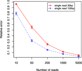
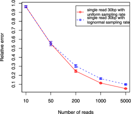
(a)	(b)
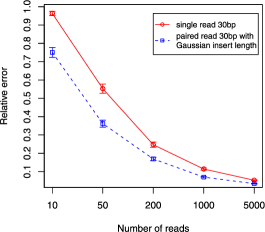
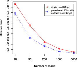
(c)	(d)

Figure 8: Relative error of different read generation models. X axis is the sample size, that is, the number of reads that is generated in each simulation experiment. Y axis is the mean relative error based on $200$ simulation experiments. The error bars give the standard errors of the sample means. In the figures, single 30 bp reads generated with uniform sampling rate (solid curves) are compared to (dashed curves) (a) single 100 bp reads, (b) single 30 bp reads generated with lognormal sampling rate, (c) paired end 30 bp reads generated with Gaussian insert size and (d) paired end 30 bp reads generated with uniform insert size. When compared with $n$ (e.g., $5{,}000$) single end reads, $n/2$ (i.e., $2{,}500$) pairs of paired end reads were used.

In the simulation, the two isoforms were assumed to have equal abundance. Reads were simulated using different models and parameters described in detail below and estimate isoform abundances as described in Section 3.5. The relative error of estimation was computed based on the empirical relative $L^{2}$ loss:

$$\frac{\|{\theta}-{\hat{\theta}}\|_{2}}{\|\theta\|_{2}} = \frac{\sqrt{(\theta_{1}-\hat{\theta}_{1})^{2}+(\theta_{2}-\hat{\theta}_{2})^{2}}}{\sqrt{\theta_{1}^{2}+\theta_{2}^{2}}}$$

$$= \frac{\sqrt{(1/2-\hat{\theta}_{1})^{2}+(1/2-\hat{\theta}_{2})^{2}}}{\sqrt{2}/2},$$

where ${\theta}=[\theta_{1},\theta_{2}]=[\frac{1}{2},\frac{1}{2}]$ is the true isoform abundance vector, and ${\hat{\theta}}=[\hat{\theta}_{1},\hat{\theta}_{2}]$ is the estimated isoform abundance vector after normalization so that $\hat{\theta}_{1}+\hat{\theta}_{2}=1$. Each simulation experiment was re-peated $200$ times to get the sample mean and standard error of the relative error.

6.2.1 Simulating single end reads with uniformsampling

To explore the quality of estimation in the uniform sampling approach, single end reads with length 30 bp using the uniform sampling model were generated. Five separated experiments were performed to investigate the effect of sample size on the estimation procedure using sample sizes of $10$, $50$, $200$, $1{,}000$ and $5{,}000$, respectively. The solid curve in Figure 8(a) gives the sample mean and standard error of the relative error. It is clear that relative error decreases as the sample size increases.

To examine whether longer reads can provide better estimates, all the simulation experiments were repeated with read length $100$ bp. Figure 8(a) shows the comparison between read lengths of $30$ bp and $100$ bp. As expected, $100$ bp reads produce smaller error than $30$ bp reads.

6.2.2 Simulating single end reads with nonuniform sampling

In real UHTS data, the read distribution is not uniform. To evaluate how well the RNA-Seq methodology performs in this regime, simulations were performed where the positions of reads were sampled from a log-normal distribution. Specifically, up to a scalar multiple, the true sampling rates $a_{i,j}$ are independently and identically distributed random variables which follow log-normal distribution with mean $\mu=0$ and standard deviation $\sigma=1$.

Figure 8(b) gives the comparison between reads that were sampled from uniform distribution and reads that were sampled from log-normal distribution The figure shows that nonuniform reads produce estimates which appear consistent, albeit with larger error than with uniform reads.

6.2.3 Simulating paired end reads

This section investigates whether, in simulation, paired end reads can provide more information than single end reads. When insert lengths do not have a simple distribution, closed form expressions for the information are difficult to obtain. Simulation studies are thus important tools for analyzing such situations. For this purpose, paired end reads of length $30$ bp with insert size following a normal distribution with mean $\mu=200$ bp and standard deviation $\sigma=20$ bp were generated. For a given insert size, read pairs were generated using a uniform sampling model. Figure 8(c) shows that the paired end reads produce smaller errors than single end reads with the same number of sequenced nucleotides: to make the comparison comparable on the level of total sequenced bases, $n/2$ pairs of paired end reads were used when compared with $n$ single end reads.

When the insert size was generated using a uniform distribution, for example, the effective insert size is uniform within $200\pm 20$ bp, similar results were produced [see Figure 8(d)]. Comparing Figure 8(d) with Figure 8(a) shows that paired end 30 bp reads produce similarly accurate estimates as 100 bp single end reads, which means that, on average, paired end reads provide more information per nucleotide being sequenced.

6.2.4 Simulating with other parameters

We also performed simulations with other settings of parameters, for instance, with read length 70 bp, with true isoform expression vector $(0.1,0.9)$ or with exon lengths (500 bp, 200 bp, 500 bp). The results are shown in Figure 9. In all these simulations, the advantage of paired end sequencing over single end sequencing is obvious for moderate sampling ($50\leq n\leq 1{,}000$), as in typical cases for sequencing data.

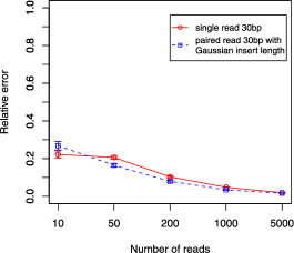
(a)	(b)
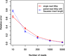
c

Figure 9: Relative error of single end reads (solid curves) and paired end reads (dashed curves) with different settings of parameters: (a) 70 bp reads, true isoform expression vector $(0.5,0.5)$ (b) 30 bp reads, true isoform expression vector $(0.1,0.9)$ (c) 30 bp reads, true isoform expression vector $(0.5,0.5)$, exon lengths (500 bp, 200 bp, 500 bp). When compared with $n$ (e.g., $5{,}000$) single end reads, $n/2$ (i.e., $2{,}500$) pairs of paired end reads were used.

7 Discussion

The insert length model presented in this paper is a flexible statistical tool. The model has the capacity to accommodate oriented reads from Illumina data and to model fragment specific biases in the probability of each fragment being sequenced. In Section 3.2 the model has been derived when the experimental step of fragmentation is assumed to be approximated by a Poisson point process, and a transcript is assumed to be retained in the sample in proportion to the fraction of transcripts of its length estimated after sequencing. These assumptions are at once simplifying and realistic. As experimental protocols improve, it is likely they will better model RNA-Seq data.

At the current time, several improvements may be made to the model to increase its accuracy. First, the read sampling rate is undoubtedly nonuniform, as it depends on biochemical properties of the sample and fragmentation process as experimental studies have highlighted (see Ingolia et al. (2009); Vega et al. (2009), and Quail et al. (2008)). This effect becomes more apparent for longer fragments such as those used in paired end library preparation. Explicit models for the sampling rates are difficult to obtain, but doing so is an area of future research. Recent research (see Hansen, Brenner and Dudoit (2010); Li, Jiang and Wong (2010)) has shown that the nonuniformity can be modeled and estimated quite well from the data. It may be possible to combine these models with our approach to improve the estimation performance.

Statistical tests of the reproducibility of the nonuniformity of reads shows a consistent sequence specific bias across biological and technical replicates of a gene. This effect could be due to bias in RNA fragmentation, bias in other biochemical sample preparation steps or boundary effects when a gene of fixed length is fragmented. The last cause of bias can be modeled using Monte Carlo simulations of a fixed length mRNA sequence subject to a Poisson fragmentation process and incorporated into the insert length model.

Similarly, the fragmentation and filtering steps have not been explicitly modeled in the insert length model presented here. Rather, the probability mass function of read lengths, what is necessary for defining the model, has been estimated empirically. Improvements to the model could be made by increasing the precision of the estimate of the probability mass function of read lengths, for example, by simulating a fragmentation and filtering process by Monte Carlo and matching the output of the simulations to the empirical distribution function $q(\cdot)$. If such modeling were desired, as described in Section 3.2, the effects could be easily incorporated into the insert length model. On the other hand, as experimental protocols improve, they may reduce this bias and increase the accuracy of the insert length model as presented in this paper.

In reality, sequencing mapping is another step that may affect the analysis. For instance, some reads cannot be mapped because of sequencing errors and some can be mapped to multiple places. We have not focused on the issue of mapping fidelity because we restrict attention to the reads which did map uniquely. We are also not taking into account mapping errors which themselves require statistical modeling. We have chosen not to model these errors partly because some mapping errors are platform-dependent (i.e., different sequencing errors tend to be made by the Illumina vs. other platforms).

In some applications, the parameters of interest to biologists are not the RPKMs for isoforms 1 and 2, but rather the relative expression ratio of both isoforms. One way to estimate the ratio is to reparameterize the problem with $\theta_{1}$ as a first parameter and a second parameter $\mu=\theta_{1}/\theta_{2}$. The reparameterization will make the model no longer linear in the parameters, therefore harder to solve. Also, the choice of $\mu$ is not straightforward when there are 3 or more isoforms. An easier way is to estimate $\mu$ indirectly after estimating $\theta_{1}$ and $\theta_{2}$.

We believe that technological improvements that produce longer read lengths will not diminish the relevance of the insert length model. Paired end models will be relevant at least until read lengths are comparable to the length of each transcript, and perhaps longer for reasons of cost. Since many transcripts are larger than $10^{4}$ nucleotides, and longer in some important cases, such a time is unlikely to occur in the next few years. Further, longer insert lengths and reads combined with the insert length model in this paper will aid in discrimination of complex isoforms and estimation of isoform-specific poly-A tail lengths. Thus, we do not foresee any imminent obsolescence of this model.

While the model developed in this paper has the potential for great use and extends current methodology for isoform-specific estimation, the model assumes that the complete set of isoforms of a gene have been annotated. De novo discovery of isoforms from a sample is an important and difficult statistical problem that we have not addressed in this paper. Another shortcoming of the model is that in order for statistical inference to be accurate, with the current short read technology, the number of isoforms should be relatively small (e.g., 2–5). We expect these challenges to motivate methodological development in the field of RNA-Seq in the coming years.

In conclusion, this paper has presented a statistical model for RNA-Seq experiments which provides estimates for isoform specific expression. Finding such estimates is difficult using microarray technology, focusing interest in UHTS to address this question. In addition to modeling, the paper has presented an in-depth statistical analysis. By using the classical statistical concept of minimal sufficiency, a computationally feasible solution to isoform estimation in RNA-Seq is provided. Further, statistical analysis quantifies the perceived gain in experimental efficiency from using paired end rather than single end read data to provide reliable isoform specific gene expression estimates. To the best of our knowledge, this is the first statistical model for answering this question.

References

- Bullard et al. (2010) {barticle}[auto:STB—2010-11-18—09:18:59] \bauthor\bsnmBullard, \bfnmJ. H.\binitsJ. H., \bauthor\bsnmPurdom, \bfnmE.\binitsE., \bauthor\bsnmHansen, \bfnmK. D.\binitsK. D. and \bauthor\bsnmDudoit, \bfnmS.\binitsS. (\byear2010). \btitleEvaluation of statistical methods for normalization and differential expression in mRNA-Seq experiments. \bjournalBMC Bioinformatics \bvolume11. \endbibitem
- Casella and Berger (2002) {bbook}[auto:STB—2010-11-18—09:18:59] \bauthor\bsnmCasella, \bfnmG.\binitsG. and \bauthor\bsnmBerger, \bfnmR.\binitsR. (\byear2002). \btitleStatistical Inference, \bedition2nd ed. \bpublisherThomson Learning, \baddressDuxbury. \endbibitem
- Chi (2008) {barticle}[auto:STB—2010-11-18—09:18:59] \bauthor\bsnmChi, \bfnmK. R.\binitsK. R. (\byear2008). \btitleThe year of sequencing. Nature \bjournalMethods \bvolume5 \bpages11–14. \endbibitem
- Hansen, Brenner and Dudoit (2010) {barticle}[auto:STB—2010-11-18—09:18:59] \bauthor\bsnmHansen, \bfnmK. D.\binitsK. D., \bauthor\bsnmBrenner, \bfnmS. E.\binitsS. E. and \bauthor\bsnmDudoit, \bfnmS.\binitsS. (\byear2010). \btitleBiases in illumina transcriptome sequencing caused by random hexamer priming. \bjournalNucleic Acids Res. \bvolume38 \bpagese131. \endbibitem
- Hansen et al. (2009) {bmisc}[auto:STB—2010-11-18—09:18:59] \bauthor\bsnmHansen, \bfnmK. D.\binitsK. D., \bauthor\bsnmLareau, \bfnmL. F.\binitsL. F., \bauthor\bsnmBlanchette, \bfnmM.\binitsM., \bauthor\bsnmGreen, \bfnmR. E.\binitsR. E., \bauthor\bsnmMeng, \bfnmQ.\binitsQ., \bauthor\bsnmRehwinkel, \bfnmJ.\binitsJ., \bauthor\bsnmGallusser, \bfnmF. L.\binitsF. L., \bauthor\bsnmIzaurralde, \bfnmE.\binitsE., \bauthor\bsnmRio, \bfnmD. C.\binitsD. C., \bauthor\bsnmDudoit, \bfnmS.\binitsS. and \bauthor\bsnmBrenner, \bfnmS. E.\binitsS. E. (\byear2009). \bhowpublishedGenome-wide identification of alternative splice forms down-regulated by nonsense-mediated mRNA decay in Drosophila. PLoS Genetics 5 e1000525. \endbibitem
- Hiller et al. (2009) {barticle}[auto:STB—2010-11-18—09:18:59] \bauthor\bsnmHiller, \bfnmD.\binitsD., \bauthor\bsnmJiang, \bfnmH.\binitsH., \bauthor\bsnmXu, \bfnmW.\binitsW. and \bauthor\bsnmWong, \bfnmW. H.\binitsW. H. (\byear2009). \btitleIdentifiability of isoform deconvolution from junction arrays and RNA-Seq. \bjournalBioinformatics \bvolume25 \bpages3056–3059. \endbibitem
- Ingolia et al. (2009) {barticle}[auto:STB—2010-11-18—09:18:59] \bauthor\bsnmIngolia, \bfnmN. T.\binitsN. T., \bauthor\bsnmGhaemmaghami, \bfnmS.\binitsS., \bauthor\bsnmNewman, \bfnmJ. R. S.\binitsJ. R. S. and \bauthor\bsnmWeissman, \bfnmJ. S.\binitsJ. S. (\byear2009). \btitleGenome-wide analysis in vivo of translation with nucleotide resolution using ribosome profiling. \bjournalScience \bvolume324 \bpages218–223. \endbibitem
- Jiang and Wong (2008) {barticle}[auto:STB—2010-11-18—09:18:59] \bauthor\bsnmJiang, \bfnmH.\binitsH. and \bauthor\bsnmWong, \bfnmW. H.\binitsW. H. (\byear2008). \btitleSeqmap: Mapping massive amount of oligonucleotides to the genome. \bjournalBioinformatics \bvolume24 \bpages2395–2396. \endbibitem
- Jiang and Wong (2009) {barticle}[auto:STB—2010-11-18—09:18:59] \bauthor\bsnmJiang, \bfnmH.\binitsH. and \bauthor\bsnmWong, \bfnmW. H.\binitsW. H. (\byear2009). \btitleStatistical inferences for isoform expression in RNA-Seq. \bjournalBioinformatics \bvolume25 \bpages1026–1032. \endbibitem
- Jiang et al. (2010) {barticle}[auto:STB—2010-11-18—09:18:59] \bauthor\bsnmJiang, \bfnmH.\binitsH., \bauthor\bsnmWang, \bfnmF.\binitsF., \bauthor\bsnmDyer, \bfnmN. P.\binitsN. P. and \bauthor\bsnmWong, \bfnmW. H.\binitsW. H. (\byear2010). \btitleCisgenome browser: A flexible tool for genomic data visualization. \bjournalBioinformatics \bvolume26 \bpages1781–1782. \endbibitem
- Langmead et al. (2009) {barticle}[auto:STB—2010-11-18—09:18:59] \bauthor\bsnmLangmead, \bfnmB.\binitsB., \bauthor\bsnmTrapnell, \bfnmC.\binitsC., \bauthor\bsnmPop, \bfnmM.\binitsM. and \bauthor\bsnmSalzberg, \bfnmS.\binitsS. (\byear2009). \btitleUltrafast and memory-efficient alignment of short DNA sequences to the human genome. \bjournalGenome Biol. \bvolume10 \bpagesR25. \endbibitem
- Lehmann (1998) {bbook}[mr] \bauthor\bsnmLehmann, \bfnmE. L.\binitsE. L. (\byear1998). \btitleTheory of Point Estimation, \bedition2nd ed. \bpublisherSpringer, \baddressNew York. \endbibitem
- Li, Jiang and Wong (2010) {barticle}[auto:STB—2010-11-18—09:18:59] \bauthor\bsnmLi, \bfnmJ.\binitsJ., \bauthor\bsnmJiang, \bfnmH.\binitsH. and \bauthor\bsnmWong, \bfnmW. H.\binitsW. H. (\byear2010). \btitleModeling non-uniformity in short-read rates in RNA-Seq data. \bjournalGenome Biol. \bvolume11 \bpagesR50. \endbibitem
- Maher et al. (2009) {barticle}[auto:STB—2010-11-18—09:18:59] \bauthor\bsnmMaher, \bfnmC. A.\binitsC. A., \bauthor\bsnmKumar-Sinha, \bfnmC.\binitsC., \bauthor\bsnmCao, \bfnmX.\binitsX., \bauthor\bsnmKalyana-Sundaram, \bfnmS.\binitsS., \bauthor\bsnmHan, \bfnmB.\binitsB., \bauthor\bsnmJing, \bfnmX.\binitsX., \bauthor\bsnmSam, \bfnmL.\binitsL., \bauthor\bsnmBarrette, \bfnmT.\binitsT., \bauthor\bsnmPalanisamy, \bfnmN.\binitsN. and \bauthor\bsnmChinnaiyan, \bfnmA. M.\binitsA. M. (\byear2009). \btitleTranscriptome sequencing to detect gene fusions in cancer. \bjournalNature \bvolume458 \bpages97–101. \endbibitem
- McCullagh and Nelder (1989) {bbook}[mr] \bauthor\bsnmMcCullagh, \bfnmP.\binitsP. and \bauthor\bsnmNelder, \bfnmJ. A.\binitsJ. A. (\byear1989). \btitleGeneralized Linear Models, \bedition2nd ed. \bpublisherChapman & Hall, \baddressBoca Raton. \bidmr=0727836 \bptnotecheck year \endbibitem
- Mortazavi et al. (2008) {barticle}[auto:STB—2010-11-18—09:18:59] \bauthor\bsnmMortazavi, \bfnmA.\binitsA., \bauthor\bsnmWilliams, \bfnmB. A.\binitsB. A., \bauthor\bsnmMcCue, \bfnmK.\binitsK., \bauthor\bsnmSchaeffer, \bfnmL.\binitsL. and \bauthor\bsnmWold, \bfnmB.\binitsB. (\byear2008). \btitleMapping and quantifying mammalian transcriptomes by RNA-Seq. \bjournalNature Methods \bvolume5 \bpages621–628. \endbibitem
- Pan et al. (2008) {barticle}[auto:STB—2010-11-18—09:18:59] \bauthor\bsnmPan, \bfnmQ.\binitsQ., \bauthor\bsnmShai, \bfnmO.\binitsO., \bauthor\bsnmLee, \bfnmL. J.\binitsL. J., \bauthor\bsnmFrey, \bfnmB. J.\binitsB. J. and \bauthor\bsnmBlencowe, \bfnmB. J.\binitsB. J. (\byear2008). \btitleDeep surveying of alternative splicing complexity in the human transcriptome by high-throughput sequencing. \bjournalNature Genet. \bvolume40 \bpages1413–1415. \endbibitem
- Pruitt, Tatusova and Maglott (2005) {barticle}[auto:STB—2010-11-18—09:18:59] \bauthor\bsnmPruitt, \bfnmK. D.\binitsK. D., \bauthor\bsnmTatusova, \bfnmT.\binitsT. and \bauthor\bsnmMaglott, \bfnmD. R.\binitsD. R. (\byear2005). \btitleNCBI reference sequence (RefSeq): A curated non-redundant sequence database of genomes, transcripts and proteins. \bjournalNucleic Acids Res. \bnote33 D501–D504. \endbibitem
- Quail et al. (2008) {barticle}[auto:STB—2010-11-18—09:18:59] \bauthor\bsnmQuail, \bfnmM. A.\binitsM. A., \bauthor\bsnmKozarewa, \bfnmI.\binitsI., \bauthor\bsnmSmith, \bfnmF.\binitsF., \bauthor\bsnmScally, \bfnmA.\binitsA., \bauthor\bsnmStephens, \bfnmP. J.\binitsP. J., \bauthor\bsnmDurbin, \bfnmR.\binitsR., \bauthor\bsnmSwerdlow, \bfnmH.\binitsH. and \bauthor\bsnmTurner1, \bfnmD. J.\binitsD. J. (\byear2008). \btitleA large genome center’s improvements to the illumina sequencing system. \bjournalNature Methods \bvolume5 \bpages1005–1010. \endbibitem
- She, Hubbell and Wang (2009) {barticle}[auto:STB—2010-11-18—09:18:59] \bauthor\bsnmShe, \bfnmY.\binitsY., \bauthor\bsnmHubbell, \bfnmE.\binitsE. and \bauthor\bsnmWang, \bfnmH.\binitsH. (\byear2009). \btitleResolving deconvolution ambiguity in gene alternative splicing. \bjournalBMC Bioinformatics \bvolume10. \endbibitem
- Sultan et al. (2008) {barticle}[auto:STB—2010-11-18—09:18:59] \bauthor\bsnmSultan, \bfnmM.\binitsM., \bauthor\bsnmSchulz, \bfnmM. H.\binitsM. H., \bauthor\bsnmRichard, \bfnmH.\binitsH., \bauthor\bsnmMagen, \bfnmA.\binitsA., \bauthor\bsnmKlingenhoff, \bfnmA.\binitsA., \bauthor\bsnmScherf, \bfnmM.\binitsM., \bauthor\bsnmSeifert, \bfnmM.\binitsM., \bauthor\bsnmBorodina, \bfnmT.\binitsT., \bauthor\bsnmSoldatov, \bfnmA.\binitsA., \bauthor\bsnmParkhomchuk, \bfnmD.\binitsD., \bauthor\bsnmSchmidt, \bfnmD.\binitsD., \bauthor\bsnmO’Keeffe, \bfnmS.\binitsS., \bauthor\bsnmHaas, \bfnmS.\binitsS., \bauthor\bsnmVingron, \bfnmM.\binitsM., \bauthor\bsnmLehrach, \bfnmH.\binitsH. and \bauthor\bsnmYaspo, \bfnmM.-L.\binitsM.-L. (\byear2008). \btitleA global view of gene activity and alternative splicing by deep sequencing of the human transcriptome. \bjournalScience \bvolume321 \bpages956–960. \endbibitem
- Trapnell, Pachter and Salzberg (2009) {barticle}[auto:STB—2010-11-18—09:18:59] \bauthor\bsnmTrapnell, \bfnmC.\binitsC., \bauthor\bsnmPachter, \bfnmL.\binitsL. and \bauthor\bsnmSalzberg, \bfnmS. L.\binitsS. L. (\byear2009). \btitleTophat: Discovering splice junctions with RNA-Seq. \bjournalBioinformatics \bvolume25 \bpages1105–1111. \endbibitem
- Trapnell et al. (2010) {barticle}[auto:STB—2010-11-18—09:18:59] \bauthor\bsnmTrapnell, \bfnmC.\binitsC., \bauthor\bsnmWilliams, \bfnmB. A.\binitsB. A., \bauthor\bsnmPertea, \bfnmG.\binitsG., \bauthor\bsnmMortazavi, \bfnmA.\binitsA., \bauthor\bsnmKwan, \bfnmG.\binitsG., \bauthor\bparticlevan \bsnmBaren, \bfnmM. J.\binitsM. J., \bauthor\bsnmSalzberg, \bfnmS. L.\binitsS. L., \bauthor\bsnmWold, \bfnmB. J.\binitsB. J. and \bauthor\bsnmPachter, \bfnmL.\binitsL. (\byear2010). \btitleTranscript assembly and quantification by RNA-Seq reveals unannotated transcripts and isoform switching during cell differentiation. \bjournalNature Biotechnol. \bvolume28 \bpages511–515. \endbibitem
- Vega et al. (2009) {barticle}[auto:STB—2010-11-18—09:18:59] \bauthor\bsnmVega, \bfnmV. B.\binitsV. B., \bauthor\bsnmCheung, \bfnmE.\binitsE., \bauthor\bsnmPalanisamy, \bfnmN.\binitsN. and \bauthor\bsnmSung, \bfnmW.-K.\binitsW.-K. (\byear2009). \btitleInherent signals in sequencing-based chromatin-immunoprecipitation control libraries. \bjournalPLoS ONE \bvolume4 \bpagese5241. \endbibitem
- Wahlstedt et al. (2009) {barticle}[auto:STB—2010-11-18—09:18:59] \bauthor\bsnmWahlstedt, \bfnmH.\binitsH., \bauthor\bsnmDaniel, \bfnmC.\binitsC., \bauthor\bsnmEnstero, \bfnmM.\binitsM. and \bauthor\bsnmOhman, \bfnmM.\binitsM. (\byear2009). \btitleLarge-scale MRNA sequencing determines global regulation of RNA editing during brain development. \bjournalGenome Res. \bvolume19 \bpages978–986. \endbibitem
- Wang et al. (2008) {barticle}[auto:STB—2010-11-18—09:18:59] \bauthor\bsnmWang, \bfnmE. T.\binitsE. T., \bauthor\bsnmSandberg, \bfnmR.\binitsR., \bauthor\bsnmLuo, \bfnmS.\binitsS., \bauthor\bsnmKhrebtukova, \bfnmI.\binitsI., \bauthor\bsnmZhang, \bfnmL.\binitsL., \bauthor\bsnmMayr, \bfnmC.\binitsC., \bauthor\bsnmKingsmore, \bfnmS. F.\binitsS. F., \bauthor\bsnmSchroth, \bfnmG. P.\binitsG. P. and \bauthor\bsnmBurge, \bfnmC. B.\binitsC. B. (\byear2008). \btitleAlternative isoform regulation in human tissue transcriptomes. \bjournalNature \bvolume456 \bpages470–476. \endbibitem
- Zhang et al. (2009) {barticle}[auto:STB—2010-11-18—09:18:59] \bauthor\bsnmZhang, \bfnmW.\binitsW., \bauthor\bsnmDuan, \bfnmS.\binitsS., \bauthor\bsnmBleibel, \bfnmW. K.\binitsW. K., \bauthor\bsnmWisel, \bfnmS. A.\binitsS. A., \bauthor\bsnmHuang, \bfnmR. S.\binitsR. S., \bauthor\bsnmWu, \bfnmX.\binitsX., \bauthor\bsnmHe, \bfnmL.\binitsL., \bauthor\bsnmClark, \bfnmT. A.\binitsT. A., \bauthor\bsnmChen, \bfnmT. X.\binitsT. X., \bauthor\bsnmSchweitzer, \bfnmA. C.\binitsA. C., \bauthor\bsnmBlume, \bfnmJ. E.\binitsJ. E., \bauthor\bsnmDolan, \bfnmM. E.\binitsM. E. and \bauthor\bsnmCox, \bfnmN. J.\binitsN. J. (\byear2009). \btitleIdentification of common genetic variants that account for transcript isoform variation between human populations. \bjournalJ. Human Genetics \bvolume125 \bpages81–93. \endbibitem