Creating Domain Mappings

Abstract

Consider being given a mapping $\varphi:S^{d-1}\overset{1-1}{\underset{onto}{\longrightarrow}}\partial\Omega$, with $\partial\Omega$ the $\left(d-1\right)$-dimensional smooth boundary surface for a bounded open simply-connected region $\Omega$ in $\mathbb{R}^{d}$, $d\geq 2$. We consider the problem of constructing an extension $\Phi:\overline{B}_{d}\overset{1-1}{\underset{onto}{\longrightarrow}}\overline{\Omega}$ with $B_{d}$ the open unit ball in $\mathbb{R}^{d}$. The mapping is also required to be continuously differentiable with a non-singular Jacobian matrix at all points. We discuss ways of obtaining initial guesses for such a mapping $\Phi$ and of then improving it by an iteration method.

1 Introduction

Consider the following problem. We are given

$$\varphi:\partial B_{d}\underset{onto}{\overset{1-1}{\longrightarrow}}\partial\Omega$$ (1)

Notationally, $d\geq 2$, $B_{d}$ is the open unit ball in $\mathbb{R}^{d}$ with boundary $S^{d-1}=\partial B_{d}$, and $\Omega$ is an open, bounded, simply-connected region in $\mathbb{R}^{d}$. We want to construct a continuously differentiable extension

$$\Phi:\overline{B}_{d}\underset{onto}{\overset{1-1}{\longrightarrow}}\overline{\Omega}$$ (2)

such that

$$\left.\Phi\right|_{S^{d-1}} =\varphi\vskip 3.0pt plus 1.0pt minus 1.0pt$$ (3)

$$\det\left(D\Phi\left(x\right)\right) \neq 0,\quad\quad x\in\overline{B}_{d}$$ (4)

$D\Phi$ denotes the $d\times d$ Jacobian of $\Phi$,

$$\left(D\Phi\left(x\right)\right)_{i,j}=\frac{\partial\Phi_{i}(x)}{\partial x_{j}},\quad\quad x\in\overline{B}_{d}$$

As a particular case, let $d=2$ and consider extending a smooth mapping

$$\varphi:S^{1}\underset{onto}{\overset{1-1}{\longrightarrow}}\partial\Omega$$

with $\Omega$ an open, bounded region in $\mathbb{R}^{2}$ and $\varphi$ a smooth mappinng. In this case, a conformal mapping will give a desirable solution $\Phi$; but finding the conformal mapping is often nontrivial.. In addition, our eventual applications need the Jacobian $D\Phi$ (see [1], [4], [5]), and obtaining $D\Phi$ is difficult with most methods for constructing conformal mappings. As an example, let $\varphi$ define an ellipse,

$$\varphi\left(\cos\theta,\sin\theta\right)=\left(a\cos\theta,b\sin\theta\right),\quad 0\leq\theta\leq 2\pi$$

with $a,b>0$. The conformal mapping has a complicated construction requiring elliptic functions (e.g. see [2, §5]), whereas the much simpler mapping

$$\Phi\left(x_{1},x_{2}\right)=\left(ax_{1},bx_{2}\right),\quad x\in\overline{B}_{2}$$

is sufficient for most applications. Also, for $d>2$, constructing a conformal mapping is no longer an option.

In §2 we consider various methods that can be used to construct $\Phi$, with much of our work considering regions $\Omega$ that are ‘star-like’ with respect to the origin:

$$\varphi\left(x\right) =\rho\left(x\right)x,\quad\quad x\in S^{d-1}\vskip 3.0pt plus 1.0pt minus 1.0pt$$ (5)

$$\rho :S^{d-1}\underset{onto}{\overset{1-1}{\longrightarrow}}\mathbb{R}_{>0}$$

For convex regions $\Omega$, an integration based formula is given, analyzed, and illustrated in §3. In §4 we present an optimization based iteration method for improving ‘initial guesses’ for $\Phi$. Most of the presentation will be for the planar case ($d=2$); the case of $d=3$ is presented in §5.

2 Constructions of $\Phi$

Let $\Omega$ be star-like with respect to the origin. We begin with an illustration of an apparently simple construction that does not work in most cases. Consider that our initial mapping $\varphi$ is of the form (5). Define

$$\Phi\left(x,y\right) =r\widehat{\rho}\left(\theta\right)\left(\cos\theta,\sin\theta\right),\quad\quad 0\leq r\leq 1$$ (6)

$$=\widehat{\rho}\left(\theta\right)x$$ (7)

with $x=\left(r\cos\theta,r\sin\theta\right)$ and $\widehat{\rho}\left(\theta\right)=\rho\left(x\right)$ a periodic nonzero positive function over $\left[0,2\pi\right]$. This mapping $\Phi$ has differentiability problems at the origin $\left(0,0\right)$. To see this, we need to find the derivatives of $\widehat{\rho}(\theta)$ with respect to $x$ and $y$. Use

$$\theta=\tan^{-1}\left(y/x\right),\quad\quad y>0,\quad x\neq 0$$

and an appropriate modification for points $\left(x,y\right)$ in the lower half-plane. We find the derivatives of $\widehat{\rho}$ using

$$\frac{\partial\widehat{\rho}(\theta)}{\partial x}=\widehat{\rho}^{\prime}(\theta)\frac{\partial\theta}{\partial x},\quad\quad\frac{\partial\widehat{\rho}(\theta)}{\partial y}=\widehat{\rho}^{\prime}(\theta)\frac{\partial\theta}{\partial y}$$

Then

$$\frac{\partial\theta}{\partial x}=\frac{-y}{x^{2}+y^{2}},\quad\quad\frac{\partial\theta}{\partial y}=\frac{x}{x^{2}+y^{2}}$$

Using these,

$$\frac{\partial\Phi}{\partial x} =\left(\widehat{\rho}(\theta)-\frac{xy}{x^{2}+y^{2}}\widehat{\rho}^{\prime}(\theta),\frac{-y^{2}}{x^{2}+y^{2}}\widehat{\rho}^{\prime}(\theta)\right)\vskip 6.0pt plus 2.0pt minus 2.0pt$$

$$\frac{\partial\Phi}{\partial y} =\left(\frac{x^{2}}{x^{2}+y^{2}}\widehat{\rho}^{\prime}(\theta),\rho(\theta)+\frac{xy}{x^{2}+y^{2}}\widehat{\rho}^{\prime}(\theta)\right)$$

The functions

$$\frac{x^{2}}{x^{2}+y^{2}},\quad\frac{xy}{x^{2}+y^{2}},\quad\frac{y^{2}}{x^{2}+y^{2}}$$

are not continuous at the origin. This concludes our demonstration that the extension $\Phi$ of (6) does not work.

2.1 Harmonic mappings

As our first construction method for $\Phi$, consider the more general problem of extending to all of $B_{d}$ a real or complex valued function $f$ defined on the boundary of $B_{d}$. Expand $f$ in a Fourier series,

$$f(\theta)=\frac{1}{2}a_{0}+\sum_{n=1}^{\infty}a_{n}\cos\left(n\theta\right)+b_{n}\sin\left(n\theta\right)$$ (8)

Define $F$ on $B$ using

$$F\left(x\right)=\frac{1}{2}a_{0}+\sum_{n=1}^{\infty}r^{n}\left[a_{n}\cos\left(n\theta\right)+b_{n}\sin\left(n\theta\right)\right]$$ (9)

with $x=\left(r\cos\theta,r\sin\theta\right)$. Note that this is the solution to the Dirichlet problem for Laplace’s equation on the unit disk, with the boundary data given by $f(\theta)$, $0\leq\theta\leq 2\pi$.

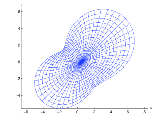
Figure 1: Starlike region with $\widehat{\rho}$ defined by (13) with $a=5$

It is straightforward to show that $F$ is infinitely differentiable for $\left|x\right|<1$, a well-known result. In particular,

$$\frac{\partial F}{\partial x_{1}}=a_{1}+\sum_{m=1}^{\infty}\left(m+1\right)r^{m}\left[a_{m+1}\cos m\theta+b_{m+1}\sin m\theta\right]$$ (10)

$$\frac{\partial F}{\partial x_{2}}=b_{1}+\sum_{m=1}^{\infty}\left(m+1\right)r^{m}\left[-a_{m+1}\sin m\theta+b_{m+1}\cos m\theta\right]$$ (11)

Depending on the speed of convergence of (8), we have the partial derivatives of $F(x)$ are continuous over $\overline{B}_{2}$. In particular, if we have

$$\sum_{n=1}^{\infty}n\left|a_{n}\right|<\infty,\quad\quad\sum_{n=1}^{\infty}n\left|b_{n}\right|<\infty$$

then $\partial F/\partial x_{1}$ and $\partial F/\partial x_{2}$ are continuous over $\overline{B}_{2}$.

Given a boundary function

$$\varphi(\theta)=\left(\varphi_{1}\left(\theta\right),\varphi_{2}\left(\theta\right)\right),\quad\quad 0\leq\theta\leq 2\pi,$$ (12)

we can expand each component to all of $B_{2}$ using the above construction in (9), obtaining a function $\Phi$ defined on $B_{d}$ into $\mathbb{R}^{2}$. A similar construction can be used for higher dimensions using an expansion with spherical harmonics. It is unknown whether the mapping $\Phi$ obtained in this way is a one-to-one mapping from $B_{2}$ onto $\Omega$, even if $\Omega$ is convex.

The method can be implemented as follows.

• Truncate the Fourier series for each of the functions $\varphi_{k}\left(\theta\right)$, $k=1,2,$ say to trigonometric polynomials of degree $n$.

• Approximate the Fourier coefficients $\left\{a_{j}\right\}$ and $\left\{b_{j}\right\}$ for the truncated series.

• Define the extensions $\Phi_{k}\left(x\right)$ in analogy with (9).

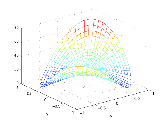
Figure 2: The Jacobian for (13) with $0.905\leq\left|\det\left(D\Phi\left(x\right)\right)\right|\leq 75.314$

Example 1

Choose

$$\rho(\theta)=a+\cos\theta+2\sin 2\theta$$ (13)

with $a$ chosen greater than the maximum of $\left|\cos\theta+2\sin 2\theta\right|$ for $0\leq\theta\leq 2\pi$, approximately 2.2361.  Note that $\rho(\theta)\cos\theta$ and $\rho(\theta)\sin\theta$ are trig polynomials of degree 3. Begin by choosing $a=5$. Choosing  $n=3$, we obtain the graphs in Figures 1 and 2. Figure 1 demonstrates the mapping by showing the images in $\Omega$ of the circles $r=j/p$, $j=0,,\dots,p$ and the azimuthal lines $\theta=\pi j/p$, $j=1,\dots,2p$, $p=15$. For the numerical evaluation of the Fourier coefficients, the trapezoidal rule with $10$ nodes was used. Figure 2 shows $\left|\det\left(D\Phi\left(x\right)\right)\right|$ The figures illustrate that this $\Phi$ is a satisfactory mapping. However, it is possible to improve on this mapping in the sense of reducing the ratio

$$\Lambda\left(\Phi\right)\equiv\frac{\max\limits_{x\in\overline{B}_{2}}\left|\det\left(D\Phi\left(x\right)\right)\right|}{\min\limits_{x\in\overline{B}_{2}}\left|\det\left(D\Phi\left(x\right)\right)\right|}$$ (14)

For the present case, $\Lambda\left(\Phi\right)=100.7$. An iteration method for decreasing the size of $\Lambda\left(\Phi\right)$ is discussed in §4. As a side-note, in the planar graphics throughout this paper we label the axes over the unit disk as $x$ and $y$, and over $\Omega$, we label them as $s$ and $t$.

In contrast to this example, when choosing $a=3$ in (13) the mapping $\Phi$ derived in the same manner is neither one-to-one nor onto. Another method is needed to generate a mapping $\Phi$ which satisfies (13) (2)-(4).

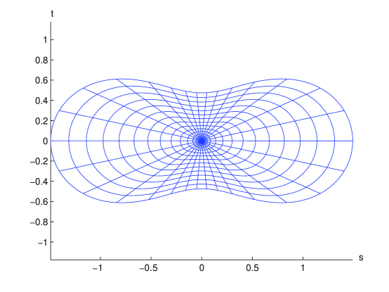
Figure 3: Starlike Cassini region with $\widehat{\rho}$ defined in (17) with $a=1.5$

2.2 Using $C^{\infty}$-modification functions

Let $\left(x,y\right)=\left(r\cos\theta,r\sin\theta\right)$, $0\leq r\leq 1$. As earlier in (5), consider $\Omega$ as star-like with respect to the origin  Introduce the function

$$T(r;\kappa)=\exp\left(\kappa\left(1-\frac{1}{r}\right)\right),\quad\quad 0<r\leq 1$$ (15)

with $\kappa>0$ and $T(0,\kappa)=0$. Define $\Phi$ by

$$s=\Phi\left(x;\kappa,\omega\right)=\left[T\left(r;\kappa\right)\widehat{\rho}\left(\theta\right)+\left(1-T\left(r;\kappa\right)\right)\omega\right]x,\quad\quad x\in B_{2}$$ (16)

with $x=r\left(\cos\theta,\sin\theta\right)$, for $0\leq r\leq 1,\ 0\leq\theta\leq 2\pi$, with some $\omega>0$. This is an attempt to fix the lack of differentiability at (0,0) of the mapping (6)-(7). As $r$ decreases to $0$, we have $\Phi\left(x\right)\approx\omega x$. Thus the Jacobian of $\Phi$ is nonzero around $\left(0,0\right)$. The constants $\kappa,\omega$ are to be used as additional design parameters.

The number $\omega$ should be chosen so as to also ensure the mapping $\Phi$ is 1-1 and onto. Begin by finding a disk centered at $\left(0,0\right)$ that is entirely included in the open set $\Omega$, and say its radius is $\omega_{0},$ or define

$$\omega_{0}=\min_{0\leq\theta\leq 2\pi}\widehat{\rho}\left(\theta\right)$$

Then choose $\omega\in(0,\omega_{0})$. To see this is satisfactory, write

$$\Phi\left(x;\kappa,\omega\right)=f(r)\left(\cos\theta,\sin\theta\right)$$

fixing $\theta\in\left[0,2\pi\right]$. Immediately, $f\left(0\right)=0$, $f\left(1\right)=\widehat{\rho}\left(\theta\right)$. By a straightforward computation,

$$f^{\prime}\left(r\right)=\frac{1}{r}\left\{T\left[\left(\widehat{\rho}-\omega\right)\left(r+1\right)\right]+\omega\right\}$$

where $T=T\left(r;\kappa\right)$ and $\widehat{\rho}=\widehat{\rho}\left(\theta\right)$. The assumption $0<\omega<\omega_{0}$ then implies

$$f^{\prime}\left(r\right)>0,\quad\quad 0<r\leq 1$$

Thus the mapping $f:\left[0,1\right]\rightarrow\left[0,\widehat{\rho}\left(\theta\right)\right]$ is 1-1 and onto, and from this $\Phi:\overline{B}_{2}\rightarrow\overline{\Omega}$ is 1-1 and onto for the definition in (16).

This definition of $\Phi$ satisfies (2)-(4), but often leads to a large value for the ratio $\Lambda\left(\Phi\right)$ of (14). It can be used as an initial choice for a $\Phi$ that can be improved by the iteration method defined in §4.

Example 2

Consider the starlike region with

$$\widehat{\rho}\left(\theta\right)=\sqrt{\cos\left(2\theta\right)+\sqrt{a-\sin^{2}\left(2\theta\right)}}$$ (17)

with $a>1$. The region $\Omega$ is called an ‘ovals of Cassini’. We give an example with $a=1.5$, $\left(\kappa,\omega\right)=\left(1.0,0.5\right)$. Figure 3 is the analog of Figure 1. For the Jacobian,

$$\min_{r\leq 1}D\Phi(x,y) =0.0625\vskip 3.0pt plus 1.0pt minus 1.0pt$$

$$\max_{r\leq 1}D\Phi(x,y) =4.0766$$

The ratio $\Lambda\left(\Phi\right)=65.2$ is large and can be made smaller; see Example 14.

A variation to (16) begins by finding a  closed disk about the origin that is contained wholly in the interior of $\Omega$. Say the closed disk is of radius $\delta,$ $0<\delta<1$. Then define

$$\begin{array}[c]{l}\Phi\left(x;\kappa,\omega\right)\vskip 3.0pt plus 1.0pt minus 1.0pt\\ \quad=\left\{\begin{array}[c]{ll}x,&0\leq r\leq\delta\vskip 6.0pt plus 2.0pt minus 2.0pt\\ \left[T\left(\dfrac{r-\delta}{1-\delta},\kappa\right)\rho\left(\theta\right)+\left(1-T\left(\dfrac{r-\delta}{1-\delta},\kappa\right)\right)\right]x,&\delta<r\leq 1,\end{array}\right.\end{array}$$ (18)

where $x=r\left(\cos\theta,\sin\theta\right)$. Then the Jacobian $D\Phi$ around the origin is simply the identity matrix, and this ensures that $\det D\Phi(x)\neq 0$ for $x\in\overline{B}_{d}$. Experimentation is recommended on the use of either (16) or (18), including how to choose $\kappa$, $\omega$, and $\delta$.

The methods of this section generalize easily to the determination of an extension $\Phi:B_{3}\underset{onto}{\overset{1-1}{\longrightarrow}}\Omega$ for the given boundary mapping

$$\varphi:\partial B_{3}\underset{onto}{\overset{1-1}{\longrightarrow}}\partial\Omega$$

Examples of such are illustrated later in §5.

3 An integration-based mapping formula

Begin by considering a point $P=r(\cos\alpha,\sin\alpha)\in B_{2}$, $r\in[0,1)$, $\alpha\in[0,2\pi)$. Given an angle $\alpha\leq\theta<\pi+\alpha$, draw a line $L$ through $P$ at an angle of $\theta$ with respect to the positive $x_{1}$-axis. Let $P_{+}(\theta)$ and $P_{-}(\theta)$ denote the intersection of this line with the unit disk. These points will have the form

$$\begin{array}[c]{c}P_{+}\left(\theta\right)=P+r_{+}\left(\theta\right)\boldsymbol{\eta},\\ P_{-}\left(\theta\right)=P-r_{-}\left(\theta\right)\boldsymbol{\eta}.\end{array}$$ (19)

with

$$\boldsymbol{\eta}=\left(\cos\theta,\sin\theta\right),\quad\quad\alpha\leq\theta<\pi+\alpha.$$ (20)

We choose $r_{+}\left(\theta\right)$ and $r_{-}\left(\theta\right)$ to be such that

$$\left|P_{+}(\theta)\right|=\left|P+r_{+}\left(\theta\right)\boldsymbol{\eta}\right|=1,\quad\quad\left|P_{-}(\theta)\right|=\left|P-r_{-}\left(\theta\right)\boldsymbol{\eta}\right|=1$$

and

$$\left|r_{+}\left(\theta\right)\right|=\left|P-P_{+}(\theta)\right|,\quad\left|r_{-}\left(\theta\right)\right|=\left|P-P_{-}(\theta)\right|.$$

Define

$$\varphi_{\ast}\left(\theta\right)=\varphi\left(P_{+}\left(\theta\right)\right)-r_{+}(\theta)\frac{\varphi\left(P_{+}\left(\theta\right)\right)-\varphi\left(P_{-}\left(\theta\right)\right)}{r_{+}(\theta)+r_{-}(\theta)}$$ (21)

using linear interpolation along the line $L$. Here and in the following we always identify the function $\varphi$ on the boundary of the unit disk with a $2\pi$ periodic function on the real number line.  Then define

$$\Phi\left(P\right)=\frac{1}{\pi}\int_{\alpha}^{\alpha+\pi}\varphi_{\ast}\left(\theta\right)\,d\theta$$ (22)

We study the construction and properties of $\Phi$ in the following two sections.

3.1 Constructing $\Phi$

The most important construction is the calculation of $P_{+}\left(\theta\right)$ and $P_{-}\left(\theta\right)$. We want to find two points $\boldsymbol{\gamma}$  that are the intersection of $\partial B_{2}$ and the straight line $L$ through $P$ in the direction $\boldsymbol{\eta}$, $\left|\boldsymbol{\eta}\right|=1$.  Since $P\in\operatorname*{int}\left(B_{2}\right)$, we have $\left|P\right|<1$. We want to find

$$\boldsymbol{\gamma}=P+r\boldsymbol{\eta},\quad\quad\left|\boldsymbol{\gamma}\right|=1$$

with $\boldsymbol{\eta}$ denoting the direction from $P$ as noted earlier. With the assumption (20) on  $\boldsymbol{\eta}$, we have

$$\begin{array}[c]{cl}0\leq P\cdot\boldsymbol{\eta}\leq\left|P\right|,&\alpha\leq\theta\leq\alpha+\frac{1}{2}\pi\vskip 3.0pt plus 1.0pt minus 1.0pt\\ 0\leq-P\cdot\boldsymbol{\eta}\leq\left|P\right|,&\alpha+\frac{1}{2}\pi\leq\theta\leq\alpha+\pi\end{array}$$

Using $\boldsymbol{\gamma}\cdot\boldsymbol{\gamma}=1$,

$$\left|P+r\boldsymbol{\eta}\right|^{2}=P\cdot P+2rP\cdot\boldsymbol{\eta}+r^{2}=1$$

$$r^{2}+2rP\cdot\boldsymbol{\eta}+\underset{<0}{\underbrace{P\cdot P-1}}=0$$

which implies the roots are real and nonzero. Thus the formula

$$r =-\boldsymbol{\eta}\cdot P\pm\sqrt{\left(P\cdot\boldsymbol{\eta}\right)^{2}+1-P\cdot P}$$

$$=r\cos(\theta-\alpha)\pm\sqrt{1-r^{2}\sin^{2}(\theta-\alpha)}$$

defines two real roots. Here we see that

$$\left|P\cdot\boldsymbol{\eta}\right|\leq\left|P\right|$$

So

$$r_{-} =P\cdot\boldsymbol{\eta}+\sqrt{\left(P\cdot\boldsymbol{\eta}\right)^{2}+1-P\cdot P}$$

$$=r\cos(\theta-\alpha)+\sqrt{1-r^{2}\sin^{2}(\theta-\alpha)}$$

$$r_{+} =-P\cdot\boldsymbol{\eta}+\sqrt{\left(P\cdot\boldsymbol{\eta}\right)^{2}+1-P\cdot P}$$

$$=-r\cos(\theta-\alpha)+\sqrt{1-r^{2}\sin^{2}(\theta-\alpha)}$$

It is immediate that

$$r_{-}+r_{+} =2\sqrt{\left(P\cdot\boldsymbol{\eta}\right)^{2}+1-P\cdot P}$$

$$=2\sqrt{1-r^{2}\sin^{2}(\theta-\alpha)}$$

and therefore the denominator in the formula (21) for $\varphi_{\ast}\left(\theta\right)$ is zero if and only if  $\left|P\right|=1$ and $P\perp\boldsymbol{\eta}$, a case not allowed in our construction.

Using $r_{-}$ and $r_{+}$ in (19), we can construct $\varphi_{\ast}\left(\theta\right)$ using (21), and this is then used in obtaining the mapping $\Phi\left(P\right)$ of (22). This formula is approximated using numerical integration with the trapezoidal rule. We illustrate this later in the section.

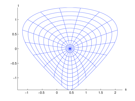
Figure 4: The mapping $\Phi$ for boundary (29) with $a=0.9$

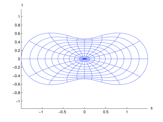
Figure 5: The mapping $\Phi$ for boundary (17) with $a=1.5$

To further simplify the analysis of the mapping $\Phi$ of (22), we assume for a moment that $\alpha=0$, so the point $P$ is located on the positive x–axis. Our next goal is to determine the respective angles between $P_{+}(\theta)$ and $P_{-}(\theta)$ and the positive x-axis. We denote these angles by $\psi^{+}$ and $\psi^{-}$, respectively. Using the law of cosines in the triangle given by the origin, $P$, and $P^{+}$ we obtain

$$(r_{+})^{2} =r^{2}+1-2r\cos(\psi^{+})$$

$$2r\cos(\psi^{+}) =r^{2}+1-(r_{+})^{2}$$

$$=r^{2}+1-\left(-r\cos(\theta)+\sqrt{1-r^{2}\sin^{2}\theta}\right)^{2}$$

$$=2r^{2}\sin^{2}\theta+2r\cos(\theta)\sqrt{1-r^{2}\sin^{2}\theta}$$

which implies

$$\psi_{+}=\psi_{+}(r,\theta)=\arccos\left(r\sin^{2}\theta+\cos(\theta)\sqrt{1-r^{2}\sin^{2}\theta}\right)$$ (23)

where we use the function $\arccos:[-1,1]\mapsto[0,\pi]$. Similarly we get

$$\psi_{-}\equiv\psi_{-}(r,\theta)=\widetilde{\arccos}\left(r\sin^{2}\theta-\cos(\theta)\sqrt{1-r^{2}\sin^{2}\theta}\right)$$ (24)

where we use the function $\widetilde{\arccos}:[-1,1]\mapsto[\pi,2\pi]$,

$$\widetilde{\arccos}(x)=2\pi-\arccos(x)$$

Using the functions $\psi_{-}$ and $\psi_{+}$ we can rewrite $\varphi_{\ast}(\theta)$, see (21), in the following way:

$$\varphi_{\ast}(r,\theta) =\frac{1}{2}\left(1+\frac{r\cos(\theta)}{\sqrt{1-r^{2}\sin^{2}\theta}}\right)\varphi(\psi_{+}(r,\theta))$$

$$+\frac{1}{2}\left(1-\frac{r\cos(\theta)}{\sqrt{1-r^{2}\sin^{2}\theta}}\right)\varphi(\psi_{-}(r,\theta))$$

This allows us to write formula (22) more explicitly in the following way:

$$\Phi(P) =\frac{1}{2\pi}{\displaystyle\int_{0}^{\pi}}\left(1+\frac{r\cos(\theta)}{\sqrt{1-r^{2}\sin^{2}\theta}}\right)\varphi(\psi_{+}(r,\theta))d\theta$$

$$+\frac{1}{2\pi}{\displaystyle\int_{0}^{\pi}}\left(1-\frac{r\cos(\theta)}{\sqrt{1-r^{2}\sin^{2}\theta}}\right)\varphi(\psi_{-}(r,\theta))d\theta$$

$$=\frac{1}{2\pi}{\displaystyle\int_{0}^{\pi}}\left(1+\frac{r\cos(\theta)}{\sqrt{1-r^{2}\sin^{2}\theta}}\right)\varphi(\psi_{+}(r,\theta))d\theta$$

$$+\frac{1}{2\pi}{\displaystyle\int_{\pi}^{2\pi}}\left(1-\frac{r\cos(\theta-\pi)}{\sqrt{1-r^{2}\sin^{2}(\theta-\pi)}}\right)\varphi(\psi_{-}(r,\theta-\pi))d\theta$$

$$=\frac{1}{2\pi}{\displaystyle\int_{0}^{\pi}}\left(1+\frac{r\cos(\theta)}{\sqrt{1-r^{2}\sin^{2}\theta}}\right)\varphi(\psi_{+}(r,\theta))d\theta$$

$$+\frac{1}{2\pi}{\displaystyle\int_{\pi}^{2\pi}}\left(1+\frac{r\cos(\theta)}{\sqrt{1-r^{2}\sin^{2}\theta}}\right)\varphi(\psi_{-}(r,\theta-\pi))d\theta$$

$$=\frac{1}{2\pi}{\displaystyle\int_{0}^{2\pi}}\left(1+\frac{r\cos(\theta)}{\sqrt{1-r^{2}\sin^{2}\theta}}\right)\varphi(\psi_{\ast}(r,\theta))d\theta$$ (25)

Here we used the variable transformation $\theta\mapsto\pi+\theta$ for the second equality and the new definition

$$\psi_{\ast}(r,\theta):=\left\{\begin{array}[c]{cl}\psi_{+}(r,\theta),&0\leq\theta\leq\pi\vskip 3.0pt plus 1.0pt minus 1.0pt\\ \psi_{-}(r,\theta-\pi),&\pi<\theta\leq 2\pi\end{array}\right.$$ (26)

where the functions $\psi_{-}$ and $\psi_{+}$ are defined in (23) and (24). We remark, that the function $\psi_{\ast}:[0,1)\times[0,2\pi]\mapsto[0,2\pi]$ is a continuous function which follows from its geometric construction. We further define

$$k(r,\theta):=1+\frac{r\cos(\theta)}{\sqrt{1-r^{2}\sin^{2}\theta}}$$ (27)

a $2\pi$ periodic continuous function on $[0,1)\times[0,2\pi]$. If we now go back to the general case $P=r(\cos(\alpha),\sin(\alpha))$, $\alpha\in[0,2\pi)$, we can rotate the given boundary function $\varphi$ and obtain

$$(\mathcal{E}\varphi)(P)\equiv\Phi(P)=\frac{1}{2\pi}\int_{0}^{2\pi}k(r,\theta)\varphi(\psi_{\ast}(r,\theta)+\alpha)d\theta$$ (28)

Before we study the properties of the extension operator $\mathcal{E}$, we present two numerical examples.

To obtain $\Phi\left(P\right)$, we apply the trapezoidal rule to approximate the integral in (28) or (22). The number of integration nodes should be chosen sufficiently large, although experimentation is needed to determine an adequate choice.

Example 3

Consider

$$\varphi\left(\cos\theta,\sin\theta\right)=\left(\cos\theta-\sin\theta+a\cos^{2}\theta,\cos\theta+\sin\theta\right),\quad 0\leq\theta\leq 2\pi$$ (29)

with $0<a<1$. We choose $a=0.9$ and apply the above with $n=100$ subdivisions for the trapezoidal rule to evaluate (22). Figure 4 shows the mapping $\Phi$, done in the same manner as earlier with Figures 1 and 3.

Example 4

We consider again the ovals of Cassini region with boundary given in (17) with $a=1.5$. The mapping (22) is illustrated in Figure 5. However, for $a$ somewhat closer to 1, this integration formula (22) no longer produces a satisfactory $\Phi$.

3.2 Properties of $\mathcal{E}\varphi$

To study the properties of the extension operator $\mathcal{E}$, see (28), we have to study the behavior of the functions $\psi_{\ast}$ and $k$, see (26) and (27), at the boundary $r=1$. We start with the function $\psi_{\ast}$ and define the values of this function for $r=1$ first:

$$\psi_{\ast}(1,\theta):=\left\{\begin{array}[c]{cl}0,&0\leq\theta\leq\frac{1}{2}\pi\vskip 3.0pt plus 1.0pt minus 1.0pt\\ 2\theta-\pi,&\frac{1}{2}\pi\leq\theta\leq\frac{3}{2}\pi\vskip 3.0pt plus 1.0pt minus 1.0pt\\ 2\pi,&\frac{3}{2}\pi\leq\theta\leq 2\pi\end{array}\right.$$ (30)

Because of

$$\lim_{r\rightarrow 1}1-r^{2}=0$$

and the boundedness of the sine function, the limit

$$\lim_{r\rightarrow 1}1-r^{2}\sin^{2}(\theta)=1-\sin^{2}(\theta),$$

is uniform for $\theta\in\left[0,\frac{1}{2}\pi\right]$. The uniform continuity of the square root function implies that

$$\lim_{r\rightarrow 1^{-}}\left(\cos(\theta)\sqrt{1-r^{2}\sin^{2}\theta}\right) =\cos(\theta)\sqrt{1-\sin^{2}\theta}$$

$$=\cos^{2}\theta$$

uniformly for $\theta\in\left[0,\frac{1}{2}\pi\right]$. Together with similar arguments for the function $r$ we get

$$\lim_{r\rightarrow 1^{-}}\left(r\sin^{2}\theta+\cos(\theta)\sqrt{1-r^{2}\sin^{2}\theta}\right)=\sin^{2}\theta+\cos^{2}\theta=1$$

uniformly in $\theta$. Finally we use the uniform continuity of $\arccos(\cdot)$ to conclude that

$$\lim_{r\rightarrow 1^{-}}\psi_{\ast}(r,\theta) =\lim_{r\rightarrow 1^{-}}\arccos\left(r\sin^{2}\theta+\cos(\theta)\sqrt{1-r^{2}\sin^{2}\theta}\right)$$

$$=\arccos(1)$$

$$=0\>=\psi_{\ast}(1,\theta)$$

converges uniformly on $\left[0,\frac{1}{2}\pi\right]$. Because

$$\sqrt{1-\sin^{2}(\theta)}=-\cos(\theta),\quad\quad\theta\in\left[\tfrac{1}{2}\pi,\pi\right],$$

we see in a similar way that

$$\lim_{r\rightarrow 1^{-}}\psi_{\ast}(r,\theta) =\lim_{r\rightarrow 1^{-}}\arccos\left(r\sin^{2}\theta+\cos(\theta)\sqrt{1-r^{2}\sin^{2}\theta}\right)$$

$$=\arccos(\sin^{2}\theta+\cos(\theta)(-\cos(\theta)))$$

$$=\arccos(-\cos(2\theta))$$

$$=\arccos(\cos(2\theta-\pi))$$

$$=2\theta-\pi$$

$$=\psi_{\ast}(1,\theta)$$

uniformly for $\theta\in\left[\frac{1}{2}\pi,\pi\right]$. Similar arguments apply for $\theta\in[\pi,2\pi]$ and we finally conclude that $\psi_{\ast}(r,\theta)$ converges uniformly to $\psi_{\ast}(1,\theta)$ as $r$ approaches $1$. This proves the next lemma.

Lemma 5

The function $\psi_{\ast}$, defined by (26) and (30), is continuous on $[0,1]\times[0,2\pi]$.

We remark that continuity on a closed interval implies uniform continuity.

Now we turn to the function $k$ defined in (27). Here we define $k$ for the value $r=1$ in the following way

$$k(1,\theta):=\left\{\begin{array}[c]{rl}2,&0\leq\theta<\frac{1}{2}\pi\vskip 3.0pt plus 1.0pt minus 1.0pt\\ 0,&\frac{1}{2}\pi\leq\theta\leq\frac{3}{2}\pi\vskip 3.0pt plus 1.0pt minus 1.0pt\\ 2,&\frac{3}{2}\pi<\theta\leq 2\pi\end{array}\right.$$ (31)

Obviously $k(1,\cdot)$ cannot be the uniform limit of $k(r,\cdot)$ as $r$ approaches $1$, but the following lemma holds.

Lemma 6

The function $k:[0,1]\times[0,2\pi]\mapsto[0,2]$, defined by (27) and (31), is bounded; and for every $\delta>0,$ the function $k(r,\theta)$ approaches $k(1,\theta)$ uniformly on $I_{\delta}$ as $r$ approaches $1$. Here

$$I_{\delta}:=[0,2\pi]\setminus\left\{\left(\tfrac{1}{2}\pi-\delta,\tfrac{1}{2}\pi+\delta\right)\cup\left(\tfrac{3}{2}\pi-\delta,\tfrac{3}{2}\pi+\delta\right)\right\}$$

Proof. That $k$ is bounded by $2$ follows from

$$\sqrt{1-r^{2}\sin^{2}\theta}\geq\sqrt{1-\sin^{2}\theta}=|\cos(\theta)|$$

and the fact that $r\in[0,1]$. The function $1/\sqrt{z}$ is uniformly continuous on $\varepsilon\leq z\leq 1$ for every $\varepsilon>0$. From the proof of Lemma 5 we know that

$$\lim_{r\rightarrow 1^{-}}1-r^{2}\sin^{2}\theta=\cos^{2}\theta$$

uniformly for $\theta\in[0,2\pi]$. Together with the uniform continuity of $1/\sqrt{z}$ on $[\cos^{2}(\frac{1}{2}\pi-\delta),1],$ this shows

$$\lim_{r\rightarrow 1^{-}}1+\frac{r\cos(\theta)}{\sqrt{1-r^{2}\sin^{2}\theta}}=1+\frac{\cos(\theta)}{|\cos(\theta)|}$$

uniformly on $I_{\delta}$. Remembering

$$|\cos(\theta)|=\left\{\begin{array}[c]{rl}\cos(\theta),&\theta\in\left[0,\frac{1}{2}\pi\right]\cup\left[\frac{3}{2}\pi,2\pi\right]\vskip 3.0pt plus 1.0pt minus 1.0pt\\ -\cos(\theta),&\theta\in\left[\frac{1}{2}\pi,\frac{3}{2}\pi\right]\end{array}\right.$$

proves the Lemma.   

Motivated by the properties of $\psi_{\ast}$ and $k$ we now prove a more general result for integral operators of the form (28).

Lemma 7

Let $k_{1},k_{2}:[0,1]\times[0,2\pi]\mapsto\mathbb{R}$ be bounded functions which are continuous on $[0,1)\times[0,2\pi]$. Assume there is a finite set $E=\{\theta_{1},\ldots,\theta_{n}\}$ such that

$$\lim_{r\rightarrow 1^{-}}k_{i}(r,\theta)=k_{i}(1,\theta),\quad\quad i=1,2,$$

uniformly on $I_{\delta}:=\{\theta\in[0,2\pi]\mid|\theta-\theta_{j}|\geq\delta,\,j=1,\ldots,n\}$ for every $\delta>0$. Then for a periodic continuous function $\varphi:[0,2\pi]\mapsto\mathbb{R}$ the function

$$\Phi(r,\alpha):=\int_{0}^{2\pi}k_{1}(r,\theta)\varphi(k_{2}(r,\theta)+\alpha)\,d\theta$$

is continuous on $[0,1]\times[0,2\pi]$ and $2\pi$ periodic in $\alpha$.

Remark 8

The above lemma will apply to each component of the function $\mathcal{E}\varphi$ defined in (28) with $k_{1}=k$ and $k_{2}=\psi_{\ast}$ and $E=\{\frac{1}{2}\pi,\frac{3}{2}\pi\}$. This shows the continuity of $\mathcal{E}\varphi$.

Proof. The uniform convergence on $I_{\delta}$, $\delta>0$ arbitrary, shows that $k_{i}(1,\cdot)$, $i=1,2$, are piecewise continuous and bounded functions on $[0,2\pi]$, so all integrals exist. The continuity of $\Phi(r,\alpha)$ on $[0,1)\times[0,2\pi]$ follows easily from the continuity of the functions $k_{i}$, $i=1,2$. The periodicity follows from the periodicity of $\varphi$ and the definition of $\Phi$. So we only need to show the continuity of $\Phi(r,\alpha)$ on $\{1\}\times[0,2\pi]$ for example at $(1,\overline{\alpha})$. Because of the periodicity of $\Phi(r,\cdot)$ and the property $(\mathcal{E}\varphi)(\alpha)=(\mathcal{E}\varphi_{\alpha})(0)$, where $\varphi_{\alpha}(\theta)=\varphi(\alpha+\theta)$ we only need to prove the continuity for one value of $\overline{\alpha}$, for example $\alpha=\pi$. We estimate

$$|\Phi(r,\alpha)-\Phi(1,\pi)| =\left|\int_{0}^{2\pi}k_{1}(r,\theta)\varphi(k_{2}(r,\theta)+\alpha)-k_{1}(1,\theta)\varphi(k_{2}(1,\theta)+\pi)\,d\theta\right|$$

$$\leq\left|\int_{0}^{2\pi}k_{1}(r,\theta)(\varphi(k_{2}(r,\theta)+\alpha)-\varphi(k_{2}(1,\theta)+\pi))\,d\theta\right|$$

$$+\left|\int_{0}^{2\pi}(k_{1}(r,\theta)-k_{1}(1,\theta))\varphi(k_{2}(1,\theta)+\pi))\,d\theta\right|$$

Now we know that $k_{1},k_{2},$ and $\varphi$ are bounded functions, for example

$$|k_{1}(r,\theta)|,|k_{1}(r,\theta)|,|\varphi(\theta)|\leq M,\quad\quad M>0$$

for all $(r,\theta)\in[0,1]\times[0,2\pi]$. So we only have to show

$$\lim_{r\rightarrow 1}\int_{0}^{2\pi}|\varphi(k_{2}(r,\theta)+\alpha)-\varphi(k_{2}(1,\theta)+\pi)|\,d\theta=0$$ (32)

and

$$\lim_{r\rightarrow 1}\int_{0}^{2\pi}|k_{1}(r,\theta)-k_{1}(1,\theta)|\,d\theta=0$$ (33)

We start with the first limit. Given an $\varepsilon>0$ we choose $\delta>0$ small enough such that

$$\int_{[0,2\pi]\setminus I_{\delta}}2M\;d\theta=\frac{\varepsilon}{2}$$ (34)

Now we observe that $\varphi$ is uniformly continuous on $\mathbb{R}$ because it is continuous and periodic. So there is a $\omega>0$ such that

$$|\varphi(x)-\varphi(y)|\leq\frac{\varepsilon}{4\pi}$$ (35)

if $|x-y|\leq\omega$. We also know that $k_{2}(r,\cdot)$ converges uniformly on $I_{\delta}$ to $k_{2}(1,\cdot)$, so there is a $r_{0}\in(0,1)$, such that

$$|k_{2}(r,\theta)-k_{2}(1,\theta)|\leq\frac{\omega}{2}$$

for all $r\geq r_{0}$ and $\theta\in I_{\delta}$. If furthermore $|\alpha-\pi|\leq\omega/2$, we conclude that

$$|(k_{2}(r,\theta)+\alpha)-(k_{2}(1,\theta)+\pi)| \leq|k_{2}(r,\theta)-k_{1}(1,\theta)|+|\alpha-\pi|$$

$$\leq\omega$$

which by (35) implies

$$|\varphi(k_{2}(r,\theta)+\alpha)-\varphi(k_{2}(1,\theta)+\pi)|\leq\frac{\varepsilon}{4\pi}$$ (36)

for all $(r,\alpha)\in[r_{0},1]\times[\pi-\omega/2,\pi+\omega/2]$ and $\theta\in I_{\delta}$. Combining (34) and (36) we can estimate

$$\int_{0}^{2\pi}|\varphi(k_{2}(r,\theta)+\alpha)-\varphi(k_{2}(1,\theta)+\pi)|\,d\theta$$

$$\leq\int_{[0,2\pi]\setminus I_{\delta}}|\varphi(k_{2}(r,\theta)+\alpha)-\varphi(k_{2}(1,\theta)+\pi)|\,d\theta$$

$$+\int_{I_{\delta}}|\varphi(k_{2}(r,\theta)+\alpha)-\varphi(k_{2}(1,\theta)+\pi)|\,d\theta$$

$$\leq\int_{[0,2\pi]\setminus I_{\delta}}2M\;d\theta+\int_{I_{\delta}}\frac{\varepsilon}{4\pi}\,d\theta$$

$$\leq\frac{\varepsilon}{2}+2\pi\cdot\frac{\varepsilon}{4\pi}=\varepsilon$$

for all $(r,\alpha)\in[r_{0},1]\times[\pi-\omega/2,\pi+\omega/2]$,which proves (32).

To prove (33) we again choose an arbitrary $\varepsilon>0$ and choose $\delta>0$ such that (34) is true. Now the uniform convergence of $k_{1}(r,\cdot)$ to $k_{1}(1,\cdot)$ on $I_{\delta}$ proves the existence of a $r_{1}\in(0,1)$ such that

$$|k_{1}(r,\theta)-k_{1}(1,\theta)|\leq\frac{\varepsilon}{4\pi}$$ (37)

for all $(r,\theta)\in[r_{1},1]\times I_{\delta}$. Using (34) and (37) we estimate

$$\int_{0}^{2\pi}|k_{1}(r,\theta)-k_{1}(1,\theta)|\;d\theta =\int_{[0,2\pi]\setminus I_{\delta}}|k_{1}(r,\theta)-k_{1}(1,\theta)|\,d\theta$$

$$+\int_{I_{\delta}}|k_{1}(r,\theta)-k_{1}(1,\theta)|\,d\theta$$

$$\leq\int_{[0,2\pi]\setminus I_{\delta}}2M\,d\theta+\int_{I_{\delta}}\frac{\varepsilon}{4\pi}\,d\theta$$

$$\leq\frac{\varepsilon}{2}+2\pi\cdot\frac{\varepsilon}{4\pi}=\varepsilon$$

for all $r\in[r_{1},1]$. This proves (33).   

Now we state the results about the extension operator $\mathcal{E}$.

Theorem 9

Let $\varphi:\partial B_{2}\mapsto\mathbb{R}^{2}$, be a continuous function, then $\Phi(P)=(\mathcal{E}\varphi)(r,\alpha)$, $P\in\overline{B_{2}}$, see (28), is continuous function on $\overline{B_{2}}$ and

$$\Phi|_{\partial B_{2}} =\varphi$$ (38)

Proof. In Lemma 5 and Lemma 6 we have shown that the functions $k$ and $\psi_{\ast}$ in (28) satisfy the assumptions of Lemma 7. So the continuity of $\Phi(P)$ follows from Lemma 7. For $P\in\partial B_{2}$ the polar coordinates of $P$ are given by $(r,\alpha)=(1,\alpha)$, $\alpha\in[0,2\pi]$, so we get with (30) and (31)

$$\Phi(P) =\frac{1}{2\pi}\int_{0}^{2\pi}k(1,\theta)\varphi(\psi_{\ast}(1,\theta)+\alpha)\,d\theta$$

$$=\frac{1}{2\pi}\left(\int_{0}^{\pi/2}2\varphi(0+\alpha)\;d\theta+\int_{3\pi/2}^{2\pi}2\varphi(2\pi+\alpha)\,d\theta\right)$$

$$=\frac{1}{2\pi}(\pi\varphi(\alpha)+\pi\varphi(2\pi+\alpha))$$

$$=\varphi(\alpha)=\varphi(P)$$

because of the $2\pi$ periodicity of $\varphi$.   

Corollary 10

Let $\Omega\subset\mathbb{R}^{2}$ be a domain with boundary $\partial\Omega$ and $\varphi:\partial B_{2}\mapsto\partial\Omega$ be a continuous parametrization of the boundary. Then the function $\mathcal{E}\varphi$, defined in (28), maps $\overline{B_{2}}$ onto $\overline{\Omega}$.

Proof. Theorem 9 implies that $\mathcal{E}\varphi:\overline{B_{2}}\mapsto\mathbb{R}^{2}$ is continuous and that $(\mathcal{E}\varphi)(\partial B_{2})=\partial\Omega$. We assume that the parametrization $\varphi$ moves along the boundary of $\Omega$ in the positive direction. For $y\in\Omega$ we then have

$$\deg(\mathcal{E}\varphi,y)=1$$

where $\deg$ is the mapping degree; see [10, Chapter 12]. But this implies that there is at least one $x\in B_{2}$ such that $(\mathcal{E}\varphi)(x)=y$.   

Theorem 11

Let $\Omega\subset\mathbb{R}^{2}$ be a convex domain with boundary $\partial\Omega$ and $\varphi:\partial B_{2}\mapsto\partial\Omega$ be a continuous parametrization of the boundary. Then $(\mathcal{E}\varphi)(B_{2})\subset\overline{\Omega}$.

Proof. We have to show $(\mathcal{E}\varphi)(P)\in\overline{\Omega}$ for every $P\in B_{2}$. We use the first equation in formula (25)

$$\Phi(P) =\frac{1}{2\pi}\int_{0}^{\pi}\left(1+\frac{r\cos(\theta)}{\sqrt{1-r^{2}\sin^{2}(\theta)}}\right)\varphi(\psi_{+}(r,\theta))$$

$$+\left(1-\frac{r\cos(\theta)}{\sqrt{1-r^{2}\sin^{2}(\theta)}}\right)\varphi(\psi_{-}(r,\theta))\,d\theta$$

$$=\lim_{N\rightarrow\infty}\frac{1}{N}\sum_{j=0}^{N}\left(\frac{1}{2}+\frac{r\cos(\theta_{j})}{2\sqrt{1-r^{2}\sin^{2}(\theta_{j})}}\right)\varphi(\psi_{+}(r,\theta_{j}))$$

$$+\left(\frac{1}{2}-\frac{r\cos(\theta_{j})}{2\sqrt{1-r^{2}\sin^{2}(\theta_{j})}}\right)\varphi(\psi_{-}(r,\theta_{j}))$$

where $\theta_{j}=\pi j/N$ and we further assumed again that $P$ is on the positive real axis to simplify the notation. Here we have used the fact that the integral is the limit of Riemann sums. Each term of the sum is a convex combination of two elements of $\overline{\Omega}$ and therefore in $\overline{\Omega}$. But the sum itself is a convex combination, so the sum is an element of $\overline{\Omega}$. Finally $\overline{\Omega}$ is closed, so $\Phi(P)\in\overline{\Omega}$.   

The two last results imply that for a convex domain $\Omega$ we get $(\mathcal{E}\varphi)(\overline{B_{2}})=\overline{\Omega}$, but there is still the possibility that $\mathcal{E}(\varphi)$ is not injective. Our numerical examples seem to indicate that the function is injective for convex $\Omega$, but we have no proof. For non-convex regions, it works for some but not others. It is another option in a toolkit of methods for producing the mapping $\Phi$.

The integration-based formula (22) can be extended to three dimensions. Given

$$\varphi:\partial B_{3}\underset{onto}{\overset{1-1}{\longrightarrow}}\partial\Omega,$$

define the interpolation formula $\varphi_{\ast}\left(\theta,\omega\right)$ as before in (21), with $\left(\theta,\omega\right)$ the spherical coordinates of a direction vector $\boldsymbol{\eta}$ through a given point $P\in B_{3}$. Then define

$$\Phi\left(P\right)=\frac{1}{2\pi}\int_{0}^{2\pi}\int_{0}^{\pi/2}\varphi_{\ast}\left(\theta,\omega\right)\sin\omega\,d\omega\,d\theta$$ (39)

A proof of the generalization of Corollary 10 can be given along the same line as given above for the disk $B_{2}$.

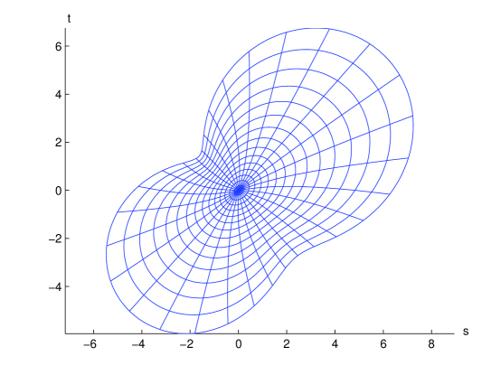
Figure 6: The initial mapping $\widetilde{\Phi}$ for Example 12 with $a=5$,  based on (16)

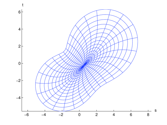
Figure 7: The mapping $\Phi$ for Example 12 with $a=5$, obtained using iteration

4 Iteration methods

Some of the methods discussed in §2 lead to a mapping $\Phi$ in which $\det\left(D\Phi\left(x\right)\right)$ has a large variation as $x$ ranges over the unit ball $B_{d}$, especially those methods based on using using the $C^{\infty}$-function $T\left(r,\kappa\right)$ of (16).  We seek a way to improve on such a mapping, to obtain a mapping in which $\det\left(D\Phi\left(x\right)\right)$ has a smaller variation over $B_{d}$. We continue to look at only the planar problem, while keeping in mind the need for a method that generalizes to higher dimensions. In this section we introduce an iteration method to produce a mapping $\Phi$ with each component a multivariate polynomial over $B_{2}$.

Assume we have an initial guess for our mapping, in the form of a polynomial of degree $n$,

$$\Phi_{n}^{(0)}\left(x\right)\equiv\sum_{j=1}^{N_{n}}\alpha_{j}^{(0)}\psi_{j}(x),\quad\quad x\in B_{2}$$ (40)

We want to calculate an ‘improved’ value for $\Phi_{n}^{(0)}$, call it $\Phi_{n}$.

The coefficients $\alpha_{j}^{(0)}\in\mathbb{R}^{2}$. The functions $\left\{\psi_{1},\dots,\psi_{N_{n}}\right\}$ are chosen to be a basis for $\Pi_{n}$, the polynomials of degree $\leq n$. and we require them to be orthonormal with respect to the inner product $\left(\cdot,\cdot\right)$ associated with $L^{2}\left(B_{2}\right)$. Note that $N_{n}=\dim\left(\Pi_{n}\right)=\frac{1}{2}\left(n+1\right)\left(n+2\right)$. As basis functions $\left\{\psi_{j}\right\}$ in our numerical examples, we use the ‘ridge polynomials’ of Logan and Shepp [6], an easy basis to define and calculate; also see [3, §4.3.1].

We use an iterative procedure to seek an approximation

$$\Phi_{n}\left(x\right)=\sum_{j=1}^{N_{n}}\alpha_{n,j}\psi_{j}(x)$$ (41)

of degree $n$ that is an improvement in some sense on $\Phi_{n}^{(0)}$.  The degree $n$ used in defining $\Phi_{n}^{\left(0\right)}$, and also in defining our improved value $\Phi_{n}$, will need to be sufficiently large; and usually, $n$ must be determined experimentally.

The coefficients $\left\{\alpha_{j}^{(0)}\right\}$ are normally generated by numerical integration of the Fourier coefficients $\left\{\alpha_{j}^{(0)}\right\}$,

$$\alpha_{j}^{(0)}=\left(\widetilde{\Phi},\psi_{j}\right),$$ (42)

where $\widetilde{\Phi}$ is generated by one of the methods discussed in §§2,3. The quadrature used is

$$\int_{B_{2}}g(x,y)\,dx\,dy\approx\frac{2\pi}{2p+1}\sum_{l=0}^{p}\sum_{m=0}^{2p}\omega_{l}r_{l}\widehat{g}\left(r_{l},\frac{2\pi\,m}{2p+1}\right)$$ (43)

where $\widehat{g}\left(r,\theta\right)\equiv g\left(r\cos\theta,r\sin\theta\right)$. Here the numbers $\left\{\omega_{l}\right\}$ are the weights of the $\left(p+1\right)$-point Gauss-Legendre quadrature formula on $[0,1]$, and the nodes $\left\{r_{l}\right\}$ are the corresponding zeros the the degree $p+1$ Legendre polynomial on $\left[0,1\right]$.  This formula is exact if $g$ is a polynomial of degree $\leq 2p+1$; see [8, §2.6].

We need to require that our mapping will agree with $\varphi$ on $S^{1}$, at least approximately.  To this end, choose a formula $q_{n}$ for the number of points on $S^{1}$ at which to match $\Phi_{n}$ with the function $\varphi$ and then choose $\left\{z_{1},\dots,z_{q_{n}}\right\}$ on $S^{1}$. Require $\Phi_{n}$ to satisfy

$$\Phi_{n}\left(z_{j}\right)=\varphi\left(z_{j}\right),\quad\quad j=1,\dots,q_{n}$$ (44)

which imposes implicitly $q_{n}$ conditions on the coefficients $\left\{\alpha_{n,j}\right\}$. If $\varphi$ is a trigonometric polynomial of degree $m$, and if $n\geq m$ with $q_{n}=2n+1$, then (44) will imply that $\left.\Phi_{n}\right|_{S^{1}}=\varphi$ over $\partial\Omega$. Our numerical examples all use this latter choice of $q_{n}$.

Next, choose a function $\mathcal{F}\left(\alpha\right)$, $\alpha=\left[\alpha_{1},\dots,\alpha_{N}\right]^{\text{T}}$, and seek to calculate $\alpha$ so as to minimize $\mathcal{F}(\alpha)$ subject to the above constraints (44). How should $\mathcal{F}$ be chosen? To date, the most successful choice experimentally has been $\mathcal{F}\left(\alpha\right)=\Lambda\left(\Phi_{n}\right),$ defined earlier in (14).

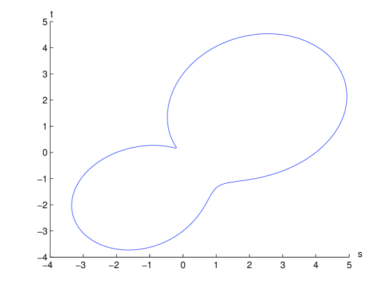
Figure 8: The boundary for the starlike region with $\rho=3+\cos\theta+2\sin 2\theta$

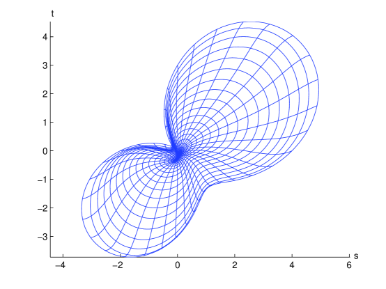
Figure 9: The boundary mapping $\Phi$ for the starlike region
with $\rho=3+\cos\theta+2\sin 2\theta$

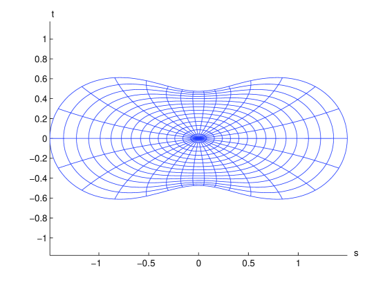
Figure 10: The boundary mapping $\Phi$ for the starlike region with $\rho$ from (17) with $a=1.5$

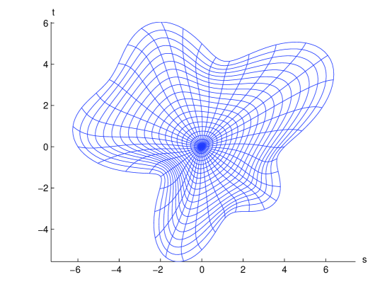
Figure 11: The optimal mapping $\Phi_{7}$ for the starlike region with $\widehat{\rho}\left(\theta\right)=5+\sin\theta+\sin 3\theta-\cos 5\theta$

4.1 The iteration algorithm

Using the constraints (44) leads to the system

$$A\alpha=\mathbf{\varphi},$$ (45)

$$A=\left[\begin{array}[c]{ccc}\psi_{1}(z_{1})&\cdots&\psi_{N}(z_{1})\\ \vdots&&\vdots\\ \psi_{1}(z_{q})&\cdots&\psi_{N}(z_{q})\end{array}\right],\quad\quad\mathbf{\varphi=}\left[\begin{array}[c]{c}\varphi_{1}(z_{1})\\ \vdots\\ \varphi_{1}(z_{q})\end{array}\right]$$

Because $\left.\Phi_{n}\right|_{S^{1}}$ is a trigonometric polynomial of degree $n$, it is a bad idea to have $q_{n}>2n+1$. The maximum row rank of $A$ can be at most $2n+1$. Let $\left\{z_{1},\dots,z_{q}\right\}$ denote $q_{n}$ evenly spaced points on $S^{1}$. We want to minimize $\mathcal{F}\left(\alpha\right)$ subject to the constraints (45).

We turn our constrained minimization problem into an unconstrained problem. Let $A=UCV$ be the singular value decomposition of $A$; $U$ is an orthogonal matrix of order $q$, $V$ is an orthogonal matrix of order $N$, and $C$ is a ‘diagonal matrix’ of order $q\times N$. The constraints (45) can be written as

$$CV\alpha=U^{\text{T}}\mathbf{\varphi}$$ (46)

Introduce a new variable $\beta=V\alpha$, or $\alpha=V^{\text{T}}\beta$. Then $C\beta=U^{\text{T}}\mathbf{\varphi}$ and we can solve explicitly for $\gamma=[\beta_{1},\dots,\beta_{q}]^{\text{T}}$. Implicitly this assumes that $A$ has full rank. Let $\delta=[\beta_{q+1},\dots,\beta_{N}]^{\text{T}}$, $\beta=\left[\gamma^{\text{T}},\delta^{\text{T}}\right]^{\text{T}}$.   Then introduce

$$G\left(\delta\right)=\mathcal{F}\left(\alpha\right)$$ (47)

using $\alpha=V^{\text{T}}\beta$ and the known values of $\gamma$. We use our initial $\left\{\alpha_{j}^{(0)}\right\}$ in (40) to generate the initial value for $\beta$ and thus for $\delta$.

The drawback to this iteration method is the needed storage for the $q\times N$ matrix $A$ and the matrices produced in its singular value decomposition. In the following numerical examples, we minimize $G$ using the Matlab program fminunc for unconstrained minimization problems.

Example 12

Recall Example 1 with $a=5$. Generate an initial mapping $\widetilde{\Phi}$ using (16) with $\kappa=.5$, $\omega=1.0$. Next, generate an initial polynomial (40) of degree $n=3$, using numerical integration of the Fourier coefficients $\left\{\alpha_{j}^{(0)}\right\}$ of (42). We then use the above iteration method to obtain an improved mapping. Figure 6 shows the initial mapping $\widetilde{\Phi}$, and Figure 7 shows the final mapping $\Phi_{n}$ obtained by the iteration method. With the final mapping, we have $\left.\Phi_{n}\right|_{S^{1}}=\varphi$ to double precision rounding accuracy, and

$$\Lambda\left(\Phi\right)=6.21$$

Compare the latter to $\Lambda\left(\Phi\right)=100.7$ for the mapping in Example 1.

Example 13

Consider again the starlike region using (13) of Example 1, but now with $a=3$. The harmonic mapping of §2.1 failed in this case to produce a 1-1 mapping. In fact, the boundary is quite ill-behaved in the neighborhood of $\left(-0.2,0.2\right)$, being almost a corner; see Figure 8. In this case we needed $n=7$, with this smallest sufficient degree determined experimentally. To generate the initial guess $\widetilde{\Phi}$, we used (16) with $\left(\kappa,\omega\right)=\left(0.5,0.1\right)$. For the initial guess, $\Lambda\left(\Phi_{7}^{(0)}\right)\doteq 840.$ We iterated first with the Matlab program fminunc. When it appeared to converge, we used the resulting minimizer as an initial guess with a call to the Matlab routine fminsearch, which is a Nelder-Mead search method. When it converged, its minimizer was used again as an initial guess, returning to a call on fminunc. Figure 9 shows the final mapping $\Phi_{7}$ obtained with this repeated iteration. For the Jacobian matrix, $\Lambda\left(\Phi_{7}\right)\doteq 177.9$, further illustrating the ill-behaviour associated with this boundary. As before, $\left.\Phi\right|_{S^{1}}=\varphi$ to double precision rounding accuracy.

Example 14

Consider again the ovals of Cassini region with boundary given in (17) with $a=1.5$. As our initial mapping $\widetilde{\Phi}$, we use the interpolating integration-based mapping of (22), illustrated in Figure 5. We produce the initial guess for the coefficients $\left\{\alpha_{j}^{(0)}\right\}$ of (42) by using numerical integration. Unlike the preceding three examples, the boundary mapping $\varphi$ is not a trigonometric polynomial, and thus the interpolating conditions of (44) will not force $\left.\Phi_{n}\right|_{S^{1}}$ to equal $\varphi$ over $\partial\Omega$. For that reason, we use a higher degree than with the preceding examples, choosing $n=16$. Figure 10 shows the resulting mapping $\Phi$. With this mapping, $\Lambda\left(\Phi\right)=26.11$. On the boundary,

$$\max_{x\in S^{1}}\left|\Phi\left(x\right)-\varphi\left(x\right)\right|=2.61E-4$$

showing the mapping does not depart far from the region $\overline{\Omega}$.

Example 15

Consider the starlike domain with

$$\widehat{\rho}\left(\theta\right)=5+\sin\theta+\sin 3\theta-\cos 5\theta,\quad\quad 0\leq\theta\leq 2\pi.$$

in (6)-(7). Using the degree $n=7$ and the inital mapping $\widetilde{\Phi}$ based on (16) with $\left(\kappa,\omega\right)=\left(0.2,\,1.4\right)$, we obtained the mapping illustrated in Figure 11. The minimum value obtained was $\Lambda\left(\Phi_{7}\right)\doteq 6.63$. As a side-note of interest, the iteration converged to a value of $\Lambda\left(\Phi\right)$ that varied with the initial choice of $\left(\kappa,\omega\right)$. We have no explanation for this, other than to say that the objective function $\Lambda\left(\Phi\right)$ appears to be ill-behaved in some sense that we do not yet understand.

4.2 An energy method

In this section we present a second iteration method, one based on a different objective function. Instead of $\Lambda$, see (14), we use

$$\widetilde{\Lambda}(\Phi_{n}) \equiv\sum_{i=1}^{K_{1}}\sum_{\begin{subarray}{c}j=1\\ i\neq j\end{subarray}}^{K_{1}}\frac{1}{\|\Phi_{n}(\xi_{i})-\Phi_{n}(\xi_{j})\|_{2}^{\alpha}}$$

$$+\sum_{i=1}^{K_{1}}\sum_{j=1}^{L_{1}}\frac{1}{\|\Phi_{n}(\xi_{i})-\Phi_{n}(\zeta_{j})\|_{2}^{\alpha}}.$$ (48)

We again impose the interpolation conditions given in (44); and the free parameters are given by $\delta$, see (47). First we explain the definition of the points $\xi_{i}$ and $\zeta_{j}$ appearing in formula (48). The points $\xi_{i}$ are located inside the unit disk and are elements of a rectangular grid

$$\{\xi_{i}\mid i=1,\ldots,K_{1}\}=\left(\frac{1}{k_{1}}\mathbb{Z}^{2}\right)\cap B_{2};$$

the density of the grid is determined by $k_{1}>0$. The points $\zeta_{j}$ are located on the unit circle and distributed uniformly

$$\{\zeta_{j}\mid j=1,\ldots,L_{1}\}=\left\{\left(\cos\left(\frac{2\pi j}{L_{1}}\right),\sin\left(\frac{2\pi j}{L_{1}}\right)\right)\mid j=1,\ldots,L_{1}\right\}$$

$L_{1}\in\mathbb{N}$. Furthermore the function $\widetilde{\Lambda}$ contains the parameter $\alpha>0$. So in addition to the dimension $n$ of the trial space for $\Phi_{n}$, this method uses four parameters: $q_{n}$, the number of interpolation points along the boundary; $k_{1}$, which determines the grid density inside the unit disk; $L_{1}$, the number of points along the boundary; and $\alpha,$ the exponent in formula (48).

The motivation for the function $\widetilde{\Lambda}$ is the following. We start with an equally distributed set of points in the unit disk, $\{\xi_{i}\mid i=1,\ldots,K_{1}\}$ and we try to force the mapping $\Phi_{n}$ to distribute these points as uniformly as possible in the new domain $\Omega$. One can think of charged particles which repel each other with a certain force. If this force is generated by the potential $r^{-\alpha}$ then the first term in formula (48) is proportional to the energy of the charge distribution $\{\Phi_{n}(\xi_{i})\mid i=1,\ldots,K_{1}\}$. When we go back to our original goal of creating a mapping $\Phi$ which is injective, we see that this is included in this fuctional because the energy becomes infinite if two particles are moved closer.

The second goal for our mapping is that $\Phi_{n}(B_{2})\subset\Omega$, to enforce this condition we use a particle distribution along the boundary of $\Omega$ given by $\{\Phi_{n}(\zeta_{j})\mid j=1,\ldots,L_{1}\}$. These charges will repel the charges $\{\Phi_{n}(\xi_{i})\mid i=1,\ldots,K_{1}\}$ away from the boundary. The energy associated with the interaction between the interior points and the boundary points gives us the second term in formula (48).

So we can consider the algorithm to minimize the function $\widetilde{\Lambda}$ as an attempt to minimize the energy of a particle distribution in $\Omega$. This should also guarantee that the mapping $\Phi_{n}$ has a small value for the function $\Lambda$, because the original points $\{\xi_{i}\mid i=1,\ldots,K_{1}\}$ are equally distributed.

In our numerical experiments we used $\alpha=2$, so the function $\widetilde{\Lambda}(\Phi_{n})$ is differentiable as a function of the parameter $\delta$. Furthermore we adjust $k_{1}\in\mathbb{N}$ in such a way that $K_{1}\approx N_{n}$ and we choose $L_{1}\sim k_{1}$. For the parameter $q_{n}$ we use the same value as in §4.1.

Example 16

Consider the starlike domain defined in (13) with $a=5$ again. We use $n=3$, $\alpha=2$, $K_{1}=177$, $L_{1}=160$. To minimize the function $\widetilde{\Lambda}$ we use the BFGS method, see [7]. Figures 12 and 13 show a rectangular grid in the unit disc and its image under the mapping $\Phi_{3}^{(0)}$. For the initial guess we have $\widetilde{\Lambda}(\Phi_{3}^{(0)})\approx 11500$ and $\Lambda(\Phi_{3}^{(0)})\approx 29$. For the final mapping $\Phi_{3}$ we obtain $\widetilde{\Lambda}(\Phi_{3})\approx 7930$ and $\Lambda(\Phi_{3})\approx 10$. This shows that the function $\widetilde{\Lambda}$ implicitly also minimizes the function $\Lambda$. Figure 14 shows the image of the final mapping $\Phi$.

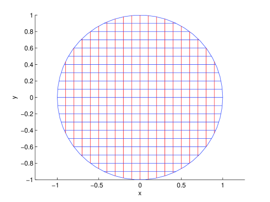
Figure 12: A grid on the unit disk

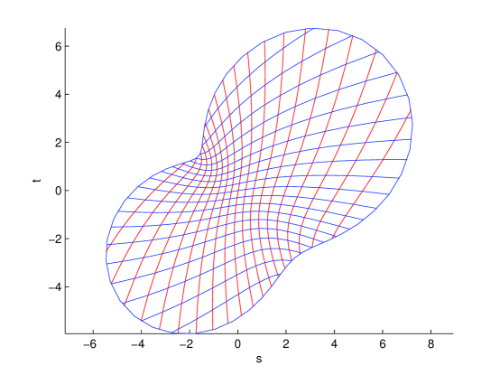
Figure 13: The image of the grid in Figure 12 under the mapping $\Phi_{3}^{(0)}$ for the domain given in (13).

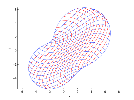
Figure 14: The image of the grid in Figure 12 under the final mapping $\Phi_{3}$.

5 Mapping in three dimensions

In this section we describe an algorithm to construct an extension $\Phi_{n}:B_{3}\mapsto\Omega$ for a given function $\varphi:S^{2}\mapsto\partial\Omega$. We assume that $\Omega$ is starlike with respect to the origin. The three dimensional case differs from the algorithm described in §4 in several ways. The dimension of $\Pi_{n}$ of the polynomials of maximal degree $n$ is given by $N_{n}={\binom{n}{3}}$, so any optimization algorithm has to deal with a larger number of degrees of freedom for a given $n$ when compared to the two dimensional case. Whereas in the two dimensional case a plot of $\boldsymbol{\Phi}_{n}(B_{2})$ reveals any problems of the constructed $\boldsymbol{\Phi}_{n}$ with respect to injectivity or $\boldsymbol{\Phi}_{n}(B_{2})\subset\Omega$ a similar plot of $\boldsymbol{\Phi}_{n}(B_{3})$ is not possible. For this reason, at the end of each optimization we calculate two measures which help us to decide if the constructed $\boldsymbol{\Phi}_{n}$ is injective and into.

On the other hand the principal approach to constructing $\boldsymbol{\Phi}_{n}$ is very similar to the algorithm described in §4. Again we are looking for a function $\boldsymbol{\Phi}_{n}$ given in the following form

$$\boldsymbol{\Phi}_{n}(x)=\sum_{j=1}^{N_{n}}\alpha_{n,j}\psi_{j}(x),\quad\quad x\in B_{3},$$

where $\{\psi_{1},\ldots,\psi_{N_{n}}\}$ is an orthonormal basis of $\Pi_{n}$ and the vectors $\alpha_{n,j}\in\mathbb{R}^{3}$, $j=1,\ldots,N_{n}$ are determined by an optimization algorithm.

For a given $n\in\mathbb{N}$ we use the extremal points of Womersley, see [9], on the sphere $S^{2}$. We will denote these points by $W_{n}=\{z_{1}^{(n)},\ldots,z_{(n+1)^{2}}^{(n)}\}$. These points guarantee that the smallest singular value of the interpolation matrix

$$A_{n}:=:\left[\begin{array}[c]{ccc}\psi_{1}(z_{1}^{(n)})&\ldots&\psi_{N_{n}}(z_{1}^{(n)})\\ \vdots&&\vdots\\ \psi_{1}(z_{(n+1)^{2}}^{(n)})&\ldots&\psi_{N_{n}}(z_{(n+1)^{2}}^{(n)})\end{array}\right]$$

stays above $1$ for all $n$ which we have used for our numerical examples. The number $(n+1)^{2}$ is also the largest possible number of interpolation points on the sphere which we can use, because $\dim(\Pi_{n}|_{S^{2}})=(n+1)^{2}$, see [3, Corollary 2.20 and formula (2.9)]. Again we enforce

$$\boldsymbol{\Phi}_{n}(z_{j}^{(n)})=\varphi(z_{j}^{(n)}),\quad\quad j=1,\ldots,(n+1)^{2},$$

for the mapping function $\boldsymbol{\Phi}_{n}$; see also (45). To define the initial function

$$\boldsymbol{\Phi}_{n}^{(0)}(x)=\sum_{j=1}^{N_{n}}\alpha_{n,j}^{(0)}\psi_{j}(x),\quad\quad x\in B_{3},$$ (49)

we choose

$$\alpha_{n,j}^{(0)}=(\widetilde{\Phi},\psi_{j})_{B_{3}},\quad\quad j=1\ldots,N_{n}.$$ (50)

$(\cdot,\cdot)_{B_{3}}$ is the usual $L_{2}$ inner product on $B_{3}$. The polynomial $\boldsymbol{\Phi}_{n}^{(0)}$ is the orthogonal projection of $\widetilde{\Phi}$ into $\Pi_{n}$. The function $\widetilde{\Phi}$ is some continuous extension of $\varphi$ to $B_{3}$, obtained by the generalization to three dimensions of one of the methods discussed in §§2,3. Having determined $\boldsymbol{\Phi}_{n}^{(0)}$, we convert the constrained optimization of the objective function $\Lambda(\cdot)$ into an unconstrained minimization, as discussed earlier in (45)-(47).

Once the Matlab program fminunc returns a local minimum for $\Lambda\left(\boldsymbol{\Phi}_{n}\right)$ and an associated minimizer $\boldsymbol{\Phi}_{n}$, we need to determine if $\boldsymbol{\Phi}_{n}$ satisfies

$$\boldsymbol{\Phi}_{n}(x) \neq\boldsymbol{\Phi}_{n}(y),\quad\quad x,y\in B_{3},\quad x\neq y,\quad\mbox{(injective)}$$ (51)

$$\boldsymbol{\Phi}_{n}(B_{3}) \subset\Omega,\quad\quad\mbox{(into)}$$ (52)

For this reason we calculate two measures of our mapping $\boldsymbol{\Phi}_{n}$.

Given $K\in\mathbb{N}$ we define a grid on the unit sphere,

$$\begin{array}[c]{r}S_{K}^{2}:=\left\{\left(\sin\left(\frac{1}{K}\pi j\right)\cos\left(\frac{1}{K}i\pi\right),\sin\left(\frac{1}{K}\pi j\right)\sin\left(\frac{1}{K}i\pi\right),\cos\left(\frac{1}{K}\pi j\right)\right)\,|\,\right.\vskip 3.0pt plus 1.0pt minus 1.0pt\\ \left.j=0,\ldots,K,\quad i=0,\ldots,2K-1^{\,{}^{\left.{}\right.}}\right\}.\end{array}$$

For $L\in\mathbb{N}$, we define a cubic grid in $B_{3},$

$$B_{3,L}:=\left(\frac{1}{L}\mathbb{Z}^{3}\right)\cap B_{3}$$

so every element in $B_{3,L}$ is given by

$$\begin{array}[c]{c}\frac{1}{L}(i,j,k),\quad\quad i,j,k\in\mathbb{Z},\vskip 3.0pt plus 1.0pt minus 1.0pt\\ i^{2}+j^{2}+k^{2}\leq L^{2}.\end{array}$$

To measure the minimum of the magnitude of the gradient of $\varphi$ over $S^{2}$, we define an approximation by

$$m_{K}(\varphi):=\displaystyle\min_{\begin{subarray}{c}x,y\in S_{K}^{2}\\ x\neq y\end{subarray}}\frac{\|\varphi(x)-\varphi(y)\|}{\|x-y\|}$$

This number is used to calculate

$$E_{1,K}(\boldsymbol{\Phi}_{n}):=\displaystyle\min_{\begin{subarray}{c}x,y\in B_{3,L},\\ x\neq y\end{subarray}}\frac{\|\boldsymbol{\Phi}_{n}(x)-\boldsymbol{\Phi}_{n}(y)\|}{\|x-y\|}\Big{/}m_{K}(\varphi)$$

Because of $\boldsymbol{\Phi}_{n}|_{S^{2}}\approx\varphi$ we expect $E_{1,K}\leq 1$. We use the occurrence of a very small value for $E_{1,K}(\boldsymbol{\Phi}_{n})$ to indicate that (51) may be violated. The result $E_{1,K}(\boldsymbol{\Phi}_{n})\approx 1$ is the best we can achieve, for example, with $\varphi$ and $\boldsymbol{\Phi}_{n}$ the identity mapping.

If (52) is violated there is a point $x\in B_{3}$ and a point $y\in S^{2}$ with $\boldsymbol{\Phi}_{n}(x)=\varphi(y)$. This shows that the following measure would be close to zero

$$E_{2,K,L}(\boldsymbol{\Phi}_{n}):=\displaystyle\min_{x\in B_{3,L},\,y\in S_{K}^{2}}\frac{\|\boldsymbol{\Phi}_{n}(x)-\varphi(y)\|}{\|x-y\|}\Big{/}m_{K}(\varphi)$$

Again we expect $E_{2,K,L}(\boldsymbol{\Phi}_{n})\leq 1$, and a very small value of $E_{2,K,L}(\boldsymbol{\Phi}_{n})$ indicates that (52) might be violated. For each $\boldsymbol{\Phi}_{n}$ which we calculate we will always report $E_{1,K}(\boldsymbol{\Phi}_{n})$ and $E_{2,K,L}(\boldsymbol{\Phi}_{n})$. For larger $K$ and $L$ we will get a more accurate test of the conditions (51) and (52), but the cost of calculation is rising, the complexity to calculate $E_{2,K,L}(\boldsymbol{\Phi}_{n})$ for example is $O(n^{3}K^{2}L^{3})$. For our numerical results we will use $K=40$ and $L=10$.

We consider only starlike examples for $\Omega$, with $\partial\Omega$ given as

$$\varphi\left(x\right) =\rho\left(x\right)x,\quad\quad x\in S^{2}$$

$$=\widehat{\rho}\left(\theta,\phi\right)\left(\sin\theta\cos\phi,\sin\theta\sin\phi,\cos\theta\right)$$ (53)

$$\widehat{\rho}\left(\theta,\phi\right)=\rho\left(\sin\theta\cos\phi,\sin\theta\sin\phi,\cos\theta\right)$$

To create an initial guess, we begin with the generalization of (6)-(7) to three dimensions, defined in the following way:

$$\widetilde{\Phi}\left(x\right) =r\widehat{\rho}\left(\theta,\phi\right)\left(\sin\theta\cos\phi,\sin\theta\sin\phi,\cos\theta\right)$$

$$=\widehat{\rho}\left(\theta,\phi\right)x$$

for $x=r\left(\sin\theta\cos\phi,\sin\theta\sin\phi,\cos\theta\right)$, $0\leq\theta\leq\pi,\ 0\leq\phi\leq 2\pi,\ 0\leq r\leq 1$. We assume $\rho:S^{2}\rightarrow\partial\Omega$ is a given smooth positive function. The initial guess $\boldsymbol{\Phi}_{n}^{\left(0\right)}$ is obtained using (49)-(50), the orthogonal projection of $\widetilde{\Phi}$ into $\Pi_{n}$. Even though $\widetilde{\Phi}$ is not continuously differentiable over $B_{3}$, its orthogonal projection $\boldsymbol{\Phi}_{n}^{\left(0\right)}$ is continuously differentiable, and it turns out to be a suitable initial guess with $\left.\boldsymbol{\Phi}_{n}^{\left(0\right)}\right|_{S^{2}}\approx\varphi$.

Example 17

In our first example we choose

$$\widehat{\rho}(\theta,\phi):=2+\left(\cos\theta\right)^{2}$$ (54)

Using $n=6$ yields the results given in Table 1 for the mapping $\Phi_{6}$ obtained using the optimization procedure described above.

Table 1: Measures of approximation stability for (54)

$\Lambda(\Phi_{6})$	$E_{1,40}(\Phi_{6})$	$E_{2,40,10}(\Phi_{6})$
$3.0575574308$	$0.7485506872$	$0.6626332145$

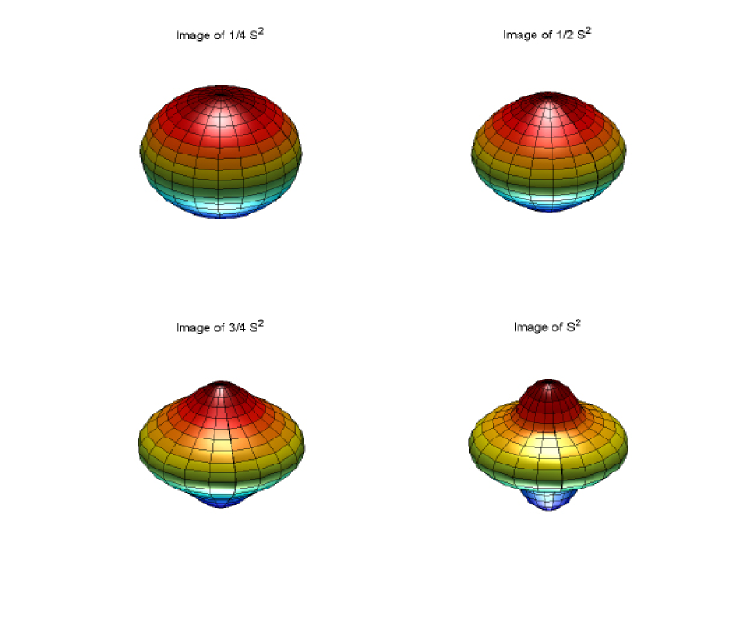
Figure 15: Images of $\frac{i}{4}S^{2}$, $i=1,2,3,4$

See Figure 15 for an illustration of the images of the various spheres $\frac{i}{4}S^{2}$.  In this example the initial mapping $\boldsymbol{\Phi}_{n}^{(0)}$ turned out to be a local optimum, so after the first iteration the optimization stopped. The measures $E_{1}$ and $E_{2}$ seem to indicate that the function $\boldsymbol{\Phi}_{n}^{(0)}$ is into $\Omega$ and injective. The error of $\Phi_{6}$ on the boundary is zero.

Example 18

Again the boundary $\partial\Omega$ is given by (53), but this time we choose

$$\widehat{\rho}(\theta,\phi):=2+\cos\theta+\frac{1}{2}\sin\theta\sin\phi$$ (55)

Using $n=6$ gives us the results shown in Table 2. We let $\Phi_{6}^{(0)}$ denote our initial guess for the iteration, derived as discussed earlier.

Table 2: Measures of approximation stability for (55)

Function	$\Lambda(\cdot)$	$E_{1,40}(\cdot)$	$E_{2,40,10}(\cdot)$
$\Phi_{6}^{(0)}$	$394.3717406299$	$0.2088413520$	$0.5926402745$
$\Phi_{6}$	$43.8782117161$	$0.2018029407$	$0.5175844592$

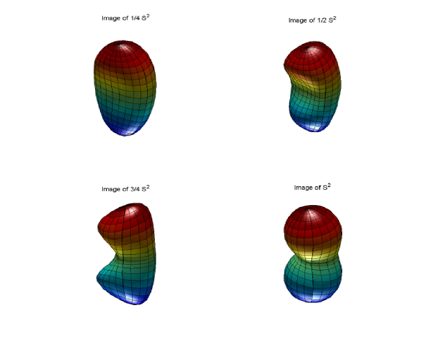
Figure 16: The images $\Phi^{\left(34\right)}\left(\frac{i}{4}S^{2}\right),$ $i=1,2,3,4$

See Figure 16 for an illustration of the images of the various spheres $\frac{i}{4}S^{2}$. In this example the $\Lambda(\cdot)$ value of the initial mapping $\Phi_{6}^{(0)}$ is significantly improved by the optimization. During the optimization the measures $E_{1}$ and $E_{2}$ do not approach zero, which indicates that $\Phi_{6}$ is a mapping from $B_{3}$ into $\Omega$ and is injective. The error of $\Phi_{6}^{(0)}$ and $\Phi_{6}$ on the boundary is zero.

References

- [1] K. Atkinson, D. Chien, and O. Hansen. A Spectral Method for Elliptic Equations: The Dirichlet Problem, Advances in Computational Mathematics, 33 (2010), pp. 169-189, DOI=10.1007/s10444-009-9125-8.
- [2] K. Atkinson and W. Han. On the numerical solution of some semilinear elliptic problems, Electronic Transactions on Numerical Analysis 17 (2004), pp. 206-217.
- [3] K. Atkinson and W. Han. Approximation on the Unit Sphere, to be published.
- [4] K. Atkinson and O. Hansen. A Spectral Method for the Eigenvalue Problem for Elliptic Equations, Electronic Transactions on Numerical Analysis 37 (2010), pp. 386-412.
- [5] K. Atkinson,O. Hansen, and D. Chien. A Spectral Method for Elliptic Equations: The Neumann Problem, Advances in Computational Mathematics, 34 (2011), pp. 295-317, DOI=10.1007/s10444-010-9154-3.
- [6] B. Logan and L. Shepp. Optimal reconstruction of a function from its projections, Duke Math. J. 42, (1975), 645–659.
- [7] J. Nocedal and S.J. Wright Numerical Optimization, Springer–Verlag New York, Inc., 1999.
- [8] A. Stroud. Approximate Calculation of Multiple Integrals, Prentice-Hall, Inc., Englewood Cliffs, N.J., 1971.
- [9] R. Womersley. Extremal (Maximum Determinant) points on the sphere , http://web.maths.unsw.edu.au/rsw/Sphere/Extremal/New/extremal1.html
- [10] E. Zeidler. Nonlinear Functional Analysis and its Applications I, Springer–Verlag, New York Inc, 1986.