A polyhedral approach for the Equitable Coloring Problem

Abstract

In this work we study the polytope associated with a 0,1-integer programming formulation for the Equitable Coloring Problem. We find several families of valid inequalities and derive sufficient conditions in order to be facet-defining inequalities. We also present computational evidence that shows the efficacy of these inequalities used in a cutting-plane algorithm.

1 Introduction

In graph theory, there is a large family of optimization problems having relevant practical importance, besides its theoretical interest. One of the most representative problem of this family is the Graph Coloring Problem (GCP), which arises in many applications such as scheduling, timetabling, electronic bandwidth allocation and sequencing problems.

Given a simple graph $G=(V,E)$, where $V$ is the set of vertices and $E$ is the set of edges, a coloring of $G$ is an assignment of colors to each vertex such that the endpoints of any edge have different colors. A $k$-coloring is a coloring that uses $k$ colors. Equivalently, a $k$-coloring can be defined as a partition of $V$ into $k$ subsets, called color classes, such that adjacent vertices belong to different classes. Given a $k$-coloring, color classes are denoted by $C_{1},\ldots,C_{k}$ assuming that, for each $i\in\{1,\ldots,k\}$, vertices in $C_{i}$ are colored with color $i$. We can also define a $k$-coloring of $G$ as a mapping $c:V\rightarrow\{1,\ldots,k\}$ such that $c(u)\neq c(v)$ for all $(u,v)\in E$. The GCP consists of finding the minimum number of colors such that a coloring exists. This minimum number of colors is called the chromatic number of the graph $G$ and is denoted by $\chi(G)$.

Some applications impose additional restrictions arising variations of GCP. For instance, in scheduling problems, it may be required to ensure the uniformity of the distribution of workload employees. The addition of these extra equity constraints gives rise to the Equitable Coloring Problem (ECP). An equitable $k$-coloring (or just $k$-eqcol) of $G$ is a $k$-coloring satisfying the equity constraints, i.e. $\left||C_{i}|-|C_{j}|\right|\leq 1$, for $i,j\in\{1,\ldots,k\}$ or, equivalently, $\lfloor n/k\rfloor\leq|C_{j}|\leq\lceil n/k\rceil$ for each $j\in\{1,\ldots,k\}$. The equitable chromatic number of $G$, $\chi_{eq}(G)$, is the minimum $k$ for which $G$ admits a $k$-eqcol. The ECP consists of finding $\chi_{eq}(G)$.

The ECP was introduced in [12], motivated by an application concerning garbage collection [14]. Other applications of the ECP concern load balancing problems in multiprocessor machines [4] and results in probability theory [13]. An introduction to ECP and some basics results are provided in [6].

Computing $\chi_{eq}(G)$ for arbitrary graphs is proved to be $NP$-hard and just a few families of graphs are known to be easy such as complete $n$-partite, complete split, wheel and tree graphs [6]. In particular, if $G$ has a universal vertex $u$, the cardinality of the color classes of any equitable coloring in $G$ is at most two and the color classes of exactly two vertices correspond to a matching in the complement of $G$. In other words, the ECP is polynomial when $G$ has at least one universal vertex.

There exist some remarkable differences between GCP and ECP. Unlike GCP, a graph admiting a $k$-eqcol may not admit a $(k+1)$-eqcol. This leads us to define the skip set of $G$, $\mathscr{S}(G)$, as the set of $k\in\{\chi_{eq}(G),\ldots,n\}$ such that $G$ does not admit any $k$-eqcol. For instance, if $G=K_{3,3}$, i.e. the complete bipartite graph with partitions of size 3, then $G$ admits a 2-eqcol but does not admit a 3-eqcol. Here, $\mathscr{S}(K_{3,3})=\{3\}$. Computing the skip set of a graph is as hard as computing the equitable chromatic number. If $\mathscr{S}(G)=\varnothing$, we say that $G$ is monotone. For instance, trees are monotone graphs [7].

Another drawback emerging from ECP is that the equitable chromatic number of a graph can be smaller than the equitable chromatic number of one of its induced subgraphs. In particular, in an unconnected graph, equitable chromatic numbers of each connected component are uncorrelated with the chromatic number of the whole graph.

On the other hand, some useful properties of GCP also hold for ECP. For example, it is known that $G$ admits $k$-eqcols for $k\geq\Delta(G)+1$, where $\Delta(G)$ is the maximum degree of vertices in $G$. In [5] a polynomial time algorithm which produces a $(\Delta(G)+1)$-eqcol is presented.

Integer linear programming (ILP) approach together with algorithms which exploit the polyhedral structure proved to be the best tool for dealing with coloring problems. Although many ILP formulations are known for GCP, as far as we know, just two of these models were adapted for ECP. One of them, given in [2], is based on the asymmetric representatives model for the GCP [3]. The other one, proposed by us in [9], is based on the classic color assignments to vertices model [1] with further improvements stated in [11].

The goal of this paper is to study the last model from a polyhedral point of view and determine families of valid inequalities which can be useful in the context of an efficient cutting-plane algorithm.

The remainder of the paper is organized as follows.

In sections 2-3, we study the facial structure of the polytope associated with the formulation given in [9]. We introduce several families of valid inequalities which always define high dimensional faces. Section 4 is devoted to describe a cutting-plane algorithm for solving ECP. We expose computational evidence for reflecting the improvement in the performance when the cutting-plane algorithm uses the new inequalities as cuts. That algorithm is then used to reinforce bounds on a Branch and Bound enumeration tree. At the end, a conclusion is presented.

Some definitions and notations will be useful in the following.

Given a graph $G=(V,E)$ we consider $V=\{1,\ldots,n\}$. The complement of $G$ is denoted by $\overline{G}$. We also denote by $K_{n}$ the complete graph of $n$ vertices. The percentage of density of $G$ is $\dfrac{100|E|}{|V|(|V|-1)/2}$. For instance, the percentage of density of any complete graph is 100. Given $u\in V$, the degree of $u$ is the number of vertices adjacent to $u$ and is denoted by $\delta(u)$. For any $S\subset V$, $G[S]$ is the graph induced by $S$ and $G-S$ is the graph obtained by the deletion of vertices in $S$, i.e. $G-S=G[V\backslash S]$. In particular, if $S=\{u\}$ we just write $G-u$ instead of $G-\{u\}$. A stable set is a set of vertices in $G$, no two of which are adjacent. We denote by $\alpha(G)$ the stability number of $G$, i.e. the maximum cardinality of a stable set of $G$. Given $S\subset V$, we also denote by $\alpha(S)$ the stability number of $G[S]$. We say that $S$ is $k$-maximal if $\alpha(S)=k$ and for all $v\in V\backslash S$, $\alpha(S\cup\{v\})=k+1$. In particular, if $S$ is 1-maximal, we say that $S$ is a maximal clique. Given $u\in V$, the neighborhood of $u$, $N(u)$, is the set of vertices adjacent to $u$, and the closed neighborhood of $u$, $N[u]$, is the set $N(u)\cup\{u\}$. A vertex $u\in V$ is a universal vertex if $N[u]=V$. A matching of $G$ is a subset of edges such that no pair of them has a common extreme point. Whenever it is clear from the context, we will write $\chi_{eq}$ rather than $\chi_{eq}(G)$. The same convention also applies for other operators that depend on $G$ such as $\mathscr{S}$ and $\Delta$.

Throughout the paper, we consider graphs with at least five vertices and one edge, and not containing universal vertices nor $K_{n-1}$ as an induced subgraph. Thus, for a given graph $G$ we assume that $2\leq\chi_{eq}(G)\leq n-2$. The remaining cases can be solved in polynomial time.

2 The polytope $\mathcal{ECP}$

A straightforward ILP model for GCP can be obtained by modeling colorings with two sets of binary variables: variables $x_{vj}$ for $v\in V$ and $j\in\{1,\ldots,n\}$ where $x_{vj}=1$ if and only if the coloring assigns color $j$ to vertex $v$, and variables $w_{j}$ for $j\in\{1,\ldots,n\}$ where $w_{j}=1$ if and only if color $j$ is used in the coloring. The formulation is shown below:

$$\sum_{j=1}^{n}x_{vj}=1, \forall~{}v\in V$$ (1)

$$x_{uj}+x_{vj}\leq w_{j}, \forall~{}(u,v)\in E,~{}1\leq j\leq n$$ (2)

Constraints (1) assert that each vertex has to be colored by a unique color and constraints (2) ensure that two adjacent vertices can not share the same color. Hence, the chromatic number can be computed by minimizing $\sum_{j=1}^{n}w_{j}$.

This formulation presents a disadvantage: the number of integer solutions $(x,w)$ with the same value $\sum_{j=1}^{n}w_{j}$ is very large. A technique widely used in combinatorial optimization to deal with this kind of problem is the concept of symmetry breaking [8]. This technique is applied in [11], where the following constraints are added to the previous formulation in order to remove (partially) symmetric solutions:

$$w_{j+1}\leq w_{j}, \forall~{}1\leq j\leq n-1$$ (3)

which means that color $j+1$ may be used only if color $j$ is also used.

Given a partition of $V$ into color classes, let us observe that permutations of colors between those sets yield symmetric colorings. In [11], additional constraints are proposed in order to drop most of these colorings by sorting the color classes by the minimum label of the vertices belonging to each set and only considering the coloring that assigns color $j$ to the $j$th color class. These constraints are:

$$x_{vj}=0, \forall~{}1\leq v<j\leq n$$ (4)

$$x_{vj}\leq\sum_{u=j-1}^{v-1}x_{uj-1}, \forall~{}2\leq j\leq v\leq n$$ (5)

Even though the formulation consisting of constraints (1)-(5) eliminates a greater amount of symmetrical solutions, it is difficult to characterize the integer polyhedron associated to that formulation since it depends on the labeling of vertices [11].

From now on, we represent colorings of $G$ as binary vectors $(x,w)$ satisfying constraints (1)-(3) and we call Coloring Polytope, $\mathcal{CP}(G)$, to the convex hull of binary vectors $(x,w)$ that represent colorings of $G$.

In order to characterize equitable colorings, we add the following constraints to the model:

$$x_{vj}\leq w_{j}, \forall~{}v~{}\textrm{isolated},~{}1\leq j\leq n$$ (6)

$$\sum_{v\in V}x_{vj}\geq\sum_{k=j}^{n}\biggl{\lfloor}\dfrac{n}{k}\biggr{\rfloor}\bigl{(}w_{k}-w_{k+1}\bigr{)}, \forall~{}1\leq j\leq n-1$$ (7)

$$\sum_{v\in V}x_{vj}\leq\sum_{k=j}^{n}\biggl{\lceil}\dfrac{n}{k}\biggr{\rceil}\bigl{(}w_{k}-w_{k+1}\bigr{)}, \forall~{}1\leq j\leq n-1$$ (8)

where $w_{n+1}$ is a dummy variable set to 0. Constraints (6) ensure that isolated vertices use enabled colors and (7)-(8) are precisely the equity constraints. The Equitable Coloring Polytope $\mathcal{ECP}(G)$ is defined as the convex hull of binary vectors $(x,w)$ that represent equitable colorings of $G$, i.e. they satisfy constraints (1)-(3) and (6)-(8).

From now on, we present equitable colorings by using mappings, color classes or binary vectors, according to our convenience.

We also work with two useful operators over colorings. The first one is based on the fact that swapping colors in a $k$-eqcol produces a $k$-eqcol indeed.

Definition 1.

Let $c$ be a $k$-eqcol of $G$ with color classes $C_{1}$, $\ldots$, $C_{k}$ and $L=(j_{1},j_{2},\ldots,j_{r})$ be an ordered list of different colors in $\{1,\ldots,k\}$. We define $swap_{L}(c)$ as the $k$-eqcol with color classes $C^{\prime}_{1}$, $\ldots$, $C^{\prime}_{k}$ which satisfies $C^{\prime}_{j_{t}}=C_{j_{t+1}}~{}~{}\forall~{}1\leq t\leq r-1$, $C^{\prime}_{j_{r}}=C_{j_{1}}$ and $C^{\prime}_{i}=C_{i}~{}~{}\forall~{}i\in\{1,2,\ldots,k\}\backslash\{j_{1},j_{2},\ldots,j_{r}\}$.

The other operator takes a $k$-eqcol whose color classes have at most 2 vertices and returns a $(k+1)$-eqcol.

Definition 2.

Let $c$ be a $k$-eqcol of $G$ with $\lceil n/2\rceil\leq k\leq n-1$ and $v\neq v^{\prime}$ such that $c(v)=c(v^{\prime})$. We define $intro(c,v)$ as a $(k+1)$-eqcol $c^{\prime}$ which satisfies $c^{\prime}(v)=k+1$ and $c^{\prime}(i)=c(i)~{}~{}\forall~{}i\in V\backslash\{v\}$.

Remark 3.

Let us observe that colorings with $n-1$ and $n$ colors are always equitable. Then, we can use Proposition 1 of [11] to prove that the following $n^{2}-\chi_{eq}-|\mathscr{S}|$ equitable colorings are affinely independent:

1. A $(n-1)$-eqcol $c$ such that $C_{n-1}$ has two vertices, namely $u_{1}$ and $u_{2}$.

2. $swap_{n-1,j}(c)$ for each $j\in\{1,\ldots,n-2\}$.

3. The $n$-eqcol $c^{\prime}=intro(c,u_{1})$.

4. $swap_{n,j,j^{\prime}}(c^{\prime})$ for each $j,j^{\prime}\in\{1,\ldots,n-1\}$ such that $j^{\prime}\neq j$.

5. $swap_{n,j}(c^{\prime})$ for each $j\in\{1,\ldots,n-1\}$.

6. An arbitrary $k$-eqcol of $G$ for each $k\in\{\chi_{eq},\ldots,n-2\}\backslash\mathscr{S}$.

Theorem 4.

The dimension of $\mathcal{ECP}$ is $n^{2}-(\chi_{eq}+|\mathscr{S}|+1)$ and a minimal equation system is defined by:

$$\sum_{j=1}^{n}x_{vj}=1, \forall~{}v\in V,$$ (9)

$$w_{j}=1, \forall~{}1\leq j\leq\chi_{eq},$$ (10)

$$w_{j}=w_{j+1}, \forall~{}j\in\mathscr{S},$$ (11)

$$\sum_{v\in V}x_{vn}=w_{n}.$$ (12)

Proof.

From Remark 3, $dim(\mathcal{ECP})\geq n^{2}-(\chi_{eq}+|\mathscr{S}|+1)$. We only need to note that $\mathcal{ECP}\subset\mathbb{R}^{n^{2}+n}$ and that every equitable coloring satisfies $n+\chi_{eq}+\mathscr{S}+1$ mutually independent equalities given in (9)-(12). ∎

Let us analyze the faces of $\mathcal{ECP}$ defined by restrictions of the formulation. For non-negativity constraints and inequalities (3) we adapt the proofs given in [11] for $\mathcal{CP}$.

Theorem 5.

Let $v\in V$ and $1\leq j\leq n$. Constraint $x_{vj}\geq 0$ defines a facet of $\mathcal{ECP}$.

Proof.

We exhibit $n^{2}-\chi_{eq}-|\mathscr{S}|-1$ affinely independent colorings that lie on the face of $\mathcal{ECP}$ defined by inequality $x_{vj}\geq 0$. Let us consider the following cases:
Case $j\leq n-2$. Let $u_{1},u_{2}\in V\backslash\{v\}$ be non adjacent vertices and let $c$ be a $(n-1)$-eqcol such that $c(v)\neq j$ and $C_{n-1}=\{u_{1},u_{2}\}$. We consider the set of colorings given by Remark 3 starting with $c$ and choosing the arbitrary $k$-eqcols in item 6 satisfying that vertex $v$ is not painted with color $j$. It is clear that all these colorings, except $swap_{n,j,c(v)}(c^{\prime})$ where $c^{\prime}=intro(c,u_{1})$, lie in the face defined by the inequality.
Case $j=n-1$. Let $S$ be the set of $n$-eqcols and $(n-1)$-eqcols presented in the previous case for $j=n-2$. We consider the colorings $swap_{n-1,n-2}(\tilde{c})$ for each $\tilde{c}\in S$ and an arbitrary $k$-eqcol of $G$ for each $k\in\{\chi_{eq},\ldots,n-2\}\backslash\mathscr{S}$.
Case $j=n$. Let $u_{2}$ be a vertex not adjacent to $v$. We consider the set of colorings given by Remark 3 starting with a $(n-1)$-eqcol $c$ such that $C_{n-1}=\{v,u_{2}\}$. It is clear that all these colorings, except $intro(c,v)$, lie in the face defined by the inequality. ∎

Let $1\leq j\leq n-1$ and $\mathcal{F}$ be the face of $\mathcal{ECP}$ defined by constraint (3), i.e. $w_{j+1}\leq w_{j}$. Let us notice that, if $G$ does not admit a $j$-eqcol, i.e. $j\in\{1,\ldots,\chi_{eq}-1\}\cup\mathscr{S}$, then (3) is a linear combination of equations of the minimal system and, therefore, $\mathcal{F}=\mathcal{ECP}$. In addition, if $j=n-1$, the class of color $n-1$ of every coloring $(x,w)$ satisfying $w_{n}=w_{n-1}$ have at most one vertex and, therefore, $(x,w)$ verifies $\sum_{v\in V}x_{vn-1}=w_{n-1}$. Then, $\mathcal{F}$ is not a facet of $\mathcal{ECP}$. For the remaining cases, we have the following result.

Theorem 6.

If $G$ admits a $j$-eqcol and $j\leq n-2$, constraint $w_{j+1}\leq w_{j}$ defines a facet of $\mathcal{ECP}$.

Proof.

Let us consider the set of colorings from Remark 3 but excluding the $j$-eqcol from item 6. Clearly, the remaining colorings lie on the face and (3) defines a facet of $\mathcal{ECP}$. ∎

The following theorems are related to the faces of $\mathcal{ECP}$ defined by the equity constraints.

Theorem 7.

Let $1\leq j\leq n-1$. Constraint

$$\sum_{v\in V}x_{vj}\geq\sum_{k=j}^{n}\biggl{\lfloor}\frac{n}{k}\biggr{\rfloor}(w_{k}-w_{k+1})$$

defines a facet of $\mathcal{ECP}$.

Proof.

Let $u_{1},u_{2}$ be non adjacent vertices and let $c$ be a $(n-1)$-eqcol $c$ such that $C_{n-1}=\{u_{1},u_{2}\}$. We consider the set of colorings given by Remark 3 starting with $c$ and choosing $k$-eqcols in item 6 satisfying $|C_{j}|=\lfloor n/k\rfloor$ when $k\geq j$. The proposed colorings, except the $(n-1)$-eqcol that satisfies $C_{j}=\{u_{1},u_{2}\}$, lie on the face and therefore (7) defines a facet of $\mathcal{ECP}$. ∎

Let us observe that if $1\leq j\leq n-2$, the face of $\mathcal{ECP}$ defined by (8) is not a facet. Indeed, every coloring $(x,w)$ lying on the face satisfies $\sum_{v\in V}x_{vn-1}=w_{n-1}$. For the case $j=n-1$, the constraint (8) is $\sum_{v\in V}x_{vn-1}\leq 2w_{n-1}-w_{n}$ and we have:

Theorem 8.

The inequality $\sum_{v\in V}x_{vn-1}\leq 2w_{n-1}-w_{n}$ defines a facet of $\mathcal{ECP}$.

Proof.

Since $n\geq 5$ and $\chi_{eq}(G)\leq n-2$ there exist $u_{1},u_{2},u_{3},u_{4},u_{5}\in V$ such that $u_{1}$ is not adjacent to $u_{2}$ and $u_{3}$ is not adjacent to $u_{4}$. Let $c$ be a $(n-1)$-eqcol $c$ such that $c(u_{1})=c(u_{2})=n-1$. We consider the colorings from items 1,3,4,5 in Remark 3 together with the following ones:

• The $(n-2)$-eqcol $\hat{c}$ such that $\hat{c}(u_{1})=\hat{c}(u_{2})=c(u_{3})$, $\hat{c}(u_{3})=c(u_{4})$ and $\hat{c}(i)=c(i)~{}~{}\forall~{}i\in V\backslash\{u_{1},u_{2},u_{3}\}$.

• $swap_{j,c(u_{3})}(\hat{c})$ for each $j\in\{1,\ldots,n-2\}\backslash\{c(u_{3}),c(u_{4})\}$.

• $swap_{\hat{c}(u_{5}),c(u_{4})}(\hat{c})$.

• An arbitrary $k$-eqcol of $G$ for each $k\in\{\chi_{eq},\ldots,n-3\}\backslash\mathscr{S}$.

The proof for the affine independence of the previous $n^{2}-\chi_{eq}-|\mathscr{S}|-1$ colorings is similar to the one for the colorings generated in Remark 3. ∎

2.1 Valid inequalities from $\mathcal{CP}$

Taking into account that valid inequalities for $\mathcal{CP}$ are also valid for $\mathcal{ECP}$, in this section we analyze the faces of $\mathcal{ECP}$ defined by facet-defining inequalities of $\mathcal{CP}$.

One of the families of valid inequalities presented in [11] is the following. Given a vertex $v$ and a color $j$, the $(v,j)$-block inequality is $\sum_{k=j}^{n}x_{vk}\leq w_{j}$.

Let us observe that the $(v,1)$-block inequality is always satisfied by equality since every coloring $(x,w)$ verifies constraints (1) and $w_{1}=1$. Moreover, the $(v,2)$-block inequality defines the same facet as inequality $x_{v1}\geq 0$. For the remaining cases we have:

Theorem 9.

Let $v\in V$ and $3\leq j\leq n-2$. The $(v,j)$-block inequality defines a facet of $\mathcal{ECP}$ if and only if $G$ admits a $(j-1)$-eqcol.

Proof.

Let $\mathcal{F}$ be the face of $\mathcal{ECP}$ defined by the $(v,j)$-block inequality. To prove that $\mathcal{F}$ is a facet of $\mathcal{ECP}$ when $G$ admits a $(j-1)$-eqcol, we can use the same affinely independent colorings proposed in the proof of Proposition 10 of [11], by imposing them to be equitable colorings.
Now, let us suppose that $G$ does not admit a $(j-1)$-eqcol. We will prove that every equitable coloring lying on the face satisfies $x_{vj-1}=0$. Let $(x,w)$ be a $k$-eqcol lying on $\mathcal{F}$. If $k\leq j-2$, clearly $x_{vj-1}=0$. Otherwise, $\sum_{k=j}^{n}x_{vk}=1$ since $k\neq j-1$, and then $x_{vj-1}=0$. ∎

Let us consider other family of inequalities studied in [11]. Given $S\subset V$ and a color $j$, $\sum_{v\in S}x_{vj}\leq\alpha(S)w_{j}$ is valid for $\mathcal{CP}$. The authors of [11] proved that, by applying a lifting procedure on this inequality for $j\leq n-\alpha(S)$, we can get

$$\sum_{v\in S}x_{vj}+\sum_{v\in V}\sum_{k=n-\alpha(S)+1}^{n-1}x_{vk}\leq\alpha(S)w_{j}+w_{n-\alpha(S)+1}-w_{n}.$$

We will refer to it as the $(S,j)$-rank inequality.

Let us remark that, if $S$ is not $\alpha(S)$-maximal, i.e. if there exists $v\in V\backslash S$ such that $\alpha(S\cup\{v\})=\alpha(S)$, the $(S,j)$-rank inequality is dominated by the $(S\cup\{v\})$-rank inequality. Then, from now on, we only consider $(S,j)$-rank inequalities where $S$ is $\alpha(S)$-maximal.

When $\alpha(S)=1$, the $(S,j)$-rank inequality takes the form $\sum_{v\in S}x_{vj}\leq w_{j}$ and is called $(S,j)$-clique inequality. If $|S|=1$, i.e. $S=\{v\}$ for some $v$, the $(S,j)$-clique inequality is dominated by the $(v,j)$-block inequality. If $|S|\geq 2$, Propositions 5 and 6 of [11] state that the $(S,j)$-clique inequality defines a facet of $\mathcal{CP}$. The proof of these propositions can be easily adapted to the equitable case allowing us to prove the following result.

Theorem 10.

Let $Q$ be a maximal clique of $G$ with $|Q|\geq 2$ and $j\leq n-1$. The $(Q,j)$-clique inequality defines a facet of $\mathcal{ECP}$.

In Theorem 33 of [10] we give sufficient conditions for the $(S,j)$-rank inequalities to define facets of $\mathcal{ECP}$ when $\alpha(S)=2$.

Other valid inequalities can arise when $\alpha(S)=2$. Let $Q$ be the set of vertices of $S$ that are universal in $G[S]$, i.e. $Q=\{q\in S~{}:~{}S\subset N[q]\}$. If $Q$ is not empty, we may apply a different lifting procedure that one used in [11], obtaining new valid inequalities for $\mathcal{CP}$ and $\mathcal{ECP}$:

Definition 11.

The $(S,Q,j)$-2-rank inequality is defined for a given $S\subset V$ such that $S$ is 2-maximal, $Q=\{q\in S~{}:~{}S\subset N[q]\}\neq\varnothing$ and $j\leq n-1$, as

$$\sum_{v\in S\backslash Q}x_{vj}+2\sum_{v\in Q}x_{vj}\leq 2w_{j}.$$ (13)

Lemma 12.

The $(S,Q,j)$-2-rank inequality is valid for $\mathcal{ECP}$.

Proof.

If some vertex of $Q$ uses color $j$, no one else in $S$ can be painted with $j$. Therefore, the value of the l.h.s. in (13) is at most 2 when color $j$ is used. ∎

If $|Q|=1$, the $(S,Q,j)$-2-rank inequality is dominated by another valid inequality presented in the next section (see Remark 17).

In Theorem 34 and Corollary 35 of [10], we give sufficient conditions for the $(S,Q,j)$-2-rank inequalities to define facets of $\mathcal{ECP}$ when $|Q|\geq 2$.

3 New valid inequalities for $\mathcal{ECP}$

In this section, we present new families of valid inequalities for $\mathcal{ECP}$ which are not valid for $\mathcal{CP}$.

3.1 Subneighborhood inequalities

The neighborhood inequalities defined in [11] for each $u\in V$, i.e. $\alpha(N(u))x_{uj}$ $+\sum_{v\in N(u)}x_{vj}\leq\alpha(N(u))w_{j}$, are valid inequalities for $\mathcal{CP}$. Indeed, if $S\subset N(u)$, $\alpha(S)x_{uj}+\sum_{v\in S}x_{vj}\leq\alpha(S)w_{j}$ is valid for $\mathcal{CP}$. We can reinforce the latter inequality in the context of $\mathcal{ECP}$ to obtain:

Definition 13.

The $(u,j,S)$-subneighborhood inequality is defined for a given $u\in V$, $S\subset N(u)$ such that $S$ is not a clique and $j\leq n-1$, as

$$\gamma_{jS}x_{uj}+\sum_{v\in S}x_{vj}+\sum_{k=j+1}^{n}(\gamma_{jS}-\gamma_{kS})x_{uk}\leq\gamma_{jS}w_{j},$$ (14)

where $\gamma_{kS}=\min\{\lceil n/\chi_{eq}\rceil,\lceil n/k\rceil,\alpha(S)\}$.

Lemma 14.

The $(u,j,S)$-subneighborhood inequality is valid for $\mathcal{ECP}$.

Proof.

Let $(x,w)$ be an $r$-eqcol of $G$. If $r<j$, both sides of (14) are equal to zero. If $r\geq j$ and $x_{uj}=1$, the value of the l.h.s. of (14) is exactly $\gamma_{jS}$. On the other hand, if $x_{uj}=0$, the term $\sum_{v\in S}x_{vj}$ contributes up to $\gamma_{rS}$ and the term $\sum_{k=j+1}^{n}(\gamma_{jS}-\gamma_{kS})x_{uk}$ contributes up to $\gamma_{jS}-\gamma_{rS}$ regardless the color assigned to $u$. Hence, the l.h.s. does not exceed $\gamma_{jS}$ and (14) is valid. ∎

Subneighborhood inequalities always define faces of high dimension:

Theorem 15.

Let $\mathcal{F}$ be the face defined by the $(u,j,S)$-subneighborhood inequality. Then,

$$dim(\mathcal{F})\geq dim(\mathcal{ECP})-\bigl{(}\lceil n/2\rceil-1-|S|+\delta(u)\bigr{)}=o(dim(\mathcal{ECP})).$$

Proof.

Let $s_{1},s_{2}\in S$ be non adjacent vertices and let $1\leq r\leq\lceil n/2\rceil-1$ such that $r\neq j$. We propose at least $n^{2}-\lceil n/2\rceil-\chi_{eq}-|\mathscr{S}|+|S|-\delta(u)+1$ affinely independent colorings lying on $\mathcal{F}$.

• A $n$-eqcol $c$ such that $c(u)=j$, $c(s_{1})=n$ and $c(s_{2})=r$.

• $swap_{n,j_{1},j_{2}}(c)$ for each $j_{1},j_{2}\in\{1,\ldots,n-1\}\backslash\{j\}$ such that $j_{1}\neq j_{2}$.

• $swap_{c(s),n,j}(c)$ for each $s\in S\backslash\{s_{1}\}$.

• $swap_{n,j^{\prime}}(c)$ for each $j^{\prime}\in\{1,\ldots,n-1\}$.

• The $(n-1)$-eqcol $c^{\prime}$ such that $c^{\prime}(s_{1})=r$ and $c^{\prime}(i)=c(i)~{}~{}\forall~{}i\in V\backslash\{s_{1}\}$.

• $swap_{j^{\prime},r}(c^{\prime})$ for each $j^{\prime}\in\{1,\ldots,n-1\}\backslash\{j,r\}$.

• $swap_{j,r,j^{\prime}}(c^{\prime})$ for each $j^{\prime}\in\{1,\ldots,n-1\}\backslash\{j,r\}$ and, if $j\leq\lceil n/2\rceil-1$ then $j^{\prime}\geq\lceil n/2\rceil$.

• The $(n-1)$-eqcol $c^{\prime\prime}$ such that $c^{\prime\prime}(s_{1})=c(v)$, $c^{\prime\prime}(v)=j$ and $c^{\prime\prime}(i)=c(i)~{}~{}\forall~{}i\in V\backslash\{s_{1},v\}$, for each $v\in V\backslash N[u]$.

• If $j\geq\chi_{eq}+1$, an arbitrary $k$-eqcol of $G$ for each $k\in\{\chi_{eq},\ldots,j-1\}\backslash\mathscr{S}$.

• $swap_{j,\hat{c}(u)}(\hat{c})$ where $\hat{c}$ is a $k$-eqcol of $G$, for each $k\in\bigl{\{}\max\{j,\chi_{eq}\},\ldots,n-2\bigr{\}}\backslash\mathscr{S}$.

The proof for the affine independence of the previous colorings is similar to the one for the colorings generated in Remark 3. ∎

Sufficient conditions for a $(u,j,S)$-subneighborhood inequality to be a facet-defining inequality of $\mathcal{ECP}$ are presented in Theorem 36 of [10] for the case $\lceil n/j\rceil\leq\lceil n/\chi_{eq}\rceil$ whereas the following result allows us to study the inequality for the case $\lceil n/j\rceil>\lceil n/\chi_{eq}\rceil$.

Theorem 16.

Let $j$ such that $\lceil n/j\rceil>\lceil n/\chi_{eq}\rceil$, $\mathcal{F}_{j}$ be the face defined by the $(u,j,S)$-subneighborhood inequality and $\mathcal{F}_{\chi_{eq}}$ be the face defined by the $(u,\chi_{eq},S)$-subneighborhood inequality. Then, $dim(\mathcal{F}_{j})=dim(\mathcal{F}_{\chi_{eq}})$.

Proof.

Clearly, if $\alpha(S)<\lceil n/\chi_{eq}\rceil$, both inequalities coincide. So, let us assume that $\alpha(S)\geq\lceil n/\chi_{eq}\rceil$. Since $\lceil n/j\rceil>\lceil n/\chi_{eq}\rceil$, $j<\chi_{eq}$ and $w_{j}=w_{\chi_{eq}}=1$. Then, both inequalities only differ in the coefficients of $x_{vj}$ and $x_{v\chi_{eq}}$ for all $v\in V$. Moreover, the coefficient of $x_{vj}$ in the $(u,j,S)$-subneighborhood is the same as the one of $x_{v\chi_{eq}}$ in the $(u,\chi_{eq},S)$-subneighborhood, and conversely.
Let $d=dim(\mathcal{F}_{\chi_{eq}})$ and $d^{\prime}=dim(\mathcal{F}_{j})$. If $c^{1},c^{2},\ldots,c^{d+1}$ are affinely independent equitable colorings in $\mathcal{F}_{\chi_{eq}}$, colorings $swap_{j,\chi_{eq}}(c^{i})$ for $1\leq i\leq d+1$ are well defined and they are affinely independent too. Moreover, they lie on $\mathcal{F}_{j}$. Therefore, $d\leq d^{\prime}$.
To prove that $d^{\prime}\leq d$, we follow the same reasoning. ∎

Remark 17.

Let $j\leq n-1$, $S\subset V$ such that $\alpha(S)=2$ and $Q=\{v\in S~{}:~{}S\subset N[v]\}=\{q\}$. The $(q,j,S\backslash\{q\})$-subneighborhood inequality is

$$\sum_{v\in S\backslash\{q\}}x_{vj}+2x_{qj}+x_{qn}\leq 2w_{j},$$

and dominates the $(S,Q,j)$-2-rank inequality. In Corollary 37 of [10] we give sufficient conditions for it to be a facet-defining inequality of $\mathcal{ECP}$.

3.2 Outside-neighborhood inequalities

Definition 18.

The $(u,j)$-outside-neighborhood inequality is defined for a given $u\in V$ such that $N(u)$ is not a clique and $j\leq\lfloor n/2\rfloor$, as

$$\biggl{(}\biggl{\lfloor}\dfrac{n}{t_{j}}\biggr{\rfloor}-1\biggr{)}x_{uj}-\sum_{v\in V\backslash N[u]}x_{vj}+\sum_{k=t_{j}+1}^{n}b_{jk}x_{uk}\leq\sum_{k=t_{j}+1}^{n}b_{jk}(w_{k}-w_{k+1}),$$ (15)

where $t_{j}=\max\{j,\chi_{eq}\}$ and $b_{jk}=\lfloor n/t_{j}\rfloor-\lfloor n/k\rfloor$.

Lemma 19.

The $(u,j)$-outside-neighborhood inequality is valid for $\mathcal{ECP}$.

Proof.

Let $(x,w)$ be an $r$-eqcol of $G$. If $r<j$, both sides of (15) are equal to zero. Let us assume that $r\geq j$ and $C_{j}$ denotes the color class $j$ of $(x,w)$. We divide the proof in two cases:
Case $r=t_{j}$. The terms $\sum_{k=t_{j}+1}^{n}b_{jk}x_{uk}$ and $\sum_{k=t_{j}+1}^{n}b_{jk}(w_{k}-w_{k+1})$ vanish from the inequality so we only need to check that $(\lfloor n/t_{j}\rfloor-1)x_{uj}-\sum_{v\in V\backslash N[u]}x_{vj}$ is a non positive value. If $x_{uj}=0$, the inequality holds. If $x_{uj}=1$,

$$\sum_{v\in V\backslash N[u]}x_{vj}=|C_{j}\backslash N[u]|\geq\lfloor n/t_{j}\rfloor-1$$

and (15) holds.
Case $r>t_{j}$. We need to check that the l.h.s. of (15) is at most $b_{jr}$. If $x_{uj}=0$, then $\sum_{k=t_{j}+1}^{n}b_{jk}x_{uk}\leq\max\{b_{jk}:t_{j}+1\leq k\leq r\}=b_{jr}$ and the inequality holds. If $x_{uj}=1$, $\sum_{k=t_{j}+1}^{n}b_{jk}x_{uk}=0$ and

$$\sum_{v\in V\backslash N[u]}x_{vj}=|C_{j}\backslash N[u]|\geq\lfloor n/r\rfloor-1$$

and (15) holds. ∎

In order to study the faces of $\mathcal{ECP}$ defined by outside-neighborhood inequalities, let us characterize the equitable colorings that belong to those faces.

Remark 20.

Let $\mathcal{F}$ the face of $\mathcal{ECP}$ defined by the $(u,j)$-outside-neighborhood inequality and $c$ be an $r$-eqcol. Let us observe that if $r<j$, $c$ always lies on $\mathcal{F}$. For the case $r\geq j$, let $C_{j}$ be the color class $j$ of $c$. Then, $c$ lies on $\mathcal{F}$ if and only if the following conditions hold:

• If $c(u)=j$ then $|C_{j}|=\lfloor n/r\rfloor$.

• If $c(u)\neq j$ then

  • $C_{j}\subset N(u)$ and

  • if $\biggl{\lfloor}\dfrac{n}{r}\biggr{\rfloor}<\biggl{\lfloor}\dfrac{n}{\max\{j,\chi_{eq}\}}\biggr{\rfloor}$ then $c(u)\geq\biggl{\lfloor}\dfrac{n}{\lfloor n/r\rfloor+1}\biggr{\rfloor}+1$.

Like the subneighborhood inequalities, outside-neighborhood inequalities define faces of high dimension:

Theorem 21.

Let $\mathcal{F}$ be the face defined by the $(u,j)$-outside-neighborhood inequality. Then,

$$dim(\mathcal{F})\geq dim(\mathcal{ECP})-\bigl{(}3n-\lceil n/2\rceil-|\mathscr{S}|-\chi_{eq}-4-\delta(u)\bigr{)}=o(dim(\mathcal{ECP})).$$

Proof.

Let $v_{1}\in V\backslash N[u]$, $v_{2},v_{3}\in N(u)$ such that $v_{2}$ is not adjacent to $v_{3}$ and $1\leq r\leq\lfloor n/2\rfloor$ such that $r\neq j$. We propose $n^{2}+\lceil n/2\rceil-3n+4+\delta(u)$ affinely independent solutions lying on $\mathcal{F}$:

• A $n$-eqcol $c$ such that $c(u)=j$, $c(v_{1})=n$, $c(v_{2})=n-1$ and $c(v_{3})=r$.

• $swap_{n,j_{1},j_{2}}(c)$ for each $j_{1},j_{2}\in\{1,\ldots,n-1\}\backslash\{j\}$ such that $j_{1}\neq j_{2}$.

• $swap_{n,j,c(v)}(c)$ for each $v\in N(u)$.

• $swap_{j,r,j^{\prime}}(c)$ for each $j^{\prime}\in\{\lfloor n/2\rfloor+1,\ldots,n-1\}$.

• $swap_{n,j^{\prime}}(c)$ for each $j^{\prime}\in\{1,\ldots,n-1\}\backslash\{j\}$.

• The $(n-1)$-eqcol $c^{\prime}$ such that $c^{\prime}(v_{1})=r$, $c^{\prime}(v_{3})=n-1$ and $c^{\prime}(i)=c(i)~{}~{}\forall~{}i\in V\backslash\{v_{1},v_{3}\}$.

• $swap_{j^{\prime},n-1}(c^{\prime})$ for each $j^{\prime}\in\{1,\ldots,n-2\}$.

• A $(n-2)$-eqcol $c^{\prime\prime}$ such that $c^{\prime\prime}(v_{1})=c^{\prime\prime}(u)=n-2$ and $c^{\prime\prime}(v_{2})=c^{\prime\prime}(v_{3})=j$.

The proof for the affine independence of the previous colorings is similar to the one for the colorings generated in Remark 3. ∎

The following necessary condition for an outside-neighborhood inequality to define a facet of $\mathcal{ECP}$ will be helpful in the design of the separation routine.

Theorem 22.

If the $(u,j)$-outside-neighborhood inequality defines a facet of $\mathcal{ECP}$ then $\alpha(N(u))\geq\biggl{\lfloor}\dfrac{n}{\max\{j,\chi_{eq}\}}\biggr{\rfloor}$.

Proof.

Let $t_{j}=\max\{j,\chi_{eq}\}$ and $\mathcal{F}$ be the face of $\mathcal{ECP}$ defined by the $(u,j)$-outside-neighborhood inequality. Let us suppose that $\alpha(N(u))<\lfloor n/t_{j}\rfloor$. We will prove that every equitable coloring lying on $\mathcal{F}$ also satisfies the equality

$$\sum_{l=1}^{j-1}x_{ul}+w_{j}=1.$$ (16)

Since this equality can not be obtained as a linear combination of the minimal equation system for $\mathcal{ECP}$ and the $(u,j)$-outside-neighborhood equality, $\mathcal{F}$ is not a facet of $\mathcal{ECP}$.
Let $c$ be an $r$-eqcol that lies on $\mathcal{F}$. Clearly, if $r<j$, $w_{j}=0$ and $c(u)=l$ for some $1\leq l\leq j-1$ and, consecuently, the equality (16) holds. If $r\geq j$, $w_{j}=1$ and we have to prove that $\sum_{l=1}^{j-1}x_{ul}=0$, or equivalently, $c(u)\geq j$. According to Remark 20, if $c(u)\neq j$ then $C_{j}\subset N(u)$ and thus $\alpha(N(u))\geq|C_{j}|$. Observe that this fact implies that $\lfloor n/r\rfloor<\lfloor n/t_{j}\rfloor$. Indeed, if $\lfloor n/r\rfloor=\lfloor n/t_{j}\rfloor$, $|C_{j}|\geq\lfloor n/t_{j}\rfloor$ and it contradicts the assumption $\alpha(N(u))<\lfloor n/t_{j}\rfloor$. Then, by Remark 20, $c(u)\geq\biggl{\lfloor}\dfrac{n}{\lfloor n/r\rfloor+1}\biggr{\rfloor}+1>j$ and (16) holds. ∎

For the case $j\geq\chi_{eq}$, we present sufficient conditions for the $(u,j)$-outside-neighborhood inequality to define a facet of $\mathcal{ECP}$ in Theorem 38 of [10]. For the other case, we have the following result whose proof follows the same ideas than in Theorem 16.

Theorem 23.

Let $j<\chi_{eq}$, $\mathcal{F}_{j}$ be the face defined by the $(u,j)$-outside-neighborhood inequality and $\mathcal{F}_{\chi_{eq}}$ be the face defined by the $(u,\chi_{eq})$-outside-neighborhood inequality. Then, $dim(\mathcal{F}_{j})=dim(\mathcal{F}_{\chi_{eq}})$.

3.3 Clique-neighborhood inequalities

Definition 24.

The $(u,j,k,Q)$-clique-neighborhood inequality is defined for a given $u\in V$ ,a clique $Q$ of $G$ such that $Q\cap N[u]=\varnothing$ and numbers $j,k$ verifying $3\leq k\leq\alpha(N(u))+1$ and $1\leq j\leq\biggl{\lceil}\dfrac{n}{k-1}\biggr{\rceil}-1$, as

$$(k-1)x_{uj}+\sum_{l=\lceil\frac{n}{k-1}\rceil}^{n-2}\biggl{(}k-\biggl{\lceil}\dfrac{n}{l}\biggr{\rceil}\biggr{)}x_{ul}+(k-1)\bigl{(}x_{un-1}+x_{un}\bigr{)}+\!\!\!\sum_{v\in N(u)\cup Q}\!\!\!x_{vj}\\ +\sum_{v\in V\backslash\{u\}}\!\!\!(x_{vn-1}+x_{vn})\leq\sum_{l=j}^{n}b_{ul}(w_{l}-w_{l+1}),$$ (17)

where

$$b_{ul}=\begin{cases}\min\{\lceil n/l\rceil,\alpha(N(u))+1\},&\textrm{if $j\leq l\leq\lceil n/k\rceil-1$}\\ k,&\textrm{if $\lceil n/k\rceil\leq l\leq n-2$}\\ k+1,&\textrm{if $l\geq n-1$}\end{cases}$$

Lemma 25.

The $(u,j,k,Q)$-clique-neighborhood inequality is valid for $\mathcal{ECP}$.

Proof.

Let $(x,w)$ be an $r$-eqcol of $G$. If $r<j$, both sides of (17) are zero. Let us assume that $r\geq j$ and observe that the r.h.s. of (17) is $b_{ur}$. Let $C_{j}$, $C_{n-1}$ and $C_{n}$ be the color class $j$, $n-1$ and $n$ of $(x,w)$ respectively. We divide the proof in the following cases:
Case $r\leq\lceil n/k\rceil-1$. We have to prove that $(x,w)$ verifies

$$(k-1)x_{uj}+\!\!\!\sum_{v\in N(u)\cup Q}\!\!\!x_{vj}\leq b_{ur}=\min\biggl{\{}\biggl{\lceil}\dfrac{n}{r}\biggr{\rceil},\alpha(N(u))+1\biggr{\}}.$$

If $x_{uj}=1$, $\sum_{v\in N(u)}x_{vj}=0$ and $\sum_{v\in Q}x_{vj}\leq 1$. Since $b_{ur}\geq k$, the inequality holds. If instead $x_{uj}=0$, $\sum_{v\in N(u)\cup Q}x_{vj}=|C_{j}\cap(N(u)\cup Q)|\leq\min\bigl{\{}\lceil n/r\rceil,\alpha(N(u)\cup Q)\bigr{\}}\leq\min\bigl{\{}\lceil n/r\rceil,\alpha(N(u))+1\bigr{\}}$.
Case $\lceil n/k\rceil\leq r\leq n-2$. We have to prove that $(x,w)$ verifies

$$(k-1)x_{uj}+\sum_{l=\lceil\frac{n}{k-1}\rceil}^{n-2}\biggl{(}k-\biggl{\lceil}\dfrac{n}{l}\biggr{\rceil}\biggr{)}x_{ul}+\!\!\!\sum_{v\in N(u)\cup Q}\!\!\!x_{vj}\leq k.$$

If $x_{uj}=1$, $\sum_{l=\lceil\frac{n}{k-1}\rceil}^{n-2}(k-\lceil n/l\rceil)x_{ul}=0$ and $\sum_{v\in N(u)\cup Q}x_{vj}\leq 1$. Therefore, the inequality holds.
If instead $x_{uj}=0$, $\sum_{l=\lceil\frac{n}{k-1}\rceil}^{n-2}(k-\lceil n/l\rceil)x_{ul}\leq k-\lceil n/r\rceil$ and $\sum_{v\in N(u)\cup Q}x_{vj}\leq|C_{j}|\leq\lceil n/r\rceil$ and the inequality holds.
Case $r\geq n-1$. Let us first notice that $|C_{j}|+|C_{n-1}|+|C_{n}|\leq 3$. We have to prove that $(x,w)$ satisfies

$$L(x)+\!\!\!\sum_{v\in N(u)\cup Q}\!\!\!x_{vj}+\sum_{v\in V\backslash\{u\}}\!\!\!(x_{vn-1}+x_{vn})\leq k+1.$$

where

$$L(x)=(k-1)x_{uj}+\sum_{l=\lceil\frac{n}{k-1}\rceil}^{n-2}\biggl{(}k-\biggl{\lceil}\dfrac{n}{l}\biggr{\rceil}\biggr{)}x_{ul}+(k-1)\bigl{(}x_{un-1}+x_{un}\bigr{)}.$$

Let us observe that $L(x)\leq k-1$ and $L(x)=k-1$ if and only if $u\in C_{j}\cup C_{n-1}\cup C_{n}$. Then, if $L(x)=k-1$, since $u\in C_{j}\cup C_{n-1}\cup C_{n}$ we have $\sum_{v\in N(u)\cup Q}x_{vj}+\sum_{v\in V\backslash\{u\}}(x_{vn-1}+x_{vn})\leq|C_{j}|+|C_{n-1}|+|C_{n}|-1\leq 2$, and the inequality holds.
If $L(x)\leq k-2$, the inequality holds since $\sum_{v\in N(u)\cup Q}x_{vj}+\sum_{v\in V\backslash\{u\}}(x_{vn-1}+x_{vn})\leq|C_{j}|+|C_{n-1}|+|C_{n}|\leq 3$. ∎

Let us remark that, if $Q$ is not maximal in $G-N[u]$, the $(u,j,k,Q)$-clique-neighborhood inequality is dominated by a $(u,j,k,Q^{\prime})$-clique-neighborhood, with $Q^{\prime}$ a clique such that $Q\subsetneqq Q^{\prime}\subset G-N[u]$.

In order to analyze the faces of $\mathcal{ECP}$ defined by clique-neighborhood inequalities, we first explore the colorings that belong to those faces.

Remark 26.

Let $\mathcal{F}$ be the face of $\mathcal{ECP}$ defined by the $(u,j,k,Q)$-clique-neighborhood inequality and $c$ be an $r$-eqcol. Let us observe that, if $r<j$, $c$ always lies on $\mathcal{F}$. For the case $r\geq j$, let $C_{j}$, $C_{n-1}$ and $C_{n}$ be the color class $j$, $n-1$ and $n$ of $c$ respectively. Then, $c$ lies on $\mathcal{F}$ if and only if the following conditions hold:

• If $r\leq\lceil n/k\rceil-1$ then:

  • If $c(u)=j$ then $|C_{j}\cap Q|=1$ and $k=\alpha(N(u))+1$.
    Otherwise, $|C_{j}\cap(N(u)\cup Q)|=\min\{\lceil n/r\rceil,\alpha(N(u))+1\}$.

• If $\lceil n/k\rceil\leq r\leq n-2$ then:

  • If $c(u)=j$ then $|C_{j}\cap Q|=1$. Otherwise,

    • $|C_{j}\cap(N(u)\cup Q)|=\lceil n/r\rceil$ and

    • if $r\geq\biggl{\lceil}\dfrac{n}{k-1}\biggr{\rceil}$ then $c(u)\geq\biggl{\lceil}\dfrac{n}{\lceil n/r\rceil}\biggr{\rceil}$.

• If $r\geq n-1$ then:

  • If $c(u)\in\{j,n-1,n\}$ then $|C_{j}\cap Q|+|C_{n-1}\backslash\{u\}|+|C_{n}\backslash\{u\}|=2$.
    Otherwise, $c(u)\geq\lceil n/2\rceil$ and $|C_{j}\cap(N(u)\cup Q)|+|C_{n-1}|+|C_{n}|=3$.

Clique-neighborhood inequalities also define high dimensional faces in $\mathcal{ECP}$.

Theorem 27.

Let $\mathcal{F}$ be the face defined by the $(u,j,k,Q)$-clique-neighborhood inequality. Then,

$$dim(\mathcal{F})\geq dim(\mathcal{ECP})-\bigl{(}3n-|\mathscr{S}|-\chi_{eq}-\lfloor n/2\rfloor-\delta(u)-|Q|-4\bigr{)}=o(dim(\mathcal{ECP})).$$

Proof.

Let $v_{1},v_{2}\in N(u)$ be non adjacent vertices, and $q\in Q$. We propose $n^{2}+\lfloor n/2\rfloor+4-3n+\delta(u)+|Q|$ affinely independent solutions lying on $\mathcal{F}$:

• A $n$-eqcol $c$ such that $c(u)=j$ and $c(q)=n$.

• $swap_{n,j_{1},j_{2}}(c)$ for each $j_{1},j_{2}\in\{1,\ldots,n-1\}\backslash\{j\}$ such that $j_{1}\neq j_{2}$.

• $swap_{n,j,c(v)}(c)$ for each $v\in(N(u)\cup Q)\backslash\{q\}$.

• $swap_{j^{\prime},j,n}(c)$ for each $j^{\prime}\in\{\lceil n/2\rceil,\ldots,n-1\}$.

• $swap_{j^{\prime},n}(c)$ for each $j^{\prime}\in\{1,\ldots,n-1\}$.

• A $(n-1)$-eqcol $c^{\prime}$ such that $c^{\prime}(u)=j$, $c^{\prime}(v_{1})=c^{\prime}(v_{2})=n-1$.

• $swap_{j,n-1}(c^{\prime})$.

• A $(n-2)$-eqcol $c^{\prime\prime}$ such that $c^{\prime\prime}(u)=c^{\prime\prime}(q)=j$ and $c^{\prime\prime}(v_{1})=c^{\prime\prime}(v_{2})=n-2$.

• $swap_{j^{\prime},n-2}(c^{\prime\prime})$ for each $j^{\prime}\in\{1,\ldots,n-3\}\backslash\{j\}$.

The proof for the affine independence of the previous colorings is similar to the one for the colorings generated in Remark 3. ∎

Sufficient conditions for the clique-neighborhood inequalities to define facets of $\mathcal{ECP}$ are presented in Theorem 39 and Corollary 40 of [10].

3.4 $S$-color inequalities

Given a set of colors $S$, let us analyze how many vertices can be painted with colors from $S$. Let $(x,w)$ be a $k$-eqcol and $d_{Sk}$ be the number of colors in $S$ with non-empty color class in $(x,w)$, i.e. $d_{Sk}=|S\cap\{1,\ldots,k\}|$. It is straighforward to see that $(x,w)$ has $n-k\lfloor\frac{n}{k}\rfloor$ classes of size $\lfloor\frac{n}{k}\rfloor+1$ and $k-(n-k\lfloor\frac{n}{k}\rfloor)$ classes of size $\lfloor\frac{n}{k}\rfloor$. Then, the number of classes of color in $S$ having size $\lfloor\frac{n}{k}\rfloor+1$ is at most $\min\{d_{Sk},n-k\lfloor\frac{n}{k}\rfloor\}$. Denoting by $b_{Sk}=d_{Sk}\lfloor\frac{n}{k}\rfloor+\min\{d_{Sk},n-k\lfloor\frac{n}{k}\rfloor\}$ we have that $\sum_{j\in S}|C_{j}|\leq b_{Sk}$, which motivates the following definition.

Definition 28.

Let $S\subset\{1,\ldots,n\}$. The $S$-color inequality is defined as

$$\sum_{j\in S}\sum_{v\in V}x_{vj}\leq\sum_{k=1}^{n}b_{Sk}(w_{k}-w_{k+1}),$$ (18)

where $d_{Sk}=|S\cap\{1,\ldots,k\}|$ and $b_{Sk}=d_{Sk}\lfloor\frac{n}{k}\rfloor+\min\{d_{Sk},n-k\lfloor\frac{n}{k}\rfloor\}$.

Lemma 29.

The $S$-color inequality is valid for $\mathcal{ECP}$.

Proof.

Let $(x,w)$ be a $k$-eqcol. If $k<j$, both sides of (18) are zero. If instead $k\geq j$, the r.h.s. of (18) is $b_{Sk}$ which is an upper bound of $\sum_{j\in S}|C_{j}|=\sum_{j\in S}\sum_{v\in V}x_{vj}$. ∎

Remark 30.

Let us present some useful facts about $S$-color inequalities.

1. Given $S\subset\{1,\ldots,n-1\}$, the $(S\cup\{n\})$-color inequality can be obtained by adding the $S$-color inequality and equation (12) from the minimal system. Then, both inequalities define the same face of $\mathcal{ECP}$.

2. Constraints (7) and (8) are both $S$-color inequalities with $S=\{1,\ldots,n-1\}\backslash\{j\}$ and $S=\{j\}$ respectively.

3. It is not hard to see that the $(S,j)$-rank inequality with $\alpha(S)=2$ and $j\geq\lceil n/2\rceil$, and (17) with $k=2$ are both dominated by the $\{j,n-1\}$-color inequality.

4. If for every $k$ such that $G$ admits a $k$-eqcol, we have that either $k$ divides $n$ or $n-k\lfloor\frac{n}{k}\rfloor\geq d_{Sk}$, then the $S$-color inequality is obtained by adding constraints (8), i.e. $\sum_{v\in V}x_{vj}\leq\sum_{k=j}^{n}\lceil n/k\rceil(w_{k}-w_{k+1})$, for $j\in S$. Thus, an $S$-color inequality can cut off a fractional solution of the linear relaxation of the formulation only if $2\leq|S\backslash\{n\}|\leq n-3$ and there exists $k\in\{\chi_{eq},\ldots,n-1\}\backslash\mathscr{S}$ such that $1\leq n-k\lfloor\frac{n}{k}\rfloor\leq d_{Sk}-1$.

The following result shows that $S$-color inequalities define faces of high dimension.

Theorem 31.

Let $S\subset\{1,\ldots,n\}$ such that $|S\backslash\{n\}|\geq 1$ and let $\mathcal{F}$ be the face defined by the $S$-color inequality. Then,

$$dim(\mathcal{F})\geq dim(\mathcal{ECP})-(n-|S\backslash\{n\}|-1)=o(dim(\mathcal{ECP})).$$

Proof.

From Remark 30.1 we can assume w.l.o.g.​ that $S\subset\{1,\ldots,n-1\}$. Let $u_{1},u_{2}$ be non adjacent vertices and $c$ be a $(n-1)$-eqcol such that $c(u_{1})=c(u_{2})=n-1$. We consider colorings from Remark 3 starting from $c$ and choosing those ones that lie in the face defined by (18). That is, by excluding the $(n-1)$-eqcols that assign colors from $\{1,\ldots,n-1\}\backslash S$ to $u_{1}$ and $u_{2}$ simultaneously, and by choosing $k$-eqcols where color classes from $S$ should have as many vertices as possible, for each $k\in\{\chi_{eq},\ldots,n-2\}\backslash\mathscr{S}$. Hence, we get $n^{2}-\chi_{eq}-|\mathscr{S}|-n+1+|S|$ affinely independent colorings. ∎

Finally, sufficient conditions for the $S$-color inequalities to define facets of $\mathcal{ECP}$ are presented in Theorem 41 of [10].

4 Implementation and computational experience

We present computational results concerning the efficiency of valid inequalities studied in the previous sections when they are used as cuts in a cutting-plane algorithm for solving ECP.

The main elements of our implementation are described below.

4.1 Initialization

According to our computational experience reported in [9], the ILP formulation of ECP consisting of constraints (1)-(8) performs much better than the one defining $\mathcal{ECP}$, i.e. without (4)-(5). Since every valid inequality of $\mathcal{ECP}$ is also valid for equitable colorings satisfying constraints (1)-(8), we use this tighter formulation for computational experiments, with inequalities (5) handled as lazy constraints in the implementation. This means they are not part of the initial relaxation, but they are added later as cuts whenever necessary.

We tested several criteria for labeling vertices and the one which has proved to be the best in practice is the following. We first find a maximal clique $Q$. Denoting by $q$ the size of $Q$, we assign the first $q$ natural numbers to vertices of $Q$. The labels of remaining vertices are assigned in decreasing order of degree, i.e. satisfying $\delta(v)\geq\delta(v+1)$ for all $v\in\{q+1,\ldots,n\}$.

To find an initial upper bound of $\overline{\chi_{eq}}$, we use the heuristic Naive presented in [6]. This allows us to eliminate variables $x_{vj}$ and $w_{j}$ with $j>\overline{\chi_{eq}}$ from the model.

In addition, a lower bound $\underline{\chi_{eq}}$ is obtained by considering the maximum between the size of the maximal clique $Q$ and the value

$$\max\biggl{\{}\biggl{\lceil}\dfrac{n+1}{\theta(G-N[v])+2}\biggr{\rceil}:v\in V\biggr{\}},$$

also proposed in [6], where $\theta(G)$ is the cardinal of a clique partition of $G$ found greedily.

We compute bounds of the stability number of $N(u)$ for all $u\in V$ (via heuristic procedures), which will be useful for the separation routines. We denote the upper bound as $\overline{\alpha}(N(u))$ and the lower bound as $\underline{\alpha}(N(u))$.

4.2 Description of the cutting-plane algorithm

The design of the separation routines for each family of valid inequalities is described below. Given a fractional solution $(x^{*},w^{*})$ of the linear relaxation, we look for violated inequalities as follows:

• Clique and Block inequalities. They are handled in the same way as in [11].

• Clique-neighborhood inequalities. For each maximal clique $Q$ we found during the clique separation procedure and for each $u\in V\backslash\bigl{(}\cup_{q\in Q}N[q]\bigr{)}$, $j\in\{1,\ldots,\overline{\chi_{eq}}\}$ and $k$ such that

  $$\max\{3,\lceil n/\overline{\chi_{eq}}\rceil\}\leq k\leq\min\bigl{\{}\lceil n/j\rceil,\lceil n/\underline{\chi_{eq}}\rceil,\overline{\alpha}(N(u))+1\bigr{\}},$$

  we verify whether $(x^{*},w^{*})$ violates a weaker version of the $(u,j,k,Q)$-clique-neighborhood which consists of replacing $\alpha(N(u))$ by $\overline{\alpha}(N(u))$ to compute $b_{ul}$ in Definition 24.

• 2-rank inequalities. For each $j\in\{1,\ldots,\overline{\chi_{eq}}\}$, we find a pair of vertices $v_{1}$ and $v_{2}$ such that $x^{*}_{v_{1}j}+x^{*}_{v_{2}j}$ has the highest value, but less than 1, and we initialize $S=\{v_{1},v_{2}\}$ and $Q=\varnothing$. Then, we fill sets $S$ and $Q$ by adding vertices, one by one, with the following rule. Let $v$ be a vertex with largest fractional value of $x^{*}_{vj}$, adjacent to every vertex of $Q$ and such that $S\cup\{v\}$ is 2-maximal. If $S\subset N[v]$ we add $v$ to the set $Q$. Otherwise, we add it to $S$. When it is not possible to add more vertices to $S$ or $Q$, we check whether the $(S,Q,j)$-2-rank inequality cuts off $(x^{*},w^{*})$.
  We also implement an additional mechanism that prevents from generating violated cuts with similar support. Each time a $(S,Q,j)$-2-rank inquality is found (not necessarily violated by the fractional solution), we mark every vertex of $S$ as forbidden, to mean that those vertices can not take part of upcoming $(S,Q,j)$-2-inequalities. The procedure is performed over and over, until not more than 5 vertices are not forbidden. Then, we unmark all the forbidden vertices and start over with the next value of $j$.

• $S$-color inequalities. We first find $t$ such that $0<w_{t}<1$ and $w_{t+1}=0$. If $t$ does not exist (meaning that $w^{*}\in\mathbb{Z}^{n}$), we do not generate any cut. Otherwise, we order in decreasing way the color classes $j\in\{1,\ldots,t\}$ according to the number of fractional variables $x^{*}$, i.e. $|\{v:x^{*}_{vj}\notin\mathbb{Z}^{n}~{}\forall~{}v\in V\}|$. Then, for each $s\in\{2,\ldots,t-2\}$ such that

  $$s\geq 1+\min\{n-k\lfloor n/k\rfloor:k\in\{1,\ldots,t\}\land\textrm{$k$ does not divide $n$}\}$$

  (see Remark 30.4), we scan $S$-color inequalities with $|S|=s$ and $S$ having the most fractional classes, looking for the inequality that maximizes violation. Once the best $S$-color inequality is identified we check whether it cuts off $(x^{*},w^{*})$.
  The procedure given before allows us to produce only one inequality. In order to generate more inequalities we do the following. Each time a $S$-color inequality is identified (regardless of the inequality is violated or not), we mark one color class belonging to $S$ as forbidden, to mean that it can not take part of upcoming $S$-color inequalities. Then, we repeat the procedure until only two color classes are not forbidden.

• Subneighborhood and Outside-neighborhood inequalities. They are handled by enumeration: for each $j\in\{1,\ldots,\overline{\chi_{eq}}\}$ and $u$ such that $\underline{\alpha}(N(u))$ $\geq 3$ (because vertices $u$ with $\alpha(N(u))\leq 2$ lead to clique and 2-rank cuts), we check whether $(x^{*},w^{*})$ violates a weaker version of these inequalities, defined as follows. For the subneighborhood inequalities, we compute $\xi_{k}=\min\{\lceil n/\underline{\chi_{eq}}\rceil,\lceil n/k\rceil,\overline{\alpha}(N(u))\}$, and then we consider inequalities of the form:

  $$\xi_{j}x_{uj}+\sum_{v\in N(u)}x_{vj}+\sum_{k=j+1}^{n}(\xi_{j}-\xi_{k})x_{uk}\leq\xi_{j}w_{j}.$$

  For the outside-neighborhood inequalities, we first check the condition of Theorem 22, i.e. $\underline{\alpha}(N(u))\geq\lfloor n/\max\{j,\underline{\chi_{eq}}\}\rfloor$ and then we use the inequality that results from replacing $t_{j}$ with $\max\{j,\underline{\chi_{eq}}\}$ in (15).

4.3 Performance of cuts at root node

In order to evaluate the quality of a cutting-plane algorithm, we analyze the increase of the lower bound when cuts are added progressively to the LP-relaxation.

In this experiment, we compare the performance of seven strategies given in Table 1, where each one is a combination of separation routines that determine the behaviour of the cutting-plane algorithm.

Strategy	Clique	2-rank	Block	S-color	Sub-	Outside-	Clique-
Name					neighbor.	neighbor.	neighbor.
S1	$\bullet$
S2	$\bullet$	$\bullet$
S3	$\bullet$	$\bullet$	$\bullet$
S4	$\bullet$	$\bullet$	$\bullet$	$\bullet$
S5	$\bullet$	$\bullet$	$\bullet$	$\bullet$	$\bullet$
S6	$\bullet$	$\bullet$	$\bullet$	$\bullet$	$\bullet$	$\bullet$
S7	$\bullet$	$\bullet$	$\bullet$	$\bullet$	$\bullet$	$\bullet$	$\bullet$

Table 1: Strategies

The experiment was carried out on a server equipped with an Intel i5 2.67 Ghz over Linux Operating System. The server also has the well known general-purpose IP-solver CPLEX 12.2 which is used for solving linear relaxations. We consider 50 randomly generated graphs with 150 vertices and different densities of edges. For each graph and each strategy, we ran 30 iterations of the cutting-plane algorithm.

In order to compare the strategies involved, we call $LB_{i}$ to the objective value of the linear relaxation after the $i$th iteration and we compute:

• Improvement in the lower bound, i.e. the difference between the lower bound of $\chi_{eq}$ obtained after and before the execution of the cutting-plane algorithm: $Impr=\lceil LB_{30}\rceil-\lceil LB_{0}\rceil$.

• Time elapsed up to reach the best lower bound, i.e. at iteration $\min\{i:\lceil LB_{i}\rceil=\lceil LB_{30}\rceil\}$. We denote it as $Time$.

• Number of cuts generated up to reach the best lower bound. We denote it as $Cuts$.

For graphs having 10% of density, all the strategies showed no improvement in the lower bound. For graphs having at least 30% of density, all the strategies except S1 reaches the same bound in every instance, while S1 attains worse bounds. In Figure 1, we display the average of $Impr$ over instances having the same density.

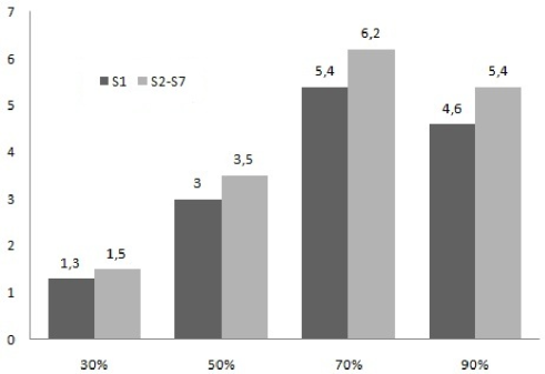
Figure 1: Average of $Impr$ for strategies S1 and S2-S7

As we have mentioned, strategies S2-S7 reached the same bound in every instance. One way to tie them is by inspecting the average of $Time$, i.e. the time elapsed, and $Cuts$, i.e. the number of cuts generated. The smaller $Time$ is, the sooner the algorithm reaches the best bound. On the other hand, the less $Cuts$ is, the better the quality of the cuts involved are. Table 2 resumes these results. Best values are emphasized with bold fond.

%Density	Time						Cuts
Graph	S2	S3	S4	S5	S6	S7	S2	S3	S4	S5	S6	S7
30	77	75	74	82	82	98	2034	2053	2053	2093	2093	3203
50	241	248	248	267	267	252	3694	3796	3796	4065	4065	3944
70	648	601	632	700	738	735	6182	5805	5670	6306	6405	6377
90	720	763	612	658	610	610	5443	5493	5065	5187	5143	5143

Table 2: Average of $Time$ and $Cuts$ for strategies S2-S7

As we can see from Table 2, strategy S4 reaches the best lower bound with fewer cuts for graphs having at least 70% of density and the amount of cuts generated is relatively acceptable for graphs having at most 50% of density. Strategy S4 also has the best balance between number of cuts generated and time consumed. Therefore, this strategy is a good candidate for our cutting-plane algorithm.

From the previous results we conclude that the cuts obtained from the polyhedral study are indeed effective. They appear to be strong in practice, increasing significantly the initial lower bound.

Nevertheless, the long-term efficiency of cuts can not be appreciated here and require further experimentation. This topic is covered in the next section.

4.4 Long-term efficiency of cuts

The purpose of the following experiment is to compare the Branch and Bound (B&B) algorithm of CPLEX with a Cut and Branch. The algorithm consists of applying 30 iterations of the cutting-plane algorithm to the initial relaxation. Then, we run a Branch and Bound enumeration until the optimal solution is found or a time limit of 2 hours is reached.

In order to do that, we apply both algorithms to 40 randomly generated graphs with different number of vertices and densities of edges. Since instances having 10% and 90% of density are easier to solve, we increased the number of vertices of them.

Preliminary experiments showed that strategies S2-S6 have a similar behaviour each other, although S4 presents the best performance among them. This led us to deepen the analysis of strategies S1, S4 and S7. Table 3 reports:

• Percentage of solved instances within 2 hours of execution.

• Average of nodes evaluated over solved instances.

• Average of total CPU time in seconds over solved instances.

Num. of	%Density	% Solved				Nodes				Time
Vertices	Graph	B&B	S1	S4	S7	B&B	S1	S4	S7	B&B	S1	S4	S7
90	10	100	100	100	100	2933	3050	1718	1718	33	33	21	21
60	30	100	100	100	100	7515	2976	1050	6567	129	52	35	130
60	50	100	100	100	100	29490	20639	21232	15786	974	1065	812	812
60	70	87.5	100	100	100	19811	12891	5330	6454	734	508	327	340
90	90	62.5	62.5	100	100	52545	35538	12645	15536	2332	2404	689	1088

Table 3: Performance of different strategies

The new inequalities show again a substantial improvement and, in particular, strategy S4 is established as the best one. It is worth mentioning that strategy S7 evaluated fewer nodes than S4 when solving instances of 50% of density, but this reduction on the number of nodes was not enough to counteract the CPU time elapsed.

From the latter results we conclude that the new inequalities used as cuts are good enough to be considered as part of the implementation of a further competitive Branch and Cut algorithm that solves the ECP.

Appendix A Introduction

In this appendix we present sufficient conditions for some valid inequalities related to the Equitable Coloring Problem to be facet-defining inequalities.

All the proofs are based in the same technique, frequently used in the literature for this kind of results, which is described in the following remark.

Remark 32.

Let $\pi^{X}x+\pi^{W}w\leq\pi_{0}$ be a valid inequality for $\mathcal{ECP}$ defining a proper face $\mathcal{F}^{\prime}$. In order to prove that $\mathcal{F}^{\prime}$ is a facet of $\mathcal{ECP}$ we have to show that, given any face $\mathcal{F}=\{(x,w)\in\mathcal{ECP}~{}:~{}\lambda^{X}x+\lambda^{W}w=\lambda_{0}\}$ such that $\mathcal{F}^{\prime}\subset\mathcal{F}$, $\lambda^{X}x+\lambda^{W}w=\lambda_{0}$ can be written as a linear combination of $\pi^{X}x+\pi^{W}w=\pi_{0}$ and the minimal equation system for $\mathcal{ECP}$ given in Theorem (4). This last condition becomes equivalent to prove that $(\lambda^{X},\lambda^{W})$ verifies an equation system of $dim(\mathcal{ECP})-1$ equalities. The validity of each equality in the system is derived from the condition $\lambda^{X}x^{1}+\lambda^{W}w^{1}=\lambda_{0}=\lambda^{X}x^{2}+\lambda^{W}w^{2}$ applied on a suitable pair of equitable colorings $(x^{1},w^{1}),(x^{2},w^{2})$ lying on $\mathcal{F}^{\prime}$.

For the sake of simplicity, we directly present the corresponding equation system on $(\lambda^{X},\lambda^{W})$ and the proposed equitable colorings used to derive each equation, bypassing how to get that equation system from the minimal equation system given in Theorem (4) and the inequality at hand.

As we have mentioned in Section 2, we present equitable colorings by using mappings, color classes or binary vectors, according to our convenience.

A.1 2-rank inequalities

Theorem 33.

Let $G$ be a monotone graph, $S\subset V$ such that $\alpha(S)=2$ and $j\leq\lceil n/2\rceil-1$. If

1. there exists a stable set $H$ of size 3 in $G$ such that:

   • if $n$ is odd, the complement of $G-H$ has a perfect matching $M$ and both endpoints of some edge of $M$ belong to $S$,

   • if $n$ is even, there exists another stable set $H^{\prime}$ of size 3 in $G$ such that $H\cap H^{\prime}=\varnothing$, the complement of $G-(H\cup H^{\prime})$ has a perfect matching $M$, both endpoints of some edge of $M$ belong to $S$ and there exist vertices $h\in H$, $h^{\prime}\in H^{\prime}$ not adjacent each other,

2. for all $v\in V\backslash S$, there exist different vertices $s,s^{\prime}\in S$ and a stable set $H_{v}=\{v,s,s^{\prime}\}$ in $G$ such that:

   • if $n$ is odd, the complement of $G-H_{v}$ has a perfect matching,

   • if $n$ is even, there exists another stable set $H^{\prime}_{v}$ of size 3 in $G$ such that $H_{v}\cap H^{\prime}_{v}=\varnothing$ and the complement of $G-(H_{v}\cup H^{\prime}_{v})$ has a perfect matching,

3. for all $k$ such that $\max\{\chi_{eq},j\}\leq k\leq\lceil n/2\rceil-2$, there exists a $k$-eqcol where two vertices of $S$ share the same color,

then the $(S,j)$-rank inequality, i.e.

$$\sum_{v\in S}x_{vj}+\sum_{v\in V}x_{vn-1}\leq 2w_{j}+w_{n-1}-w_{n},$$ (19)

defines a facet of $\mathcal{ECP}$.

Proof.

Let $\mathcal{F}^{\prime}$ be the face of $\mathcal{ECP}$ defined by (19) and $\mathcal{F}=\{(x,w)\in\mathcal{ECP}~{}:~{}\lambda^{X}x+\lambda^{W}w=\lambda_{0}\}$ be a face such that $\mathcal{F}^{\prime}\subset\mathcal{F}$. According to Remark 32, we have to prove that $(\lambda^{X},\lambda^{W})$ verifies the following equation system:

1. $\lambda^{X}_{vj}=\lambda^{X}_{vn}+\lambda^{W}_{n},~{}~{}~{}\forall~{}v\in S$.

2. $\lambda^{X}_{vn-1}=\lambda^{X}_{vn}+\lambda^{W}_{n},~{}~{}~{}\forall~{}v\in V$.

3. $\lambda^{X}_{vk}=\lambda^{X}_{vn-1}+\lambda^{W}_{n-1},~{}~{}~{}\forall~{}v\in V,~{}1\leq k\leq n-2,~{}k\neq j$.

4. $\lambda^{X}_{vj}=\lambda^{X}_{vn-1}+\lambda^{W}_{n-1},~{}~{}~{}\forall~{}v\in V\backslash S$.

5. $\lambda^{W}_{k}=0,~{}~{}~{}\forall~{}\chi_{eq}+1\leq k\leq n-2,~{}k\neq j$.

6. If $j\geq\chi_{eq}+1$ then $\lambda^{W}_{j}=-2\lambda^{W}_{n-1}$.

We present pairs of equitable colorings lying on $\mathcal{F}^{\prime}$ that allow us to prove the validity of each equation in the previous system.

1. Let $s,s^{\prime}\in S$ be non adjacent vertices.
   Case $v=s$. Let $c^{1}$ be a $(n-1)$-eqcol such that $c^{1}(s)=c^{1}(s^{\prime})=j$ and $c^{2}=intro(c^{1},s)$. Then, $\lambda^{X}_{sj}=\lambda^{X}_{sn}+\lambda^{W}_{n}$.
   Case $v\neq s$. Let $c^{1}$ be a $n$-eqcol such that $c^{1}(v)=j$, $c^{1}(s)=n$ and $c^{2}=swap_{j,n}(c^{1})$. Then, $\lambda^{X}_{vj}+\lambda^{X}_{sn}=\lambda^{X}_{vn}+\lambda^{X}_{sj}$. Since $\lambda^{X}_{sj}=\lambda^{X}_{sn}+\lambda^{W}_{n}$, we obtain $\lambda^{X}_{vj}=\lambda^{X}_{vn}+\lambda^{W}_{n}$.

2. Case $v\notin S$. By hypothesis (ii), there exist $s,s^{\prime}\in S$ such that $\{v,s,s^{\prime}\}$ is a stable set. Let $c^{1}$ be a $(n-1)$-eqcol such that $c^{1}(v)=c^{1}(s)=n-1$, $c^{1}(s^{\prime})=j$ and $c^{2}=intro(c^{1},v)$. Therefore, $\lambda^{X}_{vn-1}=\lambda^{X}_{vn}+\lambda^{W}_{n}$.
   Case $v\in S$ and $|S|=2$. By hypothesis (ii), there exist $u\in V\backslash S$ and $v^{\prime}\in S$ such that $\{u,v,v^{\prime}\}$ is a stable set. Let $c^{1}$ be a $(n-1)$-eqcol such that $c^{1}(u)=c^{1}(v)=n-1$, $c^{1}(v^{\prime})=j$ and $c^{2}=intro(c^{1},v)$. Therefore, $\lambda^{X}_{vn-1}=\lambda^{X}_{vn}+\lambda^{W}_{n}$.
   Case $v\in S$ and $|S|\geq 3$. Let $s,s^{\prime}\in S$ be non adjacent vertices, $c^{1}$ be a $(n-1)$-eqcol such that $c^{1}(s)=c^{1}(s^{\prime})=n-1$ and other vertex of $S$ is painted with color $j$, and $c^{2}=intro(c^{1},s)$. Then, $\lambda^{X}_{sn-1}=\lambda^{X}_{sn}+\lambda^{W}_{n}$ and the condition is proved for the case $v=s$. If instead $v\neq s$, let $c^{1}$ be a $n$-eqcol such that $c^{1}(v)=n-1$, $c^{1}(s)=n$, other vertex of $S$ is painted with color $j$ and $c^{2}=swap_{n,n-1}(c^{1})$. Then, $\lambda^{X}_{vn-1}+\lambda^{X}_{sn}=\lambda^{X}_{vn}+\lambda^{X}_{sn-1}$. Since $\lambda^{X}_{sn-1}=\lambda^{X}_{sn}+\lambda^{W}_{n}$, we conclude that $\lambda^{X}_{vn-1}=\lambda^{X}_{vn}+\lambda^{W}_{n}$.

3. Let $H$ and $M$ be the stable set and the matching given by hypothesis (i). Let $s,s^{\prime}\in S$ be the endpoints of an edge of $M$ and let $u,u^{\prime}\in H$.
   Case $v=u$. Let $c^{1}$ be a $(n-2)$-eqcol such that $c^{1}(u)=c^{1}(u^{\prime})=k$, $c^{1}(s)=c^{1}(s^{\prime})=j$ and $c^{2}=intro(c^{1},u)$. We conclude that $\lambda^{X}_{uk}=\lambda^{X}_{un-1}+\lambda^{W}_{n-1}$.
   Case $v\neq u$. Let $c^{1}$ be a $n$-eqcol such that $c^{1}(u)=k$, $c^{1}(v)=n-1$, a vertex of $S$ is painted with color $j$ and $c^{2}=swap_{k,n-1}(c^{1})$. Then, $\lambda^{X}_{uk}+\lambda^{X}_{vn-1}=\lambda^{X}_{un-1}+\lambda^{X}_{vk}$. Since $\lambda^{X}_{uk}=\lambda^{X}_{un-1}+\lambda^{W}_{n-1}$, we conclude that $\lambda^{X}_{vk}=\lambda^{X}_{vn-1}+\lambda^{W}_{n-1}$.

4. Let $H_{v}=\{v,s,s^{\prime}\}$, $H^{\prime}_{v}$ (if $n$ is even) and $M_{v}$ be the stable sets and the matching given by hypothesis (ii), and let $H$, $H^{\prime}$ (if $n$ is even) and $M$ be the stable sets and the matching given by hypothesis (i). Let $c^{1}$ be a $(\lceil n/2\rceil-1)$-eqcol such that the color class $j$ is $H_{v}$ and the remaining color classes are $H^{\prime}_{v}$ (if $n$ is even) and the endpoints of edges of $M_{v}$. Let $\hat{s},\hat{s}^{\prime}\in S$ be the endpoints of an edge of $M$ and let $c^{2}$ be a $(\lceil n/2\rceil-1)$-eqcol such that the color class $j$ is $\{\hat{s},\hat{s}^{\prime}\}$ and the remaining color classes are $H$, $H^{\prime}$ (if $n$ is even) and the endpoints of edges of $M$ except $(\hat{s},\hat{s}^{\prime})$. These colorings imply

   $$\lambda^{X}_{vj}+\lambda^{X}_{sj}+\lambda^{X}_{s^{\prime}j}+\sum_{w\in V\backslash\{v,s,s^{\prime}\}}\lambda^{X}_{wc^{1}(w)}=\lambda^{X}_{\hat{s}j}+\lambda^{X}_{\hat{s}^{\prime}j}+\sum_{w\in V\backslash\{\hat{s},\hat{s}^{\prime}\}}\lambda^{X}_{wc^{2}(w)}.$$

   Applying conditions (a)-(c), this last equality becomes

   $$\lambda^{X}_{vj}+\sum_{w\in V\backslash\{v\}}\lambda^{X}_{wn}+(n-3)\lambda^{W}_{n-1}+(n-1)\lambda^{W}_{n}=\sum_{w\in V}\lambda^{X}_{wn}+(n-2)\lambda^{W}_{n-1}+n\lambda^{W}_{n},$$

   giving rise to the desired result.

5. Let us observe that from any $k$-eqcol $(x^{1},w^{1})$ and any $(k-1)$-eqcol $(x^{2},w^{2})$ lying on $\mathcal{F}^{\prime}$ we get $\lambda^{X}x^{1}+\lambda^{W}_{k}=\lambda^{X}x^{2}$. Then, applying conditions (a)-(d) yields $\lambda^{W}_{k}=0$.
   Thus we only need to prove that, for any $r$ such that $\chi_{eq}\leq r\leq n-2$, there exists an $r$-eqcol $c$ lying on $\mathcal{F}^{\prime}$.
   Case $r<j$. The existence of $c$ is guaranteed by the monotonicity of $G$.
   Case $j\leq r\leq\lceil n/2\rceil-2$. Hypothesis (iii) guarantees the existence of an $r$-eqcol $c^{\prime}$ where two vertices $s,s^{\prime}\in S$ satisfy $c^{\prime}(s)=c^{\prime}(s^{\prime})$. Then, $c=swap_{c^{\prime}(s),j}(c^{\prime})$ is an $r$-eqcol that lies on $\mathcal{F}^{\prime}$.
   Case $r=\lceil n/2\rceil-1$. $c$ may be one of the colorings given in condition (d).
   Case $r=\lceil n/2\rceil$. Let $H$, $H^{\prime}$ (if $n$ is even) and $M$ be the stable sets and the matching given by hypothesis (i). Let $s,s^{\prime}\in S$ be the endpoints of an edge of $M$ and let $h\in H$, $h^{\prime}\in H^{\prime}$ (if $n$ is even) be non adjacent vertices.
   If $n$ is odd, color classes of $c$ are $\{h\}$, $H\backslash\{h\}$ and the endpoints of edges of $M$ where $\{s,s^{\prime}\}$ is the class $j$. If instead $n$ is even, color classes of $c$ are $\{h,h^{\prime}\}$, $H\backslash\{h\}$, $H^{\prime}\backslash\{h^{\prime}\}$ and the endpoints of edges of $M$ where $\{s,s^{\prime}\}$ is the class $j$.
   Case $r\geq\lceil n/2\rceil+1$. Let us consider the $\lceil n/2\rceil$-eqcol yielded in the previous case and let $v_{1},v_{2}$ be vertices sharing a color different from $j$. In order to generate a $(\lceil n/2\rceil+1)$-eqcol $c$, we introduce a new color on $v_{1}$, i.e. $c=intro(c^{\prime},v_{1})$ where $c^{\prime}$ is the $\lceil n/2\rceil$-eqcol. By repeating this procedure, we can generate a $(\lceil n/2\rceil+2)$-eqcol and so on.

6. Let $c^{1}$ be a $j$-eqcol such that $c^{1}(s)=c^{1}(s^{\prime})=j$ for some $s,s^{\prime}\in S$ and $c^{2}$ be a $(j-1)$-eqcol (the existence of these colorings is proved above). Hence,

   $$\lambda^{X}_{sj}+\lambda^{X}_{s^{\prime}j}+\sum_{v\in V\backslash\{s,s^{\prime}\}}\lambda^{X}_{vc^{1}(v)}+\lambda^{W}_{j}=\sum_{v\in V}\lambda^{X}_{vc^{2}(v)}.$$

   Application of conditions (a)-(d) yields $\lambda^{W}_{j}=-2\lambda^{W}_{n-1}$.

∎

Let us present an example where the previous theorem is applied.

Example. Let $G$ be the graph presented in Figure 2. We have that $G$ is monotone and $\chi_{eq}(G)=5$. If $S=\{1,2,\ldots,7\}$, $\alpha(S)=2$ and $H=\{4,7,8\}$ is a stable set such that $\overline{G-H}$ has the perfect matching $\{(1,10),(2,11),(3,5),(6,9)\}$ with $\{3,5\}\subset S$. Moreover, it is not hard to verify that for all $v\in\{8,9,10,11\}$ there exists a stable set $H_{v}=\{4,7,v\}$ such that $\overline{G-H_{v}}$ has a perfect matching. Then, if $1\leq j\leq 5=\lceil 11/2\rceil-1$, the $(S,j)$-rank inequality is a facet-defining inequality of $\mathcal{ECP}(G)$.

Figure 2:

Theorem 34.

Let $G$ be a monotone graph, $S\subset V$ such that $\alpha(S)=2$ and $Q=\{q\in S~{}:~{}S\subset N[q]\}$. If $|Q|\geq 2$ and

1. no connected component of the complement of $G[S\backslash Q]$ is bipartite,

2. for all $v\in V\backslash S$ verifying $Q\subset N(v)$, there exist two vertices $s,s^{\prime}\in S\backslash Q$ and a stable set $H_{v}=\{v,s,s^{\prime}\}$ in $G$ such that:

   • if $n$ is odd, the complement of $G-H_{v}$ has a perfect matching,

   • if $n$ is even, there exists another stable set $H^{\prime}_{v}$ of size 3 in $G$ such that $H_{v}\cap H^{\prime}_{v}=\varnothing$ and the complement of $G-(H_{v}\cup H^{\prime}_{v})$ has a perfect matching,

then, for all $j\leq\lceil n/2\rceil-1$, the $(S,Q,j)$-2-rank inequality, i.e.

$$\sum_{v\in S\backslash Q}x_{vj}+2\sum_{v\in Q}x_{vj}\leq 2w_{j},$$ (20)

defines a facet of $\mathcal{ECP}$.

Proof.

Let $q,q^{\prime}$ be different vertices of $Q$.

Let $\mathcal{F}^{\prime}$ be the face of $\mathcal{ECP}$ defined by (20) and $\mathcal{F}=\{(x,w)\in\mathcal{ECP}~{}:~{}\lambda^{X}x+\lambda^{W}w=\lambda_{0}\}$ be a face such that $\mathcal{F}^{\prime}\subset\mathcal{F}$. According to Remark 32, we have to prove that $(\lambda^{X},\lambda^{W})$ verifies the following equation system:

1. $\lambda^{X}_{vj}=\lambda^{X}_{vn}+\lambda^{W}_{n},~{}~{}~{}\forall~{}v\in V\backslash S~{}\textrm{such that}~{}Q\backslash N(v)\neq\varnothing$.

2. $\lambda^{X}_{vk}=\lambda^{X}_{vn}+\lambda^{W}_{n},~{}~{}~{}\forall~{}v\in V,~{}1\leq k\leq n-1,~{}k\neq j$.

3. $\lambda^{X}_{qn}+\lambda^{X}_{vj}=\lambda^{X}_{qj}+\lambda^{X}_{vn},~{}~{}~{}\forall~{}v\in Q\backslash\{q\}$.

4. $\lambda^{X}_{qn}+2\lambda^{X}_{vj}=2\lambda^{X}_{vn}+\lambda^{X}_{qj}+\lambda^{W}_{n},~{}~{}~{}\forall~{}v\in S\backslash Q$.

5. $\lambda^{X}_{vj}=\lambda^{X}_{vn}+\lambda^{W}_{n},~{}~{}~{}\forall~{}v\in V\backslash S~{}\textrm{such that}~{}Q\subset N(v)$.

6. $\lambda^{W}_{k}=0,~{}~{}~{}\forall~{}\chi_{eq}+1\leq k\leq n-1,~{}k\neq j$.

7. If $j\geq\chi_{eq}+1$ then $\lambda^{X}_{qn}+\lambda^{W}_{n}=\lambda^{X}_{qj}+\lambda^{W}_{j}$.

We present pairs of equitable colorings lying on $\mathcal{F}^{\prime}$ that allow us to prove the validity of each equation in the previous system.

1. Let $\hat{q}\in Q\backslash N(v)$ and let $c^{1}$ be a $(n-1)$-eqcol such that $c^{1}(\hat{q})=c^{1}(v)=j$ and $c^{2}=intro(c^{1},v)$. We conclude that $\lambda^{X}_{vj}=\lambda^{X}_{vn}+\lambda^{W}_{n}$.

2. Let $s,s^{\prime}\in S\backslash Q$ be non adjacent vertices.
   Case $v=s$. Let $c^{1}$ be a $(n-1)$-eqcol such that $c^{1}(s)=c^{1}(s^{\prime})=k$ and $c^{1}(q)=j$, and $c^{2}=intro(c^{1},s)$. Then, $\lambda^{X}_{sk}=\lambda^{X}_{sn}+\lambda^{W}_{n}$.
   Case $v\neq s$. Let $c^{1}$ be a $n$-eqcol such that $c^{1}(v)=k$, $c^{1}(s)=n$. If $v=q$, we make $c^{1}(q^{\prime})=j$. Otherwise, we make $c^{1}(q)=j$. From the coloring $c^{2}=swap_{k,n}(c^{1})$ we have $\lambda^{X}_{vk}+\lambda^{X}_{sn}=\lambda^{X}_{vn}+\lambda^{X}_{sk}$ and since $\lambda^{X}_{sk}=\lambda^{X}_{sn}+\lambda^{W}_{n}$ we obtain $\lambda^{X}_{vk}=\lambda^{X}_{vn}+\lambda^{W}_{n}$.

3. Let $c^{1}$ be a $n$-eqcol such that $c^{1}(q)=n$, $c^{1}(v)=j$ and $c^{2}=swap_{j,n}(c^{1})$. Therefore, $\lambda^{X}_{qn}+\lambda^{X}_{vj}=\lambda^{X}_{qj}+\lambda^{X}_{vn}$.

4. Let $J$ be the connected component in the complement of $G[S\backslash Q]$ such that $v$ is a vertex of $J$. Since $\alpha(S)=2$, $J$ does not have triangles. By hypothesis (i), $J$ is not bipartite and therefore there exists at least an odd cycle in $J$ of size $p$ with $p\geq 5$.
   Now, let $d(v)$ be the minimum distance in $J$ between $v$ and all the odd cycles in $J$, where the distance from a vertex $v$ to an odd cycle is defined as the minimum number of vertices of a path between $v$ and a vertex of the odd cycle. Condition (d) is proved by induction on $d(v)$.
   Case $d(v)=0$. Then, $v$ belongs to an odd cycle of size $p\geq 5$ in $J$. Let $v_{1}=v,v_{2},\ldots,v_{p}\in S\backslash Q$ be the vertices of that odd cycle, and let $k_{1},k_{2},\ldots,k_{p+1}$ be colors different from $j$.
   We denote by $\oplus$ the sum of two integers modulo $p$. Let $c^{1}$, $c^{2}$, $\ldots$, $c^{p}$ be $(n-1)$-eqcols such that, for each $1\leq i\leq p$, $c^{i}(v_{i})=j$, $c^{i}(v_{i\oplus 1})=j$, $c^{i}(v_{r})=k_{r}~{}~{}\forall~{}r\in\{1,\ldots,p\}\backslash\{i,i\oplus 1\}$, $c^{i}(q)=k_{p+1}$, and let $c^{p+1}$ be a $n$-eqcol such that $c^{p+1}(v_{1})=n$, $c^{p+1}(v_{r})=k_{r}~{}~{}\forall~{}r\in\{2,\ldots,p\}$, $c^{p+1}(q)=j$. For instance, if $p=5$, colors of $v_{1}$, $\ldots$, $v_{5}$ and $q$ would be:

   $c^{i}$ with $i$ odd							$c^{i}$ with $i$ even
   size	$v_{1}$	$v_{2}$	$v_{3}$	$v_{4}$	$v_{5}$	$q$	size	$v_{1}$	$v_{2}$	$v_{3}$	$v_{4}$	$v_{5}$	$q$
   $n-1$	$j$	$j$	$k_{3}$	$k_{4}$	$k_{5}$	$k_{6}$	$n-1$	$k_{1}$	$j$	$j$	$k_{4}$	$k_{5}$	$k_{6}$
   $n-1$	$k_{1}$	$k_{2}$	$j$	$j$	$k_{5}$	$k_{6}$	$n-1$	$k_{1}$	$k_{2}$	$k_{3}$	$j$	$j$	$k_{6}$
   $n-1$	$j$	$k_{2}$	$k_{3}$	$k_{4}$	$j$	$k_{6}$	$n$	$n$	$k_{2}$	$k_{3}$	$k_{4}$	$k_{5}$	$j$

   We assume that the remaining vertices have the same color in all the colorings. Thus, we obtain

   $$\sum_{\begin{subarray}{c}i=1\\ i~{}\textrm{odd}\end{subarray}}^{p+1}\sum_{v\in V}\lambda^{X}_{vc^{i}(v)}=\sum_{\begin{subarray}{c}i=1\\ i~{}\textrm{even}\end{subarray}}^{p+1}\sum_{v\in V}\lambda^{X}_{vc^{i}(v)}+\lambda^{W}_{n}.$$

   By condition (b), we get $\lambda^{X}_{qn}+2\lambda^{X}_{vj}=2\lambda^{X}_{vn}+\lambda^{X}_{qj}+\lambda^{W}_{n}$.
   Case $d(v)\geq 1$. Let $v^{\prime}\in J$ be a vertex adjacent to $v$ in $J$ such that $d(v^{\prime})=d(v)-1$. By inductive hypothesis, $\lambda^{X}_{qn}+2\lambda^{X}_{v^{\prime}j}=2\lambda^{X}_{v^{\prime}n}+\lambda^{X}_{qj}+\lambda^{W}_{n}$.
   Let $c^{1}$ be a $(n-1)$-eqcol such that $c^{1}(v)=c^{1}(v^{\prime})=j$ and $c^{1}(q)=k$, where $k\neq j$. Let $c^{2}$ be a $n$-eqcol such that $c^{2}(v)=k$, $c^{2}(v^{\prime})=n$, $c^{2}(q)=j$ and $c^{2}(i)=c^{1}(i)~{}~{}\forall~{}i\in V\backslash\{v,v^{\prime},q\}$. Hence $\lambda^{X}_{vj}+\lambda^{X}_{v^{\prime}j}+\lambda^{X}_{qk}=\lambda^{X}_{vk}+\lambda^{X}_{v^{\prime}n}+\lambda^{X}_{qj}+\lambda^{W}_{n}$. Multiplying this equality by 2, subtracting $\lambda^{X}_{qn}+2\lambda^{X}_{v^{\prime}j}=2\lambda^{X}_{v^{\prime}n}+\lambda^{X}_{qj}+\lambda^{W}_{n}$ and applying condition (b) yields $\lambda^{X}_{qn}+2\lambda^{X}_{vj}=2\lambda^{X}_{vn}+\lambda^{X}_{qj}+\lambda^{W}_{n}$.

5. By hypothesis (ii), we can establish a $(\lceil n/2\rceil-1)$-eqcol $c^{1}$ such that color class $j$ is $\{v,s,s^{\prime}\}$ where $s,s^{\prime}\in S$ (as we did in condition (d) of Theorem 33). Let $k$ be the color of $q$ in $c^{1}$ and $c^{2}=swap_{j,k}(c^{1})$. We get $\lambda^{X}_{vj}=\lambda^{X}_{vn}+\lambda^{W}_{n}$ by applying conditions (a)-(d).

6. Since $G$ is monotone, there exist a $k$-eqcol $c$ and a $(k-1)$-eqcol $c^{\prime}$. If $k<j$, we consider $c^{1}=c$ and $c^{2}=c^{\prime}$. If $k>j$, we consider $c^{1}=swap_{c(q),j}(c)$ and $c^{2}=swap_{c^{\prime}(q),j}(c^{\prime})$. Then, we apply conditions (a)-(e) to $\lambda^{X}x^{1}+\lambda^{W}_{k}=\lambda^{X}x^{2}$, where $x^{1}$ and $x^{2}$ are the binary variables representing colorings $c^{1}$ and $c^{2}$ respectively.

7. Let $c^{1}$ be a $j$-eqcol such that $c^{1}(q)=j$ and $c^{2}$ be a $(j-1)$-eqcol (the existence of these colorings is proved above). Then, we apply conditions (a)-(e) to $\lambda^{X}x^{1}+\lambda^{W}_{j}=\lambda^{X}x^{2}$, where $x^{1}$ and $x^{2}$ are the binary variables representing colorings $c^{1}$ and $c^{2}$ respectively.

∎

Theorem 34 states that, among other things, $j\leq\lceil n/2\rceil-1$ for the $(S,Q,j)$-2-rank-inequality to define a facet of $\mathcal{ECP}$. Indeed, this condition is only used in Theorem 34 for proving equations given in (e), i.e. $\lambda^{X}_{vj}=\lambda^{X}_{vn}+\lambda^{W}_{n},~{}\textrm{for all}~{}v\in V\backslash S~{}\textrm{such that}~{}Q\subset N(v)$. So, if every vertex $v\in V\backslash S$ verifies $Q\backslash N(v)\neq\varnothing$, these equations vanish from the equation system on $(\lambda^{X},\lambda^{W})$ and the inequality (20) defines a facet of $\mathcal{ECP}$ even though $j>\lceil n/2\rceil-1$. We have proved the following result.

Corollary 35.

Let $G$ be a monotone graph, $S\subset V$ such that $\alpha(S)=2$ and $Q=\{q\in S~{}:~{}S\subset N[q]\}$. If $|Q|\geq 2$, no connected component of the complement of $G[S\backslash Q]$ is bipartite and for all $v\in V\backslash S$, $Q\backslash N(v)\neq\varnothing$, then the $(S,Q,j)$-2-rank inequality defines a facet of $\mathcal{ECP}$ for all $j\leq n-1$.

Let us present an example where the previous result is applied.

Example. Let $G$ be the graph presented in Figure 2, $S=\{1,2,\ldots,7\}$ and $Q=\{1,2\}$. The $(S,Q,j)$-2-rank inequality is a facet-defining inequality of $\mathcal{ECP}(G)$ for $1\leq j\leq 10$ since the assumptions of Corollary 35 are satisfied: vertices $3,\ldots,7$ induce an odd cycle in $\overline{G}$ and for all $v\in\{8,9,10,11\}$, $Q\backslash N(v)=\{1,2\}$.

A.2 Subneighborhood inequalities

Theorem 36.

Let $G$ be a monotone graph, $u\in V$, $j\leq n-1$ such that $\lceil n/j\rceil\leq\lceil n/\chi_{eq}\rceil$ and $S\subset N(u)$ such that $S$ is not a clique of $G$ and, if $S\neq N(u)$ then $\alpha(S)\leq\lceil n/j\rceil-1$.
If

1. for all $3\leq i\leq\min\{\lceil n/j\rceil,\alpha(S)\}$, there exists a $\biggl{(}\biggl{\lceil}\dfrac{n}{i-1}\biggr{\rceil}-1\biggl{)}$-eqcol whose color class $C_{j}$ satisfies $|C_{j}\cap S|=i$,

2. for all $v\in N(u)\backslash S$, there exists an equitable coloring whose color class $C_{j}$ satisfies $|C_{j}\cap S|=\alpha(S)$ and $(C_{j}\cap N(u))\backslash S=\{v\}$,

then the $(u,j,S)$-subneighborhood inequality, i.e.

$$\gamma_{jS}x_{uj}+\sum_{v\in S}x_{vj}+\sum_{k=j+1}^{n}(\gamma_{jS}-\gamma_{kS})x_{uk}\leq\gamma_{jS}w_{j},$$ (21)

defines a facet of $\mathcal{ECP}$, where $\gamma_{kS}=\min\{\lceil n/k\rceil,\alpha(S)\}$.

Proof.

Let $\mathcal{F}^{\prime}$ be the face of $\mathcal{ECP}$ defined by (21) and $\mathcal{F}=\{(x,w)\in\mathcal{ECP}~{}:~{}\lambda^{X}x+\lambda^{W}w=\lambda_{0}\}$ be a face such that $\mathcal{F}^{\prime}\subset\mathcal{F}$. According to Remark 32, we have to prove that $(\lambda^{X},\lambda^{W})$ verifies the following equation system:

1. $\lambda^{X}_{vj}=\lambda^{X}_{vn}+\lambda^{W}_{n},~{}~{}~{}\forall~{}v\in V\backslash N[u]$.

2. $\lambda^{X}_{vk}=\lambda^{X}_{vn}+\lambda^{W}_{n},~{}~{}~{}\forall~{}v\in V\backslash\{u\},~{}1\leq k\leq n-1,~{}k\neq j$.

3. $\lambda^{X}_{vj}+\lambda^{X}_{un}=\lambda^{X}_{vn}+\lambda^{X}_{uj},~{}~{}~{}\forall~{}v\in S$.

4. $\lambda^{X}_{uk}+(\gamma_{jS}-1)\lambda^{X}_{uj}=\gamma_{jS}\lambda^{X}_{un}+\gamma_{jS}\lambda^{W}_{n},~{}~{}~{}\forall~{}1\leq k\leq j-1$.

5. $\lambda^{X}_{uk}+(\gamma_{kS}-1)\lambda^{X}_{uj}=\gamma_{kS}\lambda^{X}_{un}+\gamma_{kS}\lambda^{W}_{n},~{}~{}~{}\forall~{}j+1\leq k\leq n-1$.

6. $\lambda^{X}_{vj}=\lambda^{X}_{vn}+\lambda^{W}_{n},~{}~{}~{}\forall~{}v\in N(u)\backslash S$.

7. $\lambda^{W}_{k}=0,~{}~{}~{}\forall~{}\chi_{eq}+1\leq k\leq n-1,~{}k\neq j$.

8. If $j\geq\chi_{eq}+1$ then $\gamma_{jS}\lambda^{X}_{un}+\gamma_{jS}\lambda^{W}_{n}=\gamma_{jS}\lambda^{X}_{uj}+\lambda^{W}_{j}$.

We present pairs of equitable colorings lying on $\mathcal{F}^{\prime}$ that allow us to prove the validity of each equation in the previous system.

1. Let $c^{1}$ be a $(n-1)$-eqcol such that $c^{1}(u)=c^{1}(v)=j$ and $c^{2}=intro(c^{1},v)$. We conclude that $\lambda^{X}_{vj}=\lambda^{X}_{vn}+\lambda^{W}_{n}$.

2. Let $s,s^{\prime}\in S$ be non adjacent vertices.
   Case $v=s$. Let $c^{1}$ be a $(n-1)$-eqcol such that $c^{1}(s)=c^{1}(s^{\prime})=k$, $c^{1}(u)=j$ and $c^{2}=intro(c^{1},s)$. Then, $\lambda^{X}_{sk}=\lambda^{X}_{sn}+\lambda^{W}_{n}$.
   Case $v\neq s$. Let $c^{1}$ be a $n$-eqcol such that $c^{1}(v)=k$, $c^{1}(s)=n$, $c^{1}(u)=j$ and $c^{2}=swap_{k,n}(c^{1})$. We have $\lambda^{X}_{vk}+\lambda^{X}_{sn}=\lambda^{X}_{vn}+\lambda^{X}_{sk}$. Since $\lambda^{X}_{sk}=\lambda^{X}_{sn}+\lambda^{W}_{n}$, we conclude that $\lambda^{X}_{vk}=\lambda^{X}_{vn}+\lambda^{W}_{n}$.

3. Let $c^{1}$ be a $n$-eqcol such that $c^{1}(v)=j$, $c^{1}(u)=n$ and $c^{2}=swap_{j,n}(c^{1})$. Therefore, $\lambda^{X}_{vj}+\lambda^{X}_{un}=\lambda^{X}_{vn}+\lambda^{X}_{uj}$.

4. Case $\gamma_{jS}=2$. Let $c^{1}$ be a $(n-1)$-eqcol such that $c^{1}(u)=k$ and $c^{1}(s)=c^{1}(s^{\prime})=j$ where $s,s^{\prime}\in S$.
   Case $\gamma_{jS}\geq 3$. Let $c$ be the $(\lceil\frac{n}{\gamma_{jS}-1}\rceil-1)$-eqcol given by hypothesis (i) and $c^{1}=swap_{c(u),k}(c)$.
   In both cases, $c^{1}(u)=k$. Now, let $C_{j}$ and $C_{k}$ be the color classes $j$ and $k$ of $c^{1}$ respectively. Considering $c^{2}=swap_{j,k}(c^{1})$ give rise to

   $$\lambda^{X}_{uk}+\sum_{v\in C_{j}}\lambda^{X}_{vj}+\sum_{v\in C_{k}\backslash\{u\}}\lambda^{X}_{vk}=\lambda^{X}_{uj}+\sum_{v\in C_{j}}\lambda^{X}_{vk}+\sum_{v\in C_{k}\backslash\{u\}}\lambda^{X}_{vj}.$$

   Since $|C_{j}\cap S|=\gamma_{jS}$, we have $C_{j}\subset S$ and we can apply (a)-(c) in order to get $\lambda^{X}_{uk}+(\gamma_{jS}-1)\lambda^{X}_{uj}=\gamma_{jS}\lambda^{X}_{un}+\gamma_{jS}\lambda^{W}_{n}$.

5. We proceed in the same way as in (d) except that, for the case $\gamma_{jS}\geq 3$, we use the $(\lceil\frac{n}{\gamma_{kS}-1}\rceil-1)$-eqcol given by hypothesis (i) instead of the $(\lceil\frac{n}{\gamma_{jS}-1}\rceil-1)$-eqcol.

6. In first place, let us note that $v\in N(u)\backslash S$ implies $S\subsetneqq N(u)$. Then, $\alpha(S)\leq\lceil n/j\rceil-1$ and, by hypothesis (ii), there exists a coloring $c^{1}$ that paints $v$ and $\alpha(S)$ vertices of $S$ with color $j$ but the remaining vertices of $N(u)$ do not use $j$. Let $k$ be the color used by vertex $u$ in $c^{1}$ and let $C_{j}$, $C_{k}$ be the color classes $j$ and $k$ in $c^{1}$ respectively, and $c^{2}=swap_{j,k}(c^{1})$. We have

   $$\lambda^{X}_{uk}+\lambda^{X}_{vj}+\sum_{w\in C_{j}\backslash\{v\}}\lambda^{X}_{wj}+\sum_{w\in C_{k}\backslash\{u\}}\lambda^{X}_{wk}=\lambda^{X}_{uj}+\lambda^{X}_{vk}+\sum_{w\in C_{j}\backslash\{v\}}\lambda^{X}_{wk}+\sum_{w\in C_{k}\backslash\{u\}}\lambda^{X}_{wj}.$$

   In virtue of conditions (a)-(e), we obtain $\lambda^{X}_{vj}=\lambda^{X}_{vn}+\lambda^{W}_{n}$.

7. Since $G$ is monotone, there exist a $k$-eqcol $c$ and a $(k-1)$-eqcol $c^{\prime}$. If $k<j$, we consider $c^{1}=c$ and $c^{2}=c^{\prime}$. If $k>j$, we consider $c^{1}=swap_{c(u),j}(c)$ and $c^{2}=swap_{c^{\prime}(u),j}(c^{\prime})$. Then, we apply conditions (a)-(f) to $\lambda^{X}x^{1}+\lambda^{W}_{k}=\lambda^{X}x^{2}$, where $x^{1}$ and $x^{2}$ are the binary variables representing colorings $c^{1}$ and $c^{2}$ respectively.

8. Let $c^{1}$ be a $j$-eqcol such that $c^{1}(u)=j$ and $c^{2}$ be a $(j-1)$-eqcol (the existence of these colorings is proved above). Then, we apply conditions (a)-(f) to $\lambda^{X}x^{1}+\lambda^{W}_{j}=\lambda^{X}x^{2}$, where $x^{1}$ and $x^{2}$ are the binary variables representing colorings $c^{1}$ and $c^{2}$ respectively.

∎

Let us present two examples where the previous theorem is applied.

Example. Let $G$ be the graph given in Figure 3(a). We have that $G$ is monotone and $\chi_{eq}(G)=3$. Let us consider $u=1$, $S=N(1)$ and $j=3$. In order to prove that the $(u,j,S)$-subneighborhood inequality defines a facet of $\mathcal{ECP}(G)$, it is enough to exhibit a ($\lceil\frac{11}{2}\rceil-1$)-eqcol such that $|C_{3}\cap S|=3$ and a ($\lceil\frac{11}{3}\rceil-1$)-eqcol such that $|C_{3}\cap S|=4$. Both colorings are shown in Figure 3 (b) and (c) respectively.

It is not hard to see that the $(u,j,S)$-subneighborhood inequality is also facet-defining for $4\leq j\leq 10$. On the other hand, $(u,j,S)$-subneighborhood inequality with $j\in\{1,2\}$ is facet-defining by Theorem 16.

Therefore, the $(u,j,S)$-subneighborhood inequality defines a facet of $\mathcal{ECP}(G)$ for all $1\leq j\leq 10$.

Example. Let us consider again the graph given in Figure 3(a). The $(u,j,S)$-subneighborhood inequality with $u=1$, $j=3$ and $S=\{3,4,5\}$ is facet-defining since $\alpha(S)\leq\lceil\frac{11}{3}\rceil-1$ and there exist the following colorings: a ($\lceil\frac{11}{2}\rceil-1$)-eqcol such that $|C_{3}\cap S|=3$, an equitable coloring such that $|C_{3}\cap S|=3$ and $(C_{3}\cap N(1))\backslash S=\{2\}$, and an equitable coloring such that $|C_{3}\cap S|=3$ and $(C_{3}\cap N(1))\backslash S=\{6\}$. These colorings are shown in Figure 3 (b), (c) and (d) respectively.

Figure 3:

Corollary 37.

Let $G$ be a monotone graph, $j\leq n-1$ and $q\in V$ such that $\alpha(N(q))=2$. Then, the $(q,j,N(q))$-subneighborhood inequality defines a facet of $\mathcal{ECP}$.
Moreover, let $S\subset V$ with $\alpha(S)=2$ and $S\subsetneqq N(q)$. If $j\leq\lceil n/2\rceil-1$ and for all $v\in N(q)\backslash S$, there exist different vertices $s,s^{\prime}\in S$ and a stable set $H_{v}=\{v,s,s^{\prime}\}$ in $G$ such that:

• If $n$ is odd, the complement of $G-H_{v}$ has a perfect matching,

• If $n$ is even, there exists another stable set $H^{\prime}_{v}$ of size 3 in $G$ such that $H_{v}\cap H^{\prime}_{v}=\varnothing$ and the complement of $G-(H_{v}\cup H^{\prime}_{v})$ has a perfect matching,

then the $(q,j,S)$-subneighborhood inequality defines a facet of $\mathcal{ECP}$.

Proof.

Case $\lceil n/j\rceil\leq\lceil n/\chi_{eq}\rceil$. The $(q,j,N(q))$-subneighborhood inequality defines a facet of $\mathcal{ECP}$ since hypotheses (i) and (ii) from Theorem 36 hold trivially.
Now, let us consider the $(q,j,S)$-subneighborhood inequality. Since $j\leq\lceil n/2\rceil-1$, we have that $\alpha(S)=2\leq\lceil n/j\rceil-1$. Moreover, hypothesis (i) from Theorem 36 holds trivially.
Let $v\in N(q)\backslash S$ and $M_{v}$, $H_{v}=\{v,s,s^{\prime}\}$ and $H^{\prime}_{v}$ (if $n$ is even) be the matching and the stable sets given by the hypothesis. Consider the $(\lceil n/2\rceil-1)$-eqcol such that the color class $C_{j}$ is $H_{v}$ and the remaining color classes are $H^{\prime}_{v}$ (if $n$ is even) and the endpoints of edges of $M_{v}$. Then, $|C_{j}\cap S|=2$, $(C_{j}\cap N(q))\backslash S=\{v\}$ and hypothesis (ii) from Theorem 36 holds. Therefore, the $(q,j,S)$-subneighborhood inequality defines a facet of $\mathcal{ECP}$.
Case $\lceil n/j\rceil>\lceil n/\chi_{eq}\rceil$. In virtue of the previous case, we know that the $(q,\chi_{eq},N(q))$-subneighborhood and the $(q,\chi_{eq},S)$-subneighborhood are facet-defining inequalities of $\mathcal{ECP}$. Hence, the $(q,j,N(q))$-subneighborhood and the $(q,j,S)$-subneighborhood inequality define facets of $\mathcal{ECP}$ due to Theorem 16. ∎

A.3 Outside-neighborhood inequalities

Theorem 38.

Let $G$ be a monotone graph, $u\in V$ such that $N(u)$ is not a clique and $\chi_{eq}\leq j\leq\lfloor n/2\rfloor$. If

1. there exists $\hat{v}\in V\backslash N[u]$ not universal in $G-u$,

2. if $n$ is odd, the complement of $G-u$ has a perfect matching,

3. for all $v\in V\backslash N[u]$, the following conditions hold:

   • if $n$ is even, the complement of $G-\{u,v\}$ has a perfect matching,

   • if $n$ is odd, there exists a stable set $H_{v}\subset V\backslash\{u,v\}$ of size 3 such that the complement of $G-(H_{v}\cup\{u,v\})$ has a perfect matching,

4. for all $r$ such that $j\leq r\leq\lfloor n/2\rfloor$, we have the following:

   • if $\biggl{\lfloor}\dfrac{n}{r}\biggr{\rfloor}>\biggl{\lfloor}\dfrac{n}{r+1}\biggr{\rfloor}$, then there exists an $r$-eqcol such that $C_{j}\subset N(u)$ and an $r$-eqcol such that $u\in C_{j}$ and $|C_{j}|=\lfloor n/r\rfloor$,

   • if $\biggl{\lfloor}\dfrac{n}{r}\biggr{\rfloor}=\biggl{\lfloor}\dfrac{n}{r+1}\biggr{\rfloor}$, then there exists an $r$-eqcol satisfying conditions given in Remark 20, i.e. lying on the face defined by (22),

then the $(u,j)$-outside-neighborhood inequality, i.e.

$$\biggl{(}\biggl{\lfloor}\dfrac{n}{j}\biggr{\rfloor}-1\biggr{)}x_{uj}-\sum_{v\in V\backslash N[u]}x_{vj}+\sum_{k=j+1}^{n}b_{jk}x_{uk}\leq\sum_{k=j+1}^{n}b_{jk}(w_{k}-w_{k+1}),$$ (22)

defines a facet of $\mathcal{ECP}$, where $b_{jk}=\lfloor n/j\rfloor-\lfloor n/k\rfloor$.

Proof.

Let $\mathcal{F}^{\prime}$ be the face of $\mathcal{ECP}$ defined by (22) and $\mathcal{F}=\{(x,w)\in\mathcal{ECP}~{}:~{}\lambda^{X}x+\lambda^{W}w=\lambda_{0}\}$ be a face such that $\mathcal{F}^{\prime}\subset\mathcal{F}$. According to Remark 32, we have to prove that $(\lambda^{X},\lambda^{W})$ verifies the following equation system:

1. $\lambda^{X}_{vk}=\lambda^{X}_{vn}+\lambda^{W}_{n},~{}~{}~{}\forall~{}v\in V\backslash N[u],~{}1\leq k\leq n-1,~{}k\neq j$.

2. $\lambda^{X}_{vk}=\lambda^{X}_{vn}+\lambda^{W}_{n},~{}~{}~{}\forall~{}v\in N(u),~{}1\leq k\leq n-1$.

3. $\lambda^{X}_{uj}=\lambda^{X}_{un}+\lambda^{W}_{n}$.

4. $\lambda^{X}_{vj}=\lambda^{X}_{vn}+\lambda^{W}_{n}+\lambda^{W}_{\lfloor n/2\rfloor+1},~{}~{}~{}\forall~{}v\in V\backslash N[u]$.

5. $\lambda^{X}_{uk}=\lambda^{X}_{un}+\lambda^{W}_{n}+(\lfloor n/j\rfloor-1)\lambda^{W}_{\lfloor n/2\rfloor+1},~{}~{}~{}\forall~{}1\leq k\leq j-1$.

6. $\lambda^{X}_{uk}=\lambda^{X}_{un}+\lambda^{W}_{n}+(\lfloor n/k\rfloor-1)\lambda^{W}_{\lfloor n/2\rfloor+1},~{}~{}~{}\forall~{}j+1\leq k\leq n-1$.

7. If $j\neq\chi_{eq}$, then $\lambda^{W}_{k}=0,~{}~{}~{}\forall~{}\chi_{eq}+1\leq k\leq j$.

8. $\lambda^{W}_{k}=\biggl{(}\biggl{\lfloor}\dfrac{n}{k-1}\biggr{\rfloor}-\biggl{\lfloor}\dfrac{n}{k}\biggr{\rfloor}\biggr{)}\lambda^{W}_{\lfloor n/2\rfloor+1},~{}~{}~{}\forall~{}j+1\leq k\leq n-1,~{}k\neq\lfloor n/2\rfloor+1$.

We present pairs of equitable colorings lying on $\mathcal{F}^{\prime}$ that allow us to prove the validity of each equation in the previous system.

1. By hypothesis (i), there exist $\hat{v}\in V\backslash N[u]$ and $\hat{v}^{\prime}\in V\backslash\{u,\hat{v}\}$ not adjacent to $\hat{v}$.
   Case $v=\hat{v}$. Let $c^{1}$ be a $(n-1)$-eqcol such that $c^{1}(u)=j$, $c^{1}(\hat{v})=c^{1}(\hat{v}^{\prime})=k$ and $c^{2}=intro(c^{1},\hat{v})$. Then, $\lambda^{X}_{\hat{v}k}=\lambda^{X}_{\hat{v}n}+\lambda^{W}_{n}$.
   Case $v\neq\hat{v}$. Let $c^{1}$ be a $n$-eqcol such that $c^{1}(u)=j$, $c^{1}(v)=k$, $c^{1}(\hat{v})=n$ and $c^{2}=swap_{k,n}(c^{1})$. We have $\lambda^{X}_{vk}+\lambda^{X}_{\hat{v}n}=\lambda^{X}_{vn}+\lambda^{X}_{\hat{v}k}$ and therefore $\lambda^{X}_{vk}=\lambda^{X}_{vn}+\lambda^{W}_{n}$.

2. Let $u_{1},u_{2}\in N(u)$ be non adjacent vertices.
   Case $v=u_{1}$. Let $c^{1}$ be a $(n-1)$-eqcol such that $c^{1}(u_{1})=c^{1}(u_{2})=k$. If $k=j$ we set $c^{1}(u)=n-1$, otherwise $c^{1}(u)=j$. Let $c^{2}=intro(c^{1},u_{1})$. Then, $\lambda^{X}_{u_{1}k}=\lambda^{X}_{u_{1}n}+\lambda^{W}_{n}$.
   Case $v\neq u_{1}$. Let $c^{1}$ be a $n$-eqcol such that $c^{1}(v)=k$ and $c^{1}(u_{1})=n$. If $k=j$ we set $c^{1}(u)=n-1$, otherwise $c^{1}(u)=j$. Let $c^{2}=swap_{k,n}(c^{1})$. We have $\lambda^{X}_{vk}+\lambda^{X}_{u_{1}n}=\lambda^{X}_{vn}+\lambda^{X}_{u_{1}k}$ and therefore $\lambda^{X}_{vk}=\lambda^{X}_{vn}+\lambda^{W}_{n}$.

3. Let $v\in N(u)$, $c^{1}$ be a $n$-eqcol such that $c^{1}(u)=j$, $c^{1}(v)=n$ and $c^{2}=swap_{j,n}(c^{1})$. In virtue of condition (b), we obtain $\lambda^{X}_{uj}=\lambda^{X}_{un}+\lambda^{W}_{n}$.

4. Case $n$ even. Let $M_{v}$ be the matching given by hypothesis (iii). Let $c^{1}$ be the $\lfloor n/2\rfloor$-eqcol whose color classes are the endpoints of $M_{v}$ and $C_{j}=\{u,v\}$. Let $c^{2}=intro(c^{1},v)$. We deduce that $\lambda^{X}_{vj}=\lambda^{X}_{v\lfloor n/2\rfloor+1}+\lambda^{W}_{\lfloor n/2\rfloor+1}=\lambda^{X}_{vn}+\lambda^{W}_{n}+\lambda^{W}_{\lfloor n/2\rfloor+1}$.
   Case $n$ odd. Let $M_{v}$ and $H_{v}$ be the matching and the stable set given by hypothesis (iii). Let $c^{1}$ be the $\lfloor n/2\rfloor$-eqcol whose color classes are $H_{v}$, the endpoints of $M_{v}$ and $C_{j}=\{u,v\}$. Now, let $M$ be the matching given by hypothesis (ii) and let $v^{\prime}$ be a vertex such that $(v,v^{\prime})$ belongs to $M$. Let $c^{2}$ be the $(\lfloor n/2\rfloor+1)$-eqcol whose color classes are the endpoints of $M\backslash(v,v^{\prime})$, $C_{j}=\{u\}$ and $C_{\lfloor n/2\rfloor+1}=\{v,v^{\prime}\}$. Thus,

   $$\lambda^{X}_{vj}+\sum_{i\in V\backslash\{u,v\}}\lambda^{X}_{ic^{1}(i)}=\lambda^{X}_{v\lfloor n/2\rfloor+1}+\sum_{i\in V\backslash\{u,v\}}\lambda^{X}_{ic^{2}(i)}+\lambda^{W}_{\lfloor n/2\rfloor+1}.$$

   Conditions (a) and (b) allow us to reach the desired result.

5. Let us notice that, if $r=\lfloor n/\lfloor n/j\rfloor\rfloor$ then $\lfloor n/j\rfloor=\lfloor n/r\rfloor$, $j\leq r\leq\lfloor n/2\rfloor$ and $\lfloor\frac{n}{r}\rfloor>\lfloor\frac{n}{r+1}\rfloor$. By hypothesis (iv), there exists an $r$-eqcol $c$ such that $N(u)$ contains all the vertices painted with color $j$. Let $c^{1}=swap_{c(u),k}(c)$ and $c^{2}$ be the $r$-eqcol that paints vertex $u$ and $\lfloor n/j\rfloor-1$ vertices of $V\backslash N[u]$ with color $j$ also given by hypothesis (iv). By condition (c), we have $\lambda^{X}_{uk}+\sum_{v\in V\backslash\{u\}}\lambda^{X}_{vc^{1}(v)}=\lambda^{X}_{un}+\lambda^{W}_{n}+\sum_{v\in V\backslash\{u\}}\lambda^{X}_{vc^{2}(v)}$. Applying conditions (a), (b) and (d), we get $\lambda^{X}_{uk}=\lambda^{X}_{un}+\lambda^{W}_{n}+(\lfloor n/j\rfloor-1)\lambda^{W}_{\lfloor n/2\rfloor+1}$.

6. Case $k\leq\lfloor n/2\rfloor$. We proceed in the same way as in (e), but using $r=\lfloor n/\lfloor n/k\rfloor\rfloor$ instead of $\lfloor n/\lfloor n/j\rfloor\rfloor$.
   Case $k\geq\lfloor n/2\rfloor+1$. Then, $\lfloor n/k\rfloor=1$. Let $v\in N(u)$, $c^{1}$ be a $n$-eqcol such that $c^{1}(u)=k$, $c^{1}(v)=j$ and $c^{2}=swap_{k,j}(c^{1})$. Conditions (b) and (c) allow us to obtain $\lambda^{X}_{uk}=\lambda^{X}_{un}+\lambda^{W}_{n}$.

7. This condition can be verified by providing a $k$-eqcol $(x^{1},w^{1})$ and a $(k-1)$-eqcol $(x^{2},w^{2})$ lying on $\mathcal{F}^{\prime}$ and applying conditions (a)-(f) to equation $\lambda^{X}x^{1}+\lambda^{W}_{k}=\lambda^{X}x^{2}$.
   Thus, we only need to prove that, for any $\chi_{eq}\leq r\leq n-1$, there exists an $r$-eqcol $c$ lying on $\mathcal{F}^{\prime}$ .
   Case $r<j$. The existence of $c$ is guaranteed by the monotonicity of G.
   Case $j\leq r\leq\lfloor n/2\rfloor$. The existence of $c$ is guaranteed by hypothesis (iv).
   Case $r=\lfloor n/2\rfloor+1$. $c$ may be the $(\lfloor n/2\rfloor+1)$-eqcol yielded by condition (d).
   Case $\lfloor n/2\rfloor+2\leq r\leq n-1$. Let us consider the $(\lfloor n/2\rfloor+1)$-eqcol yielded in the previous case and let $v_{1},v_{2}$ be vertices sharing a color different from $j$. In order to generate a $(\lfloor n/2\rfloor+2)$-eqcol $c$, we introduce a new color on $v_{1}$, i.e. $c=intro(c^{\prime},v_{1})$ where $c^{\prime}$ is the $(\lfloor n/2\rfloor+1)$-eqcol. By repeating this procedure, we can generate a $(\lfloor n/2\rfloor+3)$-eqcol and so on.

∎

Let us present an example where the previous theorem is applied.

Example. Let $G$ be the graph given in Figure 3(a). Let us recall that $G$ is monotone and $\chi_{eq}(G)=3$. We apply Theorem 38 considering $u=1$ and $j=3$. It is not hard to see that the assumptions of this theorem are satisfied. Below, we present some examples of colorings related to hypothesis (iv) of Theorem 38. Figure 4(a) shows a 3-eqcol of $G$ such that $C_{3}\subset N(1)$ and Figure 4(b) shows a 3-eqcol of $G$ such that $1\in C_{3}$ and $|C_{3}|=3$.

By Theorem 23, $(1,j)$-outside-neighborhood inequalities with $j\in\{1,2\}$ are also facet-defining.

Figure 4:

A.4 Clique-neighborhood inequalities

Theorem 39.

Let $G$ be a monotone graph, $u\in V$, $Q$ be a clique of $G$ such that $Q\cap N[u]=\varnothing$ and $j,k$ be numbers verifying $3\leq k\leq\min\{\alpha(N(u))+1,\lceil n/\chi_{eq}\rceil\}$ and $1\leq j\leq\biggl{\lceil}\dfrac{n}{k-1}\biggr{\rceil}-1$. If

1. for all $v\in V\backslash(N[u]\cup Q)$, there exist $\lceil n/3\rceil\leq r\leq\lceil n/2\rceil-1$, $q_{1},q_{2}\in V$ and two $r$-eqcols such that in one of them $C_{j}=\{u,v,q_{1}\}$ and in the other $C_{j}=\{u,q_{2}\}$ ($q_{1}$ and $q_{2}$ may be the same vertex),

2. for all $t$ such that $max\{j,\chi_{eq}\}\leq t\leq n-3$, we have the following:

   • if $\biggl{\lceil}\dfrac{n}{t}\biggr{\rceil}>\biggl{\lceil}\dfrac{n}{t+1}\biggr{\rceil}$, there exist $q\in Q$ and a $t$-eqcol such that $C_{j}\subset N(u)$, $|C_{j}|=\lceil n/t\rceil$ and $u,q\in C_{t}$,

   • if $\biggl{\lceil}\dfrac{n}{t}\biggr{\rceil}=\biggl{\lceil}\dfrac{n}{t+1}\biggr{\rceil}$, there exists a $t$-eqcol satisfying conditions given in Remark 26, i.e. lying on the face defined by (23),

then the $(u,j,k,Q)$-clique-neighborhood inequality, i.e.

$$(k-1)x_{uj}+\sum_{l=\lceil\frac{n}{k-1}\rceil}^{n-2}\biggl{(}k-\biggl{\lceil}\dfrac{n}{l}\biggr{\rceil}\biggr{)}x_{ul}+(k-1)\bigl{(}x_{un-1}+x_{un}\bigr{)}+\!\!\!\sum_{v\in N(u)\cup Q}\!\!\!x_{vj}\\ +\sum_{v\in V\backslash\{u\}}\!\!\!(x_{vn-1}+x_{vn})\leq\sum_{l=j}^{n}b_{ul}(w_{l}-w_{l+1}),$$ (23)

defines a facet of $\mathcal{ECP}$, where

$$b_{ul}=\begin{cases}\min\{\lceil n/l\rceil,\alpha(N(u))+1\},&\textrm{if $j\leq l\leq\lceil n/k\rceil-1$}\\ k,&\textrm{if $\lceil n/k\rceil\leq l\leq n-2$}\\ k+1,&\textrm{if $l\geq n-1$}\end{cases}$$

Proof.

Let $\mathcal{F}^{\prime}$ be the face of $\mathcal{ECP}$ defined by (23) and $\mathcal{F}=\{(x,w)\in\mathcal{ECP}~{}:~{}\lambda^{X}x+\lambda^{W}w=\lambda_{0}\}$ be a face such that $\mathcal{F}^{\prime}\subset\mathcal{F}$. According to Remark 32, we have to prove that $(\lambda^{X},\lambda^{W})$ verifies the following equation system:

1. $\lambda^{X}_{uj}=\lambda^{X}_{un}+\lambda^{W}_{n}$.

2. $\lambda^{X}_{vn-1}=\lambda^{X}_{vn}+\lambda^{W}_{n},~{}~{}~{}\forall~{}v\in V$.

3. $\lambda^{X}_{vr}=\lambda^{X}_{vn-1}+\lambda^{W}_{n-1},~{}~{}~{}\forall~{}v\in V\backslash\{u\},~{}1\leq r\leq n-2,~{}r\neq j$.

4. $\lambda^{X}_{vj}=\lambda^{X}_{vn}+\lambda^{W}_{n},~{}~{}~{}\forall~{}v\in N(u)\cup Q$.

5. $\lambda^{X}_{vj}=\lambda^{X}_{vn-1}+\lambda^{W}_{n-1},~{}~{}~{}\forall~{}v\in V\backslash(N[u]\cup Q)$.

6. $\lambda^{X}_{ur}=\lambda^{X}_{un}+(k-1)\lambda^{W}_{n-1}+\lambda^{W}_{n},~{}~{}~{}\forall~{}1\leq r\leq\lceil\frac{n}{k-1}\rceil-1,~{}r\neq j$.

7. $\lambda^{X}_{ur}=\lambda^{X}_{un}+(\lceil n/r\rceil-1)\lambda^{W}_{n-1}+\lambda^{W}_{n},~{}~{}~{}\forall~{}\lceil\frac{n}{k-1}\rceil\leq r\leq n-2$.

8. $\lambda^{W}_{r}=(b_{ur}-b_{ur-1})\lambda^{W}_{n-1},~{}~{}~{}\forall~{}\chi_{eq}+1\leq r\leq n-2$.

We present pairs of equitable colorings lying on $\mathcal{F}^{\prime}$ that allow us to prove the validity of each equation in the previous system.

1. Let $q\in Q$, $c^{1}$ be a $(n-1)$-eqcol such that $c^{1}(u)=c^{1}(q)=j$ and $c^{2}=intro(c^{1},u)$. Then, $\lambda^{X}_{uj}=\lambda^{X}_{un}+\lambda^{W}_{n}$.

2. Case $v=u$. Let $q\in Q$, $w\in N(u)\cup Q\backslash\{q\}$, $c^{1}$ be a $(n-1)$-eqcol such that $c^{1}(u)=c^{1}(q)=n-1$, $c^{1}(w)=j$ and $c^{2}=intro(c^{1},u)$. Then, $\lambda^{X}_{un-1}=\lambda^{X}_{un}+\lambda^{W}_{n}$.
   Now, let $v_{1},v_{2}\in N(u)$ be non adjacent vertices.
   Case $v=v_{1}$. Let $c^{1}$ be a $(n-1)$-eqcol such that $c^{1}(v_{1})=c^{1}(v_{2})=n-1$, $c^{1}(u)=j$ and $c^{2}=intro(c^{1},v_{1})$. We have $\lambda^{X}_{v_{1}n-1}=\lambda^{X}_{v_{1}n}+\lambda^{W}_{n}$.
   Case $v\in V\backslash\{u,v_{1}\}$. Let $c^{1}$ be a $n$-eqcol such that $c^{1}(u)=j$, $c^{1}(v)=n-1$, $c^{1}(v_{1})=n$ and $c^{2}=swap_{n-1,n}(c^{1})$. We have $\lambda^{X}_{vn-1}+\lambda^{X}_{v_{1}n}=\lambda^{X}_{vn}+\lambda^{X}_{v_{1}n-1}$ and, since $\lambda^{X}_{v_{1}n-1}=\lambda^{X}_{v_{1}n}+\lambda^{W}_{n}$, we obtain $\lambda^{X}_{vn-1}=\lambda^{X}_{vn}+\lambda^{W}_{n}$.

3. Let $v_{1},v_{2}\in N(u)$ be non adjacent vertices and $q\in Q$.
   Case $v=v_{1}$. Let $c^{1}$ be a $(n-2)$-eqcol such that $c^{1}(v_{1})=c^{1}(v_{2})=r$, $c^{1}(u)=c^{1}(q)=j$ and $c^{2}=intro(c^{1},v_{1})$. Then, $\lambda^{X}_{v_{1}r}=\lambda^{X}_{v_{1}n-1}+\lambda^{W}_{n-1}$.
   Case $v\neq v_{1}$. Let $c^{1}$ be a $n$-eqcol such that $c^{1}(u)=j$, $c^{1}(v)=r$, $c^{1}(v_{1})=n-1$ and $c^{2}=swap_{r,n-1}(c^{1})$. We have $\lambda^{X}_{vr}+\lambda^{X}_{v_{1}n-1}=\lambda^{X}_{vn-1}+\lambda^{X}_{v_{1}r}$ and, since $\lambda^{X}_{v_{1}r}=\lambda^{X}_{v_{1}n-1}+\lambda^{W}_{n-1}$, we obtain $\lambda^{X}_{vr}=\lambda^{X}_{vn-1}+\lambda^{W}_{n-1}$.

4. Let $q\in Q$.
   Case $v=q$. Let $c^{1}$ be a $(n-1)$-eqcol such that $c^{1}(u)=c^{1}(q)=j$ and $c^{2}=intro(c^{1},q)$. Then, $\lambda^{X}_{qj}=\lambda^{X}_{qn}+\lambda^{W}_{n}$.
   Case $v\neq q$. Let $c^{1}$ be a $n$-eqcol such that $c^{1}(u)=n-1$, $c^{1}(q)=n$, $c^{1}(v)=j$ and $c^{2}=swap_{j,n}(c^{1})$. We have $\lambda^{X}_{vj}+\lambda^{X}_{qn}=\lambda^{X}_{vn}+\lambda^{X}_{qj}$ and, since $\lambda^{X}_{qj}=\lambda^{X}_{qn}+\lambda^{W}_{n}$, we obtain $\lambda^{X}_{vj}=\lambda^{X}_{vn}+\lambda^{W}_{n}$.

5. Hypothesis (i) ensures that there exists an equitable coloring $c^{1}$ such that $c^{1}(u)=c^{1}(v)=c^{1}(q_{1})=j$ and the remaining vertices do not use color $j$, and there exists another equitable coloring $c^{2}$ (with the same number of colors) such that $c^{2}(u)=c^{2}(q_{2})=j$ and the remaining vertices do not use color $j$, where $q_{1},q_{2}\in Q$. We have

   $$\sum_{w\in V\backslash\{u,v,q_{1}\}}\lambda^{X}_{wc^{1}(w)}+\lambda^{X}_{q_{1}j}+\lambda^{X}_{vj}=\sum_{w\in V\backslash\{u,v,q_{2}\}}\lambda^{X}_{wc^{2}(w)}+\lambda^{X}_{q_{2}j}+\lambda^{X}_{vc^{2}(v)}$$

   and, by conditions (b)-(d), we derive $\lambda^{X}_{vj}=\lambda^{X}_{vc^{2}(v)}=\lambda^{X}_{vn}+\lambda^{W}_{n-1}$.

6. Let $t=\lceil\frac{n}{k-1}\rceil-1$. Clearly, $max\{j,\chi_{eq}\}\leq t\leq n-3$ and $\lceil\frac{n}{t}\rceil>\lceil\frac{n}{t+1}\rceil$. By hypothesis (ii), there exists a $t$-eqcol $c$ whose class color $C_{j}$ satisfies $C_{j}\subset N(u)$ and $|C_{j}|=\lceil n/t\rceil$ and $u$ and a vertex of $Q$ use color $t$. Let $c^{1}=swap_{j,t}(c)$ and $c^{2}=swap_{r,t}(c)$ (since $t\geq j$ and $t\geq r$, both colorings are well-defined). Hence, $c^{1}(u)=j$ and $c^{2}(u)=r$. We apply conditions proved before to $\lambda^{X}x^{1}=\lambda^{X}x^{2}$, where $x^{1}$ and $x^{2}$ are the binary variables representing colorings $c^{1}$ and $c^{2}$ respectively, and we conclude that $\lambda^{X}_{ur}=\lambda^{X}_{un}+(k-1)\lambda^{W}_{n-1}+\lambda^{W}_{n}$.

7. Case $r\leq\lceil\frac{n}{2}\rceil-1$. We proceed in the same way as in (f), but using $t=\lceil\frac{n}{\lceil n/r\rceil-1}\rceil-1$ instead of $\lceil\frac{n}{k-1}\rceil-1$.
   Case $r\geq\lceil\frac{n}{2}\rceil$. Let $v_{1},v_{2}\in N(u)$ be non adjacent vertices and $q\in Q$. Let $c^{1}$ be a $(n-2)$-eqcol such that $c^{1}(v_{1})=c^{1}(v_{2})=r$, $c^{1}(u)=c^{1}(q)=j$ and $c^{2}=swap_{j,r}(c^{1})$. We apply conditions proved before to $\lambda^{X}x^{1}=\lambda^{X}x^{2}$, where $x^{1}$ and $x^{2}$ are the binary variables representing colorings $c^{1}$ and $c^{2}$ respectively, and we conclude that $\lambda^{X}_{ur}=\lambda^{X}_{un}+\lambda^{W}_{n-1}+\lambda^{W}_{n}$.

8. This condition can be verified by providing an $r$-eqcol $(x^{1},w^{1})$ and an $(r-1)$-eqcol $(x^{2},w^{2})$ lying on $\mathcal{F}^{\prime}$ and applying conditions (a)-(g) to equation $\lambda^{X}x^{1}+\lambda^{W}_{r}=\lambda^{X}x^{2}$.
   Thus, we only need to prove that, for any $\chi_{eq}\leq t\leq n-2$, there exists a $t$-eqcol $c$ lying on $\mathcal{F}^{\prime}$ .
   Case $t<j$. The existence of $c$ is guaranteed by the monotonicity of G.
   Case $j\leq t\leq n-3$. The existence of $c$ is guaranteed by hypothesis (ii).
   Case $t=n-2$. $c$ may be the $(n-2)$-eqcol yielded by condition (c).

∎

Corollary 40.

Let $G$ be a monotone graph and let $u$, $j$, $k$, $Q$ be defined as in Theorem 39. If hypothesis (ii) of Theorem 39 holds and for all $v\in V\backslash(N[u]\cup Q)$:

• if $n$ is odd,

  • there exists a vertex $q_{1}\in Q$ and a stable set $H^{1}_{v}=\{u,v,q_{1}\}$ such that the complement of $G-H^{1}_{v}$ has a perfect matching $M_{v}$,

  • there exists a vertex $q_{2}\in Q$ and two disjoint stable sets $H^{2}_{v}=\{u,q_{2}\}$, $H^{3}_{v}$ such that $|H^{3}_{v}|=3$ and the complement of $G-(H^{2}_{v}\cup H^{3}_{v})$ has a perfect matching $M^{\prime}_{v}$,

• if $n$ is even,

  • there exists a vertex $q_{1}\in Q$ and two disjoint stable sets $H^{1}_{v}=\{u,v,q_{1}\}$, $H^{2}_{v}$ such that $|H^{2}_{v}|=3$ and the complement of $G-(H^{1}_{v}\cup H^{2}_{v})$ has a perfect matching $M_{v}$,

  • there exists a vertex $q_{2}\in Q$ and three disjoint stable sets $H^{3}_{v}=\{u,q_{2}\}$, $H^{4}_{v}$, $H^{5}_{v}$ such that $|H^{4}_{v}|=|H^{5}_{v}|=3$ and the complement of $G-(H^{3}_{v}\cup H^{4}_{v}\cup H^{5}_{v})$ has a perfect matching $M^{\prime}_{v}$,

then the $(u,j,k,Q)$-clique-neighborhood inequality defines a facet of $\mathcal{ECP}$.

Proof.

Let us suppose that $n$ is odd. Let $v\in V\backslash(N[u]\cup Q)$ and let $M_{v}$, $M^{\prime}_{v}$, $H^{1}_{v}$, $H^{2}_{v}$ and $H^{3}_{v}$ be the matchings and the stable sets given in the hypothesis. Consider an $(\lceil n/2\rceil-1)$-eqcol such that the color class $j$ is $H^{1}_{v}$ and the remaining color classes are the endpoints of edges of $M_{v}$, and an $(\lceil n/2\rceil-1)$-eqcol such that the color class $j$ is $H^{2}_{v}$ and the remaining color classes are $H^{3}_{v}$ and the endpoints of edges of $M^{\prime}_{v}$. Therefore, hypothesis (i) of Theorem 39 holds and the $(u,j,k,Q)$-clique-neighborhood inequality defines a facet of $\mathcal{ECP}$.

The proof for $n$ even is analogous to the previous one. ∎

Let us present an example where the previous result is applied.

Example. Let $G$ be the graph given in Figure 3(a). Let us recall that $G$ is monotone and $\chi_{eq}(G)=3$. We apply Corollary 40 considering $u=1$, $j=1$, $k=4$ and $Q=\{7,8\}$. It is not hard to see that the assumptions of this corollary are satisfied. Below, we present some examples of colorings related to hypothesis (ii) of Theorem 39. Figure 5(a) shows a 3-eqcol of $G$ such that $1,7\in C_{3}$, $C_{1}\subset N(1)$, $|C_{1}|=4$ and Figure 5(b) shows a 5-eqcol of $G$ such that $1,7\in C_{5}$, $C_{1}\subset N(1)$, $|C_{1}|=3$.

Figure 5:

A.5 $S$-color inequalities

Theorem 41.

Let $M$ be a matching of the complement of $G$ such that $2\leq|M|\leq\lfloor\frac{n-1}{2}\rfloor$ and let $S\subset\{1,\ldots,n\}$ such that $|S|=2|M|-r$ with $r\in\{1,2\}$ and $S$ contains all the colors greater than $n-|M|$. Then, the $S$-color inequality, i.e.

$$\sum_{j\in S}\sum_{v\in V}x_{vj}\leq\sum_{k=1}^{n}b_{Sk}(w_{k}-w_{k+1}),$$ (24)

defines a facet of $\mathcal{ECP}$, where

$$b_{Sk}=|S\cap\{1,\ldots,k\}|\biggl{\lfloor}\dfrac{n}{k}\biggr{\rfloor}+\min\biggl{\{}|S\cap\{1,\ldots,k\}|,n-k\biggl{\lfloor}\dfrac{n}{k}\biggr{\rfloor}\biggr{\}}.$$

Proof.

Let us note that $|S|\geq 2$. If $|S|=2$, $S=\{n-1,n\}$ and the $S$-color inequality defines the same face as the $\{n-1\}$-color inequality as stated in Remark 30.1. But the $\{n-1\}$-color inequality is the constraint (8) with $j=n-1$ by Remark 30.2, which is facet-defining by Theorem 8. Then, the $S$-color inequality defines a facet of $\mathcal{ECP}$. So, from now on we assume that $|S|\geq 3$.

For the sake of simplicity, we define $p=n-|M|$.

Now, let $\mathcal{F}^{\prime}$ be the face of $\mathcal{ECP}$ defined by (24) and $\mathcal{F}=\{(x,w)\in\mathcal{ECP}~{}:~{}\lambda^{X}x+\lambda^{W}w=\lambda_{0}\}$ be a face such that $\mathcal{F}^{\prime}\subset\mathcal{F}$. According to Remark 32, we have to prove that $(\lambda^{X},\lambda^{W})$ verifies the following equation system:

$$\textrm{(a)}~{}~{}\lambda^{X}_{vj}=\lambda^{X}_{vn}+\lambda^{W}_{n},~{}~{}~{}\forall~{}v\in V,~{}j\in S\backslash\{n\}.$$

$$\textrm{(b)}~{}~{}\lambda^{X}_{vj}=\lambda^{X}_{vn}+\lambda^{W}_{n}+\frac{1}{r}\lambda^{W}_{p+1},~{}~{}~{}\forall~{}v\in V,~{}j\notin S.$$

$$\textrm{(c)}~{}~{}\sum_{k=\theta+1}^{j}\lambda^{W}_{k}=(b_{Sj}-b_{S\theta})\frac{1}{r}\lambda^{W}_{p+1},~{}~{}~{}\forall~{}\chi_{eq}+1\leq j\leq n-1~{}\textrm{such that}$$

$$~{}~{}~{}~{}~{}~{}~{}~{}~{}~{}~{}~{}~{}~{}~{}~{}j\neq p+1,~{}j\notin\mathscr{S}~{}\textrm{and}~{}\theta=\max\{j^{\prime}\in\mathbb{Z}:j^{\prime}\leq j-1,~{}j^{\prime}\notin\mathscr{S}\}.$$

We present pairs of equitable colorings lying on $\mathcal{F}^{\prime}$ that allow us to prove the validity of each equation in the previous system.

1. Let $v^{\prime}$ be a vertex not adjacent to $v$. It exists since $G$ does not have universal vertices. Let $c^{1}$ be a $(n-1)$-eqcol such that $c^{1}(v)=c^{1}(v^{\prime})=j$ and $c^{2}=intro(c^{1},v)$. We conclude that $\lambda^{X}_{vj}=\lambda^{X}_{vn}+\lambda^{W}_{n}$.

2. Since $j\notin S$, we know that $j\leq p$ so we can propose $p$-colorings using $j$. Let $\{(u_{1},u^{\prime}_{1}),(u_{2},u^{\prime}_{2}),\ldots,(u_{|M|},u^{\prime}_{|M|})\}$ be the matching $M$ of the complement of $G$ and let $T=S\backslash\{p+1,\ldots,n\}$. Since $\{p+1,\ldots,n\}\subset S$ and $|S|=2|M|-r$, we have $|T|=|S|-(n-p)=|M|-r$. Moreover, $T\neq\varnothing$.
   In order to prove $\lambda^{X}_{vj}=\lambda^{X}_{vn}+\lambda^{W}_{n}+\frac{1}{r}\lambda^{W}_{p+1}$, we consider three cases:
   Case $v=u_{1}$ and $r=1$. Let us consider that $T=\{t_{1},t_{2},\ldots,t_{|M|-1}\}$. Let $c^{1}$ be a $p$-eqcol such that $c^{1}(u_{i+1})=c^{1}(u^{\prime}_{i+1})=t_{i}$ for $1\leq i\leq|M|-1$, $c^{1}(u_{1})=c^{1}(u^{\prime}_{1})=j$ and $c^{2}=intro(c^{1},u_{1})$. Therefore, $\lambda^{X}_{u_{1}j}=\lambda^{X}_{u_{1}p+1}+\lambda^{W}_{p+1}$. As condition (a) asserts that $\lambda^{X}_{u_{1}p+1}=\lambda^{X}_{u_{1}n}+\lambda^{W}_{n}$, we conclude that $\lambda^{X}_{u_{1}j}=\lambda^{X}_{u_{1}n}+\lambda^{W}_{n}+\lambda^{W}_{p+1}$.
   Case $v=u_{1}$ and $r=2$. Since $|M|\leq\lfloor\frac{n-1}{2}\rfloor$, we have $|\{1,\ldots,p\}\backslash T|=p-|M|+2\geq 3$ and we can ensure that there exist different colors $k,l\in\{1,\ldots,p\}\backslash(T\cup\{j\})$. Moreover, there exists a vertex $w\in V\backslash\{u_{1},u^{\prime}_{1},\ldots,u_{|M|},u^{\prime}_{|M|}\}$ because $M$ is not perfect.
   Now, we propose a pair of equitable colorings (namely $c^{1}$ and $c^{2}$) in order to obtain several equalities. Let us consider $T=\{t_{1},t_{2},\ldots,t_{|M|-2}\}$ and $c^{1}$, $c^{2}$ be equitable colorings such that $c^{1}(u_{i+2})=c^{1}(u^{\prime}_{i+2})=t_{i}$ for $1\leq i\leq|M|-2$, $c^{2}(i)=c^{1}(i)$ for $i\in V\backslash\{u_{1},u^{\prime}_{1},u_{2},u^{\prime}_{2},w\}$ and the colors of vertices $u_{1}$, $u^{\prime}_{1}$, $u_{2}$, $u^{\prime}_{2}$ and $w$ are:

   $c^{1}$						$c^{2}$
   size	$u_{1}$	$u^{\prime}_{1}$	$u_{2}$	$u^{\prime}_{2}$	$w$	size	$u_{1}$	$u^{\prime}_{1}$	$u_{2}$	$u^{\prime}_{2}$	$w$
   $p$	$j$	$j$	$k$	$k$	$l$	$p+1$	$p+1$	$p+1$	$k$	$j$	$l$
   $p$	$l$	$l$	$j$	$j$	$k$	$p$	$l$	$l$	$k$	$k$	$j$
   $n$	$j$	$p+1$	$l$	$k$	$n$	$n$	$p+1$	$j$	$l$	$k$	$n$
   $n$	$l$	$p+1$	$k$	$n$	$j$	$n$	$l$	$p+1$	$j$	$n$	$k$

   Each combination gives us a different equality of the form $\lambda^{X}x_{1}+\lambda^{W}w_{1}=\lambda^{X}x_{2}+\lambda^{W}w_{2}$, namely

   1. $\lambda^{X}_{u_{1}j}+\lambda^{X}_{u^{\prime}_{1}j}+\lambda^{X}_{u^{\prime}_{2}k}=\lambda^{X}_{u_{1}p+1}+\lambda^{X}_{u^{\prime}_{1}p+1}+\lambda^{X}_{u^{\prime}_{2}j}+\lambda^{W}_{p+1}$

   2. $\lambda^{X}_{u_{2}j}+\lambda^{X}_{u^{\prime}_{2}j}+\lambda^{X}_{wk}=\lambda^{X}_{u_{2}k}+\lambda^{X}_{u^{\prime}_{2}k}+\lambda^{X}_{wj}$

   3. $\lambda^{X}_{u_{1}j}+\lambda^{X}_{u^{\prime}_{1}p+1}=\lambda^{X}_{u_{1}p+1}+\lambda^{X}_{u^{\prime}_{1}j}$

   4. $\lambda^{X}_{u_{2}k}+\lambda^{X}_{wj}=\lambda^{X}_{u_{2}j}+\lambda^{X}_{wk}$

   Let us note that the addition of the previous equalities gives $2\lambda^{X}_{u_{1}j}=2\lambda^{X}_{u_{1}p+1}+\lambda^{W}_{p+1}$. Since condition (a) asserts that $\lambda^{X}_{u_{1}p+1}=\lambda^{X}_{u_{1}n}+\lambda^{W}_{n}$, we conclude that $2\lambda^{X}_{u_{1}j}=2\lambda^{X}_{u_{1}n}+2\lambda^{W}_{n}+\lambda^{W}_{p+1}$.
   Case $v\neq u_{1}$. Let $c^{1}$ be a $n$-eqcol such that $c^{1}(v)=j$, $c^{1}(u_{1})=n$ and $c^{2}=swap_{j,n}(c^{1})$. The conditions proved recently allows us to conclude that $\lambda^{X}_{vj}=\lambda^{X}_{vn}+\lambda^{W}_{n}+\frac{1}{r}\lambda^{W}_{p+1}$.

3. Let $(x^{1},w^{1})$ be a $j$-eqcol and $(x^{2},w^{2})$ be a $\theta$-eqcol. If any of these colorings does not lie on $\mathcal{F}^{\prime}$, we can always swap its color classes so that it belongs to the face. Thus $\lambda^{X}x^{1}+\sum_{k=\theta+1}^{j}\lambda^{W}_{k}=\lambda^{X}x^{2}$. In virtue of conditions (a) and (b), the previous equation becomes

   $$\sum_{v\in V}\lambda^{X}_{vn}+n\lambda^{W}_{n}+(n-b_{Sj})\frac{1}{r}\lambda^{W}_{p+1}+\sum_{k=\theta+1}^{j}\lambda^{W}_{k}=\sum_{v\in V}\lambda^{X}_{vn}+n\lambda^{W}_{n}+(n-b_{S\theta})\frac{1}{r}\lambda^{W}_{p+1},$$

   and this leads to $\sum_{k=\theta+1}^{j}\lambda^{W}_{k}=(b_{Sj}-b_{S\theta})\frac{1}{r}\lambda^{W}_{p+1}$.

∎

Let us present an example where the previous theorem is applied.

Example. We assume that $G$ is the graph presented in Figure 3(a). Let us note that $\overline{G}$ has the matching $\{(4,5)$, $(3,6)$, $(1,7)$, $(2,8)$, $(9,11)\}$. So, for all $S$ such that $8\leq|S|\leq 9$ and $\{7,\ldots,11\}\subset S$, the assumptions of Theorem 41 hold and the $S$-color inequality defines a facet of $\mathcal{ECP}$ as expected. Furthermore, since $\overline{G}$ has also matchings of sizes between 2 and 5, the $S$-color inequality defines a facet for all $S$ such that $3\leq|S|\leq 9$ and $\{11-\lceil\frac{|S|+1}{2}\rceil,\ldots,11\}\subset S$.

Unlike the last theorem, Theorems 33, 34, 36, 38 and 39 are restricted to monotone graphs. However, these results might be extended to the general case, but the proofs behind them turn very cryptic.

References

- [1] K. I. Aardal, A. Hipolito, C. P. M. van Hoesel, B. Jansen, A branch-and-cut algorithm for the frequency assignment problem, Tech. report, Maastricht University, 1996.
- [2] L. Bahiense, Y. Frota, N. Maculan, T. Noronha, C. Ribeiro, A branch-and-cut algorithm for equitable coloring based on a formulation by representatives, Electr. Notes Discrete Math. 35 (2009) 347–352.
- [3] M. Campêlo, R. Corrêa, V. Campos, On the asymmetric representatives formulation for the vertex coloring problem, Discrete Appl. Math. 156 (2008) 1097–1111.
- [4] S. K. Das, I. Finocchi, R. Petreschi, Conflict-free star-access in parallel memory systems, J. Parallel Distrib. Comput. 66 (2006) 1431–1441.
- [5] H. A. Kierstead, A. V. Kostochka, A short proof of the Hajnal-Szemerédi Theorem on equitable coloring, Combin. Probab. Comput. 17 (2008) 265–270.
- [6] M. Kubale et al, Graph Colorings, American Mathematical Society, Providence, Rhode Island, 2004.
- [7] Ko-Wei Lih, Bor-Liang Chen, Equitable coloring of trees, J. Combin. Theory, Series B 61 (1994) 83–87.
- [8] François Margot, Symmetry in Integer Linear Programming, 50 Years of Integer Programming, Springer, 2009.
- [9] I. Méndez-Díaz, G. Nasini, D. Severín, A linear integer programming approach for the equitable coloring problem, II Congreso de Matemática Aplicada, Computacional e Industrial, Argentina, 2009.
-
[10]
I. Méndez-Díaz, G. Nasini, D. Severín, Online appendix of the paper