Scaling relations for magnetic nanoparticles

Abstract

A detailed investigation of the scaling relations recently proposed by d’Albuquerque e Castro et al.prl to study the magnetic properties of nanoparticles is presented. Analytical expressions for the total energy of three characteristic internal configurations of the particles are obtained, in terms of which the behavior of the magnetic phase diagram for those particles upon scaling of the exchange interaction is discussed. The exponent $\eta$ in scaling relations is shown to be dependent on the geometry of the vortex core, and results for specific cases are presented.

I Introduction

In recent years, a great deal of attention has been focused on the study of regular arrays of magnetic particles produced by nano-imprint lithography. Besides the basic scientific interest in the magnetic properties of these systems, there is evidence that they might be used in the production of new magnetic devices, or as media for high density magnetic recording Chou . One of the main points in the study of such systems concerns the internal magnetic structure of the nanoparticles as a function of their shape and size. For example, in the case of cylindrically shaped particles produced by electrodeposition, the internal arrangements of the magnetic moments have been identified as been close to one of the following three (idealized) characteristic configurations, namely ferromagnetic with the magnetization parallel to the basis of the cylinder ($F1$), ferromagnetic with the magnetization parallel to the cylinder axis ($F2$), and a vortex state, in which most of the magnetic moments lie parallel to the basis of the cylinder ($V$) Chapman ; Ross0 . The occurrence of each of these configurations depends on geometrical factors, such as the linear dimensions of the cylinders and their aspect ratio. Clearly, for the development of magnetic devices based on those arrays, knowledge of the internal magnetic structure of the particles is of fundamental importance.

Experimentally, attempts have been made to determine, from the analysis of hysteresis curvesCowburn ; Lebib , the range of values of diameter $D$ and height $H$ of cylindrically shaped particles for which the internal arrangement of the magnetic moments is close to either one of the two ferromagnetic configurations ($F1$ or $F2$) or  to the vortex one ($V$). However, such approach does not allow a clear description of the magnetic structure of individual cylinders, since in many cases the internal magnetic configurations are not readily identifiable from magnetization curves.

On the other hand, theoretical determination of the configuration of lowest energy of particles in the size range of those currently produced, based on a microscopic approach and using present standard computational facilities, is out of reach. The reason is the exceedingly large number of magnetic moments within such particles, which may exceed 10${}^{9}.$ Recently, d’Albuquerque e Castro et al.prl have proposed a scaling technique for determining the phase diagram giving the configuration of lowest energy among the three above mentioned characteristic magnetic configurations. They have shown that such diagram can be obtained from those for much smaller particles, in which the exchange interaction $J$ has been scaled down by a factor $x<1$, i.e. for $J^{\prime}=xJ$. The diagram for the full strength of the exchange interaction is then obtained by scaling up the $D^{\prime}$ and $H^{\prime}$ axes in the phase diagram for $J^{\prime}$ by a factor $1/x^{\eta}$. In their work, the exponent $\eta$ has been determined numerically from the position, as a function of $x$, of a triple point $(D_{t},H_{t})$ in the phase diagram where the three configurations have equal energy. The scaling technique has been applied to the determination of the phase diagram of cylindrically shaped prl and truncated conicalAPL particles. In both cases, $\eta$ turned out to be approximately equal to $0.55$.

We recall that the vortex configuration exhibits a core region within which the magnetic moments have a non-zero component parallel to the axis of either the cylinder or the truncated cone. We remark that the determination of the geometry of the core (i.e. its shape and size), on the basis of a microscopic model in which the individual magnetic moments are considered, would require a prohibitively large computational effort. For this reason, d’Albuquerque e Castro et al.prl and Escrig et al.APL adopted a simplified representation of the vortex core, consisting of a single line of magnetic moments along the axis of either the cylinders or the truncated cones. The phase diagrams thus obtained are in good agreement with experimental data, provided appropriate values of the exchange are considered.

The scaling technique represents a useful tool for studying the magnetic properties of nanosized particles. It is conceptually simple and rather interesting from the theoretical point of view. Its implementation depends on the determination of the exponent $\eta$ in the scaling factor, which so far has been done numerically. The agreement, within error bars, between the values of $\eta$ for cylinders and truncated conical particles suggests that this parameter does not depend on the shape of the particles. However, there still remains the question regarding the possible dependence of $\eta$ on the geometry of the vortex core. The present work aims precisely at clarifying this point.

We focus on cylindrically shaped particles, for which a large amount of experimental data is available. We adopt a continuous model for the internal magnetic structure of the particles, on the basis of which analytical results for the total energy in each configuration can be obtained. We use these results to investigate the behavior of the phase diagrams under scaling transformation, from which the value of $\eta$ can be determined. We find that the value of $\eta$ does depend on the geometry of the vortex core. This point is discussed at length below.

II Continuous magnetization model

We adopt a simplified description of the system, in which the discrete distribution of magnetic moments is replaced with a continuous one, defined by a function $\overrightarrow{M}(\vec{r})$ such that $\overrightarrow{M}(\vec{r})\ \delta V$ gives the total magnetization within the element of volume $\delta V$ centered at $\vec{r}$. This model provides a fairly good basis for the discussion of the magnetic properties of nanosized particles. For cylindrically shaped particles, the magnetization density $\overrightarrow{M}(\vec{r})$ in the two ferromagnetic configurations, $F1$ and $F2,$ is given by $M_{0}\hat{x}$ and $M_{0}\hat{z}$, respectively. Here $M_{0}$  is the saturation magnetization density, and $\hat{x}$ and $\hat{z}$ are unit vectors parallel to the basis and to the axis of the cylinders, respectively. For the vortex configuration, we assume that the magnetization density has the form

$$\overrightarrow{M}(\vec{r})=M_{z}(\rho)\ \hat{z}+M_{\varphi}(\rho)\ \hat{\varphi}\ ,$$ (1)

where $\hat{z}$ and $\hat{\varphi}$ are unit vectors in cylindrical coordinates, and $M_{z}$ and $M_{\varphi}$ satisfy the relation $M_{z}^{2}+M_{\varphi}^{2}=M_{0}^{2}$. Thus, the profile of the vortex core is fully specified by just giving the function $M_{z}(\rho)$. It is worth pointing out that the functional form in Eq.(1) does not take into account the possibility of a dependence of the core shape on coordinate $z$.

We then look at the total energy of the three configurations under consideration, from which the magnetic phase diagram can be obtained and its behavior under scaling investigated. We restrict our discussion to arrays in which the separation between cylinders is sufficiently large for the interaction between them to be ignored.Grimsditch ; Guslienko

The internal energy per unit of volume, $E_{tot},$ of a single cylinder is given by the sum of three terms corresponding to the magnetostatic ($E_{dip}$), the exchange ($E_{ex}$), and the anisotropy ($E_{K}$) contributions. However, in the case of particles produced by electrodeposition, the crystalline anisotropy term is much smaller than the other twoRoss2 , so its inclusion has little effect on the phase diagram. In view of that, it will be neglected in our calculations.

II.1 Ferromagnetic configurations

Since the exchange term depends only on the relative orientation of the magnetic moments, it has the same value $E_{ex}^{(F)}$ in the two ferromagnetic configurations. Since it also appears as an additive term in the expression for exchange energy in the vortex configuration, it can be simply left out in our calculations.

The magnetostatic term is generally given byaharoni

$$E_{dip}=\ \frac{\mu_{0}}{2V}\ \int\vec{M}(\vec{r})\cdot\left(\vec{\nabla}U\right)\ dV,$$ (2)

where $U(\overrightarrow{r})$ is the magnetostatic potential. In the above expression, an additive term independent of the configuration has been left out. For the ferromagnetic configurations we find that

$$E_{dip}^{(\alpha)}=\frac{1}{2}N_{\alpha}\mu_{0}M_{0}^{2},$$ (3)

where $\alpha=F1$, $F2$, and $N_{\alpha}$ are the demagnetizing factors, given in SI unities byfactors

$$N_{F1}=\frac{1}{2}\ .\ _{2}F\ _{1}\left[-\frac{1}{2}\ ,\frac{1}{2}\ ,2,-\left(\frac{D}{H}\right)^{2}\right]-\frac{2D}{3\pi H},$$ (4)

and

$$N_{F2}=1-\ _{2}F\ _{1}\left[-\frac{1}{2}\ ,\frac{1}{2}\ ,2,-\left(\frac{D}{H}\right)^{2}\right]+\frac{4D}{3\pi H}.$$ (5)

In the above two equations, ${}_{2}F_{1}(a,b,c,d)$ is a hypergeometric function. Notice that demagnetizing factors depend on just the ratio $D/H$.

II.2 Vortex configuration

Assuming that $\vec{M}(\vec{r})$ varies slowly on the scale of the lattice parameter, the exchange term for this configuration can be approximated byaharoni

$$E_{ex}^{(V)}=\frac{A}{V}\int\left(\left(\overrightarrow{\nabla}m_{x}\right)^{2}+\left(\overrightarrow{\nabla}m_{y}\right)^{2}+\left(\overrightarrow{\nabla}m_{z}\right)^{2}\right)\ dV\ ,$$

where $A$ is the exchange stiffness constant, and $m_{i}=M_{i}/M_{0}$, for $i=x,\ y,\ z$. We recall that $A$ is proportional to the exchange interaction energy $J$ between the magnetic moments.aharoni Making use of the expression for $\overrightarrow{M}(\overrightarrow{r})$ in Eq.(1), we find

$$E_{ex}^{(V)}=\ \frac{2A}{R^{2}}\int\limits_{0}^{R}f(\rho)\ \rho\ d\rho\,\,,$$ (6)

where $R=D/2$, and $f(\rho)=(\partial m_{z}/\partial\rho)^{2}/(1-m_{z}^{2})+(1-m_{z}^{2})/\rho^{2}$, with $m_{z}(\rho)=M_{z}(\rho)/M_{0}$. The additive term $E_{ex}^{(F)}$ on the r.h.s. of the above equation has been omitted.

The magnetostatic term can be also written in terms of $\vec{M}(\vec{r})$. In the vortex configuration, the magnetostatic potential is given by

$$U(\vec{r})=\frac{1}{4\pi}\int_{S_{1}}\frac{M_{z}\ (\rho_{1})}{\left|\vec{r}-\vec{r}_{1}\right|}dS_{1}-\frac{1}{4\pi}\int_{S_{2}}\frac{M_{z}\ (\rho_{2})}{\left|\vec{r}-\vec{r}_{2}\right|}dS_{2},$$

where $S_{1}$ and $S_{2}$ are the surfaces of the top and bottom basis of the cylinder, respectively. After some manipulations, the expression for $U(\vec{r})$ reduces to

$$U(\rho,z)=\frac{1}{2}\int\limits_{0}^{R}\rho^{\prime}d\rho^{\prime}M_{z}(\rho^{\prime})\\ \int\limits_{0}^{\infty}dk\ J_{0}(k\rho)\ J_{0}(k\rho^{\prime})(-\ e^{-kz}+e^{-k(H-z)}),$$

where $J_{0}(x)$ is the cylindrical Bessel function of order zero. Taking this result into Eq.(2), we findhs

$$E_{dip}^{(V)}=\frac{\pi\mu_{0}}{V}\int\limits_{0}^{\infty}dk\left(\int\limits_{0}^{R}\rho\ J_{0}(k\rho)\ M_{z}(\rho)\ d\rho\right)^{2}\left(1-e^{-Hk}\right).$$ (7)

III Total energy calculation and scaling transformation

At this point, it is necessary to specify the function $M_{z}(\rho)$. Since no rigorous result regarding the shape of the vortex core is available, we resort to a simple but physically plausible approximation, given by

$$M_{z}(\rho)=\left\{\begin{array}[]{c}M_{0}\left(1-(\rho/\rho_{c})^{2}\right)^{n},\text{ \ \ \ for \ \ }\rho\leq\rho_{c}\\ 0\text{ \ \ \ \ \ \ \ \ \ \ \ \ \ \ \ \ \ \ \ \ \ \ \ \ \ otherwise}\end{array}\right.,$$ (8)

where $\rho_{c}\leq R$ and $n$ is a non-negative constant. Alternative expressions for $M_{z}(\rho)$ have been proposed in the literature.UP

The above functional form for $M_{z}(\rho)$ allows us to evaluate the energy integrals in Eqs. (6) and (7) analytically. Then, for integer values of $n$, the expression for $E_{ex}^{(V)}$ in Eq.(6) reduces to

$$E_{ex}^{(V)}=\frac{2A}{R^{2}}\left(\ln\frac{R}{\rho_{c}}+\gamma_{n}\right),$$ (9)

where $\gamma_{n}=\frac{1}{2}H\left[2n\right]-nH\left[-\frac{1}{2n}\right]$. Here, $H\left[k\right]=\sum_{i=1}^{k}1/i$ are the harmonic numbers. For the dipolar energy term in Eq.(7) we obtain

$$E_{dip}^{(V)}=\frac{6W_{d}^{0}\rho_{c}^{3}}{HR^{2}}\left(\alpha_{n}-\frac{\rho_{c}}{4H}\beta_{n}\text{ }F(n,\frac{\rho_{c}}{H})\right),$$ (10)

where

$$\alpha_{n}=\frac{2^{2n-1}\Gamma(n+1)^{3}}{\Gamma(\frac{3}{2}+n)\Gamma(\frac{5}{2}+2n)}$$ (11)

$$\beta_{n}=1/(1+n)^{2}$$ (12)

$$W_{d}^{0}=\frac{1}{6}\mu_{0}M_{0}^{2}$$ (13)

$$F(n,\frac{\rho_{c}}{H})=\text{\ }_{3}F\,_{2}\left[\left\{\frac{1}{2},1,\frac{3}{2}+n\right\},\left\{n+2,2n+3\right\},-\frac{4\rho_{c}^{2}}{H^{2}}\right]\ .$$

Here, ${}_{3}F_{2}$ denotes the generalized hypergeometric function.

IV Results

Having evaluated all relevant contributions to the total energy in the three cases of interest, we are in a position to investigate the magnetic phase diagram for cylinders. In particular, we can look at the position of the triple point $(D_{t},H_{t})$ as a function of the factor $x$ which scales the stiffness constant $A$ (or exchange interaction $J$). We notice that since the energy of the two ferromagnetic configurations, $E_{tot}^{(F1)}$ and $E_{tot}^{(F2)}$, are equal at the triple point, we immediately get the equation

$$N_{F1}(\xi_{t})=N_{F2}(\xi_{t})\ ,$$

whose solution is $\xi_{t}=D_{t}/H_{t}=1.10317...$ (independent of $A$ or $J$).factors As a consequence, $D_{t}$ and $H_{t}$ are proportional and must exhibit the same functional dependence on $x$ (or equivalently, on $A$).

We proceed in our analysis by looking at the case considered by d’Albuquerque e Castro et al.,prl in which the core radius is independent of $x$, and of the order of the lattice spacing (first core model). This corresponds to taking the limit $\rho_{c}\ll R_{t}=D_{t}/2$ in the expressions for the total energy. In this limit, $\ln\left(R/\rho_{c}\right)$ becomes much larger in modulus than $\gamma_{n}$, so that the latter can be safely neglected in Eq.(9). Then, Eqs. (3), (9), and (10) give the following equation for $R_{t}$

$$\frac{1}{2}N_{\alpha}\mu_{0}M_{0}^{2}=\frac{2A}{R_{t}^{2}}\ln\frac{R_{t}}{\rho_{c}}\ ,$$ (14)

where $\alpha$ is either $F1$ or $F2$. Now, if we scale down the exchange interaction by a factor $x<1$, that is to say, if we consider a reduced exchange stiffness $A^{\prime}=xA$, and assume that $R_{t}$ and the new radius at the triple point $R_{t}^{\prime}$ are related according to $R_{t}^{\prime}=x^{\eta}R_{t},$ we find

$$\frac{2A}{R_{t}^{2}}\ \ln\frac{R_{t}}{\rho_{c}}\ =x^{1-2\eta}\ \frac{2A}{R_{t}^{2}}\ \ln\frac{x^{\eta}\ R_{t}}{\rho_{c}}\ .$$

This expression gives us the following equation for $\eta$

$$\ln\frac{R_{t}}{\rho_{c}}=\frac{\eta}{x^{2\eta-1}-1}\ln x\ .$$ (15)

It is clear from this equation that $\eta$ must in all cases be greater than 0.5. It approaches this lower bound only when $R_{t}$ is much larger than the lattice spacing (i.e. $R_{t}\gg\rho_{c})$, in other words, when the particles have macroscopic sizes.

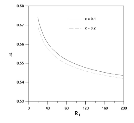
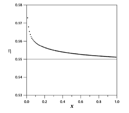
Figure 1: Exponent $\eta$ given by Eq.(15) plotted as a function of $R_{t}$, for $x$=0.1 (solid line) and 0.2 (dashed line) (a), and as a function of $x,$ for $R_{t}$=44 nm (b).

The behavior of $\eta$ in Eq.(15) is presented in Fig.(1). Fig. (1a) shows $\eta$ as a function of $R_{t}$, for 20 nm $\leq R_{t}\leq$ 100 nm, and $\rho_{c}=0.2$ nm. We notice that in this range of $R_{t}$, $0.54<\eta<0.58$. It is also interesting to look at the behavior of $\eta$ as a function of $x$. Fig. (1b) shows $\eta$ as a function of $x$, for $0.01\leq x\leq 1$, $R_{t}=44$ nm, and $\rho_{c}=$ $0.2$ nm. From the curves in Figs. (1a) and (1b), we find that for $x\geqslant 0.05$, $\eta$ turns out to be close to 0.55, as numerically obtained by d’Albuquerque e Castro et al.prl

It is worth commenting on the effect of using a single value of $\eta$, say 0.55, to scale phase diagrams for the core model considered just above. As already pointed out, the diagram for the full strength of the exchange interaction can be obtained from the one corresponding to a reduced interaction $J^{\prime}=xJ$ (with $x<1$) by multiplying the axes $H^{\prime}$ and $D^{\prime}$ of the latter by $1/x^{\eta}$. Thus, an inaccuracy $\delta\eta$ in the value of $\eta$ results in inaccuracies $\delta H$ and $\delta D$ in the coordinates in the scaled diagram. Indeed, if we write $\eta=\eta_{0}\pm\delta\eta$, with $\delta\eta$/$\eta_{0}\ll 1$, we immediately get

$$\left|\frac{\delta H}{H_{0}}\right|=-\ \left(\eta_{0}\ln x\right)\ \left|\frac{\delta\eta}{\eta_{0}}\right|\ ,$$

where $H_{0}=x^{\eta_{0}}H^{\prime}$. Since $\eta_{0}\approx 0.55$ and $\delta\eta/\eta_{0}\approx 0.01$ (estimated from Fig.(1a)), we find that, even for $x$ as small as 0.05, the relative error $\delta H/H_{0}$ is smaller than 2 %. Thus, we do not expect large discrepancies between the calculated phase diagram and the experimental data resulting from such inaccuracy in $\eta$ since a relative error of 2% should not exceed the experimental error.

We remark that the above results for $\eta$ hold also when the core radius corresponds to several interatomic distances and is kept fixed as the exchange interaction is scaled up or down.

We next consider the case in which $\rho_{c}$ is adjusted so as to minimize the energy of the vortex configuration (second core model). From  Eqs.(9) and (10) we obtain the following equation for $\rho_{c}$

$$3\alpha_{n}\frac{\rho_{c}^{3}}{H^{3}}-\beta_{n}\frac{\rho_{c}^{4}}{H^{4}}F(n,\rho_{c}/H)\\ +\frac{\beta_{n}}{2(n+2)}\frac{\rho_{c}^{6}}{H^{6}}G(n,\rho_{c}/H)=\frac{2A}{\mu_{0}M_{0}^{2}H^{2}},$$

where

$$G(n,\rho_{c}/H)=\\ \,{}_{3}F_{2}\left[\left\{\frac{3}{2},2,\frac{5}{2}+n\right\},\left\{3+n,4+2n\right\},-\frac{4\rho_{c}^{2}}{H^{2}}\right]\ .$$

Eq. (LABEL:rhoc) can be solved numerically for $\rho_{c}$ in terms of $H$, $A$, and $n$. We remark that for the core model under consideration, $\rho_{c}$ does not depend on the radius $R$. This follows from the fact that the outer region of the cylinder does not interact with the core (apart from the exchange interaction across the interface between the two regions). As a consequence, for a given value of $\rho_{c}$, the difference between the total energy of two cylinders of the same height but different radii does not depend on $\rho_{c}\,$, hence it does not contribute to the derivative of $E_{tot}^{(V)}$ with respect to $\rho_{c}$. That is to say, the equation for $\rho_{c}$ which minimizes the total energy of the vortex configuration is independent of $R$.

Figure (2) illustrates $M_{z}(\rho)$ for $\ A=87.39$ meV/nm, $M_{0}=1.4\times 10^{6}$ A/m, and two values of $H$, namely 20 and 100 nm. For each $H$, results are presented for $n=$ 2 (dotted line), 4 (dashed line), and 10 (solid line). The values of $A$ and $M_{0}$ correspond to those for Co, and have been taken from Ref.[14]. The value of $\rho_{c}$ in each case has been obtained from Eq.(LABEL:rhoc).

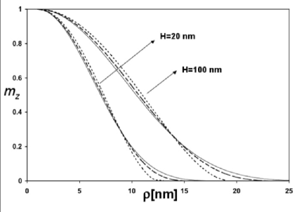
Figure 2: Reduced magnetization $m_{z}=M_{z}/M_{0}$ as a function of $\rho$, for $n=2$ (dotted line), 4 (dashed line), and 10 (solid line). The two sets of curves correspond to $H=$ 20 nm, and 100 nm. Values of $A$ and $M_{0}$ have been taken from Ref. [14], and correspond to those for Co.

In order to investigate the behavior of  magnetic phase diagram upon scaling of the exchange interaction for this second core model, we take $n=$ 4, which according to Fig. (2) provides a physically sound description of the core profile, and calculate the phase diagrams for distinct values of $x$. Fig. (3) shows results for cylinders of Co ($A=87.39$ meV/nm and $M_{0}=1.4\times 10^{6}$ A/m) corresponding to $x=0.12$ (dashed lines) and $x=24$ (dotted lines).

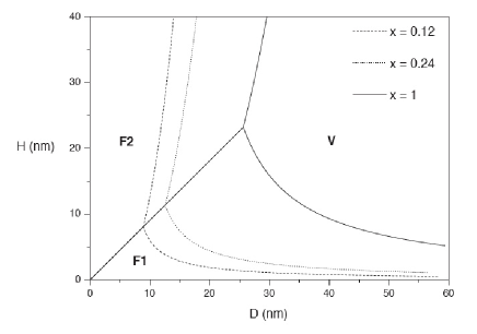
Figure 3: Phase diagram for Co cylinders corresponding to $x=0.12$ (dashed lines), $x=0.24$ (dotted lines) and $x=1$ (solid lines) obtained for core model 2 (see text).

We then find that, for the present core model, the coordinates $(D_{t},H_{t})$ of the triple point follow the relations

$$D_{t}(x) = 25.61\ x^{0.5}$$ (16)

$$H_{t}(x) = 23.22\ x^{0.5}$$ (17)

in which $\eta=0.5$. The diagram for the the full strength of the exchange interaction, $x=1$, is represented by solid line.

We remark that these results holds for any other integer values of $n$, the reason being the fact that since $\rho_{c}$ is adjusted so as to minimize the energy in the vortex configuration, the effective radius of the core turns out to be independent of $n$, as clearly shown in Fig.(2).

V Conclusions

We have carried out a detailed analysis of scaling technique recently proposed by d’Albuquerque e Castro et alprl to investigate the magnetic phase diagram of nanoparticles. As already pointed out, this technique enables us to obtain the phase diagram for particles in the nanometer size range from those corresponding to much smaller particles, in which the exchange interaction has been reduced. The scaling technique is easily implemented and represents a rather useful tool for dealing with nanoparticle systems. In addition, the existence of scaling relations and their connection with the model adopted to describe the magnetic particles bring about interesting theoretical considerations.

The present work sheds light on a very interesting feature of the scaling relations, namely the dependence of the exponent $\eta$ on the model adopted for describing the core of the vortex configuration. Based on a continuous magnetization model, we were able to derive analytical expressions for the total energy in each configuration, which allowed us to determine the exponent $\eta$. We found that in the case of nanoparticles for which the core dimensions, and consequently its contribution to the total energy, can be either neglected or do not change much upon scaling of $A$, $\eta$ turns out to be weakly dependent on $x$ and quite close to 0.55. Nevertheless, when the contribution from the core is relevant and its size upon scaling of $A$ changes so as to minimize the total energy in the vortex configuration, then $\eta$ becomes exactly equal to 0.5.

References

- (1) J. d’Albuquerque e Castro, D. Altbir and J.C. Retamal, P. Vargas, Phys. Rev. Lett. 88, 237202 (2002).
- (2) S. Y. Chou, Proc. IEEE 85, 652 (1997); G. Prinz, Science 282, 1660 (1998).
- (3) J. N. Chapman, P. R. Aitchisom, K. J. Kirk, S. McVitie, J. C. S. Kools, and M. F. Gillies, J. Appl. Phys. 83, 5321 (1998).
- (4) C. A. Ross, M.Hwang, M. Shima, J. Y. Cheng, M. Farhoud, T. A. Savas, Henry I. Smith, W. Schwarzacher, F. M. Ross, M. Redjdal, and F. B. Humphrey, Phys. Rev. B 65, 144417 (2002).
- (5) R. P. Cowburn, D. K. Koltsov, A. O. Adeyeye, and M. E. Welland, D. M. Tricker, Phys. Rev. Lett. 83, 1042 (1999).
- (6) A. Lebib, S. P. Li, M. Natali, and Y.Chen, J. Appl. Phys. 89, 3892 (2001)
- (7) J. Escrig, P. Landeros, J. C. Retamal, D. Altbir, and J. d ’Albuquerque e Castro, Appl. Phys. Lett. 82, 3478 (2003).
- (8) M. Grimsditch, Y. Jaccard and Ivan K.Schuller, Phys. Rev. B 58, 11539 (1998).
- (9) K. Yu Guslienko, Sug-Bong Choe, and Sung-Chul Shin, Appl. Phys. Lett. 76, 3609 (2000)
- (10) C. A. Ross, Henry I. Smith, T. Savas, M. Schattenburg, M. Farhoud, M. Hwang, M, Walsh, M. C. Abraham, R. J. Ram, J. Vac. Sci. Technol. B 17, 3168 (1999).
- (11) A. Aharoni, Introduction to the Theory of Ferromagnetism (Clarendon Press, Oxford, 1996).
- (12) S. Tandom, M. Beleggia, Y. Zhu, M. De Graef, J. Magn. Magn. Mater. 271, 9 (2004).
- (13) see eg. A. Hubert and R. Schäfer, Magnetic Domains: The Analysis of Magnetic Microstructures, Ed. Spinger, Berlin-Heidelberg-New York (1998) and references therein
- (14) see, for ex., N. A. Usov, S.E. Peschany, J. Magn. Magn. Mater. 118, L290 (1993).
- (15) http://magnet.atp.tuwien.ac.at/scholz/projects/diss/html/node86.html