Anderson model out of equilibrium: conductance and Kondo temperature

Abstract

We calculate conductance through a quantum dot weakly coupled to metallic contacts by means of Keldysh out of equilibrium formalism. We model the quantum dot with the SU(2) Anderson model and consider the limit of infinite Coulomb repulsion. We solve the interacting system with the numerical diagrammatic Non-Crossing Approximation (NCA). We calculate the conductance as a function of temperature and gate voltage, from differential conductance (dI/dV) curves. We discuss these results in comparison with those from the linear response approach which can be performed directly in equilibrium conditions. Comparison shows that out of equilibrium results are in good agreement with the ones from linear response supporting reliability to the method employed. The discussion becomes relevant when dealing with general transport models through interacting regions. We also analyze the evolution of the curve of conductance vs gate voltage with temperature. While at high temperatures the conductance is peaked when the Fermi energy coincides with the energy of the localized level, it presents a plateau for low temperatures as a consequence of Kondo effect. We discuss different ways to determine Kondo’s temperature and compare the values obtained in and out of equilibrium.

1 Introduction

Since the first observation of the Kondo effect in semiconducting quantum dots (QD)[1] the study of transport through nanoscopic devices has inspired a rich variety of experimental and theoretical works. Nowadays, measurements of transport properties in such systems, such as current versus bias voltage and conductance, are the main focus of the experiments due to the interesting and unusual features observed [2, 3].

The behavior of the conductance at different temperatures and for different gate voltages has been studied in very general systems, including those showing strong correlations. While at equilibrium almost exact numerical methods have been developed for the theoretical treatment of this problems (numerical renormalization group (NRG)[4] or exact diagonalization (ED)[5]), the ones for non-equilibrium conditions are still in progress. Among them, the Scattering Bethe Ansatz (SBA)[6] and the Time dependent Density Matrix Renormalization Group (t-DMRG)[7] are promising.

In this work we study the transport properties of an interacting QD using the Non-Crossing Approximation (NCA) in its non-equilibrium[8] and equilibrium[9] versions. We consider mandatory the comparison beetwen both schemes to support reliability to the more general procedure dealing with an out of equilibrium calculation. We discuss the results for conductance as function of bias and gate voltage, and moreover, the dependence of transport properties with temperature.

2 Model

We study the transport properties through a quantum dot weak-coupled to metallic contacts and describe the system with the Anderson model,

$$H = \sum_{k\sigma\nu}\epsilon_{k\sigma\nu}c^{{\dagger}}_{k\sigma\nu}c_{k\sigma\nu}+\sum_{\sigma}E_{d}d^{{\dagger}}_{\sigma}d_{\sigma}+Ud^{{\dagger}}_{\uparrow}d_{\uparrow}d^{{\dagger}}_{\downarrow}d_{\downarrow}$$ (1)

$$+ \sum_{k\nu\sigma}V_{k\nu\sigma}c^{{\dagger}}_{k\nu\sigma}d_{\sigma}+H.c.,$$

where $c_{k\sigma\nu}$($c^{\dagger}_{k\sigma\nu}$) is the destruction (creation) operator of an electron with momentum $k$, spin $\sigma$ and lead $\nu=L$ (left) or $R$ (right), and $d_{\sigma}$ ($d^{\dagger}_{\sigma}$) destroys (creates) an electron in the quantum dot.

The non-interacting conduction electrons in the leads are treated as being in thermal and chemical equilibrium with their reservoirs, thus $\epsilon_{k\sigma\nu}=\epsilon_{k\sigma}-\mu_{\nu}$, allowing for different chemical potentials $\mu_{\nu}$ in each of them. For the central region, we consider a spin degenerate localized level with energy $E_{d}$ and Coulomb repulsion $U$. The leads and the dot are connected by means of hybridizations $V_{k\sigma\nu}$.

The physical quantity accessible in transport measurements is the current. As shown by Meir and Wingreen[10], the current through a system described by the Hamiltonian Eq.(1) is given by

$$I = \frac{2\pi e}{h}Tr\int d\omega(\Gamma^{L}f_{L}(\omega)-\Gamma^{R}f_{R}(\omega))\rho_{d}(\omega)$$ (2)

$$+ \frac{2\pi e}{h}Tr\int d\omega(\Gamma^{L}-\Gamma^{R})iG_{d}^{<}(\omega)/2\pi,$$

where $\Gamma^{\nu}_{\sigma}=2\pi\sum_{k}|V_{k\sigma\nu}|^{2}\delta(\omega-\epsilon_{k\sigma\nu})$ is the hybridization function and $f_{L}$($f_{R}$) is the Fermi function for the conduction electrons of the left(right) lead. The functions $\rho_{d}(\omega)$ and $G_{d}^{<}(\omega)$ represent the spectral density and the lesser Green function of the central region respectively. The calculation of such Green functions must be done in presence of the leads and is a non-equilibrium problem which might be handled within Keldysh formalism.

From the results of different applied bias voltages, differential conductance $dI/dV$ curves can be obtained by differentiation of Eq. (2). The value at zero bias $dI/dV|_{0}=G(T)$ represent (the usual equilibrium conductance) at a given temperature. A simplified analytical expression for $G(T)$ can be obtained under the condition of proportional couplings, $\Gamma^{L}_{\sigma}=\alpha\Gamma^{R}_{\sigma}$ [8]

$$G(T)=4\pi\frac{e^{2}}{h}\int d\omega\left(-\frac{\partial f}{\partial\omega}\right)\Gamma(\omega)\rho_{d}(\omega),$$ (3)

where $\Gamma_{\sigma}=\Gamma^{L}_{\sigma}\Gamma^{R}_{\sigma}/(\Gamma^{L}_{\sigma}+\Gamma^{R}_{\sigma})$ is the effective hybridization and $\rho_{d}(\omega)$ is calculated in equilibrium. Thus, in contrast to Eq. (2) ony equilibrium quantities enter Eq. (3).

3 Results

For the treatment of the model in and out of equilibrium, we use the diagrammatic NCA technique[8, 11, 12]. We consider the case of infinite repulsion, $U\rightarrow\infty$. It must be noted that different sets of self-consistent equations have to be solved in order to compute the equilibrium and non-equilibrium Green’s functions. Therefore, computing the current from Eqs (2) and (3) allows us to test the validity of the methods used.

For numerical evaluations, we consider a flat conduction band with band width $2D$ and also take $V_{L}=V_{R}=V$, $\Gamma^{\nu}_{\sigma}=\pi V^{2}/D$. As it is clear from Eq. (2) and Eq. (3), the main dependence on the conductance at low enough temperatures $T$ is given by the spectral weight close to the Fermi level. It is then useful to understand the behavior of the spectral density of the QD for different conditions, specially in the Kondo regime, where an enhanced conductance is expected. In Fig.1 we show the resulting $\rho_{\sigma}$ for different applied bias voltages. We take $\Gamma_{L}=1$ as our unit and set $E_{d}=-4$, $D=10$ and $T=5\times 10^{-5}$. We fix the Fermi level $\epsilon_{F}=0$. Note that $\epsilon_{F}-E_{d}\gg\Gamma_{L}$ so the localized level is always occupied ($\langle n_{\sigma}\rangle\sim 1$). This corresponds to the Kondo regime, in which there is a localized spin interacting with the conduction electrons.

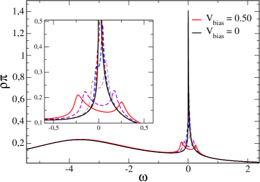
Figure 1: QD spectral density for different applied bias voltages.

At zero bias there are two peaks in the spectral density. The one centered close to $E_{d}$, the charge transfer peak, is the result of a non-interacting orbital hybridizing with a conduction band. If temperature were higher than the relevant low-energy scale of the problem, the Kondo temperature $T_{K}$, this would be the only peak in the spectral density. Since $T$ is very low, the low-energy physics is dominated by the Kondo singlet between conduction electrons and the localized one. The localized spin leads electrons close to Fermi level to suffer spin-flip processes giving rise to a screening effect. This is the reason for the increase of the spectral weight at $\epsilon_{F}$ shown in the figure, which corresponds to the Kondo peak. Its width is related with $T_{K}$. When bias is turned on (dashed curves in Fig. 1) the Fermi level of each metallic contact is shifted. We set $\mu_{L}=-\mu_{R}=eV/2$. This energy shift produces a splitting of the Kondo resonance since conduction electrons coming from both leads contribute to the screening process. As a direct consequence the spectral weight at the equilibrium Fermi level decreases and a lower conductance is expected. In Fig. 2, we show the differential conductance for several temperatures. Since bias voltage is applied symmetrically the current $I(V)$ is an odd function and thus conductance $dI/dV(V)$ an even one. $dI/dV$ curves are Lorentzian-like with the maximum at zero bias. The value at the maximum and the width depend on temperature.

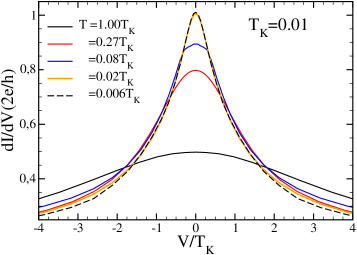
Figure 2: $dI/dV$ vs. $V$ for different temperatures.

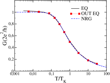
Figure 3: Conductance as a function of temperature obtained from lineal response formalism (continuous curve) and differential conductance curves evaluated at zero bias(dots) and NRG predictions.

From the maximum of the curves of Fig. 2, we can build a point-by-point curve of $G$ vs. temperature. The result is shown in Fig. 3. We show also a continuous line curve which corresponds to an equilibrium calculation of the conductance in the linear-response regime by means of Eq. 3. The dashed line curve is the empirical formula derived from the NRG calculations[13]. For high temperatures $T\gg T_{K}$, there is no Kondo resonance and thus the spectral weight at the Fermi level is low. There is an intermediate region where thermal fluctuations compete, and at low enough temperatures $T\ll T_{K}$, the Kondo effect is fully developed and conductance tends to a saturation value. However, at $T\ll T_{K}$, the NCA overestimates the Friedel’s sum rule and therefore the conductance exceeds the unitary limit.

As it is shown in Fig. 3, there is an excellent agreement between the results from the non-equilibrium calculation and the equilibrium ones. Moreover, there is also a great correspondence to the results from NRG. We stress that the calculation of linear response conductance implies only equilibrium quantities while the out of equilibrium solving procedure is more complex and deals with lesser and greater Green functions. Since the first of this approaches is valid just under the condition of proportional couplings, the agreement we find is a useful check that supports reliability to the most general procedure based on the calculation of the current by means of Eq. (2).

Figure 4: Conductance as a function of gate voltage $V_{g}$ for different temperatures obtained from lineal response formalism (continuous curve) and from differential conductance curves evaluated at zero bias(red dots).

We turn now the discussion to the conductance as a function of gate voltage $V_{g}$. The energy of the localized level of the QD is proportional to this voltage $eV_{g}=-E_{d}$ and thus it is possible to perform a transistor-type experiment by the control of this parameter. In Fig. 4, we present the NCA results for different temperatures. The understanding of this outcome is directly connected to our previous analysis of the spectral density. For high temperatures (black continuous line in the figure) conductance shows just a symmetric peak centered at $V_{g}=0$. This corresponds to the localized level placed at the Fermi energy, the optimum condition for conduction electrons to pass from left to right metallic contact. For temperatures lower than $T_{K}$ (dashed curves in the figure) the behavior is completely different. As soon as the energy of the localized level is below the Fermi energy, the Kondo effect develops and the spectral density shows not only the charge transfer peak but also the Kondo resonance. This is the reason for the plateau of conductance as a function of gate voltage. Our results qualitative agree with those obtained previously with NRG [14]. We bring more details on the evolution with temperature. As it is shown in Fig.4, at finite temperature conductance start to decay at some $V_{g}$. This feature has to do with the fact that $T_{K}\sim\exp\{E_{d}\}$, i.e. smaller for more negative values of $E_{d}$. Since temperature is finite, $T$ turns bigger than $T_{K}(E_{d})$ at some point destroying the Kondo effect and the plateau. It must be noticed that for $T<T_{K}$, the NCA results are not reliable within the empty orbital regime, $E_{d}\geq 0$, due to the appearance of a spike with non physical spectral weight at the Fermi energy.

For $T=1.5\times 10^{-4}$ we show (with dots) in Fig. 4 the values of conductance obtained by the procedure stated previously from the calculations out of equilibrium. In the inset of the figure we show differential conductance curves for several $V_{g}$. We observe that the maximum of the conductance keeps the same while the curves get narrower for greater values of gate voltage. This is a direct indication of the variation of $T_{K}$ with $V_{g}$.

There are three different way to define the characteristic energy scale $T_{K}$ from the physical magnitudes addressed in this work: At equilibrium it can be obtained from the half-width at half of the maximum (HWHM) of spectral density for $T\rightarrow 0$ ($T_{K}^{\rho}$). Out of equilibrium, from the HWHM of differential conductance curves, $T_{K}^{dI/dV}$. From the equilibrium conductance, $T_{K}^{G}$ is defined as the temperature such that $G(T)=G(0)/2$. From our results, $T_{K}^{G}=8.2\ 10^{-3}$, $T_{K}^{\rho}=9.1\ 10^{-3}=1.11T_{K}^{G}$ and $T_{K}^{dI/dV}=12.1\ 10^{-3}=1.48T_{K}^{G}$. As expected, the three values are of the same order of magnitude. These realtions can be used to estimate any one of them in a case it might not be accessible and to test the model.

4 Conclusions

In this work we study the transport through an interacting quantum dot described with the Anderson model. We use the NCA to calculate the conductance as a function of bias and gate voltage, and temperature. We find a great agreement between the results from the non-equilibrium calculations and those from the linear response regime which imply only equilibrium quantities. The results for conductance versus temperature also agrees with those from NRG calculations. We analyze the conductance as a function of gate voltage and observe the formation of a plateau for low enough temperatures within the Kondo regime in agreement with previous results. As a consequence of finite temperature, the conductance decays for a given value of the gate voltage destroying the plateau. We finally discuss several methods, in and out of equilibrium, which allows the determination of Kondo temperature. We find that the values obtained are of the same order and provide numerical relations beetwen them. While the conductance at equilibrium of the model is known from NRG calculations, we show that the NCA is able to provide reliable results at a lower computational cost, and to extend the results out of equilibrium, for which few alternative techniques exist. Moreover, the NRG can miss structures in the spectral density which are not near to the Fermi energy [15, 16]. This turned out to be important to explain a plateau observed in $G(T)$ in $C_{60}$ QDs [2] on the triplet side of a quantum phase transition, using the NCA [16].

5 Acknowledgments

Two of us (A. A. A. and A. M. L.) are partially supported by CONICET, Argentina. This work was partially supported by PIP No 11220080101821 of CONICET, and PICT Nos 2006/483 and R1776 of the ANPCyT.

References

- [1] D. Goldhaber-Gordon et al., Nature 391, 156 (1998).
- [2] N. Roch et al., Nature 453, 633 (2008).
- [3] J. J. Parks et al., Science 328, 1370 (2010).
- [4] R. Bulla et al., Rev. Mod. Phys. 80, 395 (2008).
- [5] M. Caffarel et al., Phys. Rev. Lett. 72, 1545 (1994).
- [6] P. Metha and N. Andrei, Phys. Rev. Lett. 96, 216802 (2006).
- [7] A. J. Daley et al., J. Stat. Mech. (2004) P04005.
- [8] N. S. Wingreen and Y. Meir, Phys. Rev. B 49, 11040 (1994).
- [9] N. E. Bickers et al., Rev. Mod. Phys. 59 845 (1987).
- [10] Y. Meir and N. S. Wingreen, Phys. Rev. Lett. 68, 2512 (1992).
- [11] M. Hettler, J. Kroha and S. Herschfield, Phys. Rev. B 58, 5649 (1998).
- [12] P. Roura-Bas, Phys. Rev. B 81, 155327 (2010).
- [13] T. A. Costi, Phys. Rev. Lett. 85, 1504 (2000).
- [14] W. Izumida, O. Sakai, and S. Suzuki, J. Phys. Soc. Jpn. 70, 1045 (2001͒).
- [15] L. Vaugier, A.A. Aligia and A.M. Lobos, Phys. Rev. B 76, 165112 (2007); Phys. Rev. Lett. 99, 209701 (2007)
- [16] P. Roura Bas and A. A. Aligia, Phys. Rev. B 80, 035308 (2009); J. Phys. Cond. Matt. 22, 025602 (2010).