On the Transport Diamonds and Zero Current Anomaly in InGaAs/InP and GaAs/AlGaAs

Abstract

In the quantum Hall effect (QHE) the differential resistivity $r_{xx}\equiv r$ vanishes within a range where the Hall resistivity forms a plateau. A microscopic theory is developed, starting with a crystal lattice, setting up a BCS-like Hamiltonian in terms of composite bosons, and using statistical mechanical method. The main advantage of our bosonic theory is its capability of explaning the plateau formation in the Hall resistivity, which is assumed in the composite fermion theories. In the QHE under radiation, the resistivity vanishes within a range with no plateau formation. This is shown in terms of two-channels model, one channel excited by radiation where the supercurrents run and the other (base) channel in which the normal currents run. The transport diamonds (TD) and the zero direct current anomaly (ZCA) occur when the resistivity $r$ is measured as a function of magnetic field and direct current (DC). The spiral motion of an electron under a magnetic field can be decomposed into two, the cyclotron motion with the cyclotron mass $m^{*}$ and the guiding center motion with the magnetotransport $M^{*}$. The quantization of the motion generates magnetic oscillations in the density of states. The magnetoconductivity is calculated, using kinetic theory and quantum statistical mechanics. The TR and ZCA are shown to be a breakdown of QHE. The integer QHE minima are shown to become the Shubnikov-de Haas (SdH) maxima progressively as the DC increases. The ZCA at low temperatures ($T=0.253$–$1.2$ K) is temperature-dependent, which is caused by the electron-optical-phonon scattering.

I INTRODUCTION

Recently, Studenikin et al. Studenikin discovered transport diamonds (TR) and zero-current anomaly (ZCA) in In_xGa_1-xAs/InP and GaAs/AlGaAs. The TR and ZCA occur when the differential resistance $r_{xx}=dV_{xx}/dI$ of a Hall bar sample after the red-light illumination is plotted in the plane of the magnetic field and the direct current (DC). See Fig. 4, which is reproduced from Ref. Studenikin , Fig. 2. Diamond-shaped regions developing from SdH minima are called transport diamonds and a sharp dip in $r_{xx}$ appearing at a narrow horizontal line at zero DC is called a zero-current anomaly. The details of the experiments and theoretical backgrounds can be found in Ref. Studenikin . The original authors Studenikin suggested an interpretation: the breakdown of the quantum Hall effect (QHE). We shall show in the present work that this is indeed the case based on the composite (c-)boson model, the model originally introduced by Zhang, Hansson and Kivelson Zhang and later developed by Fujita’s group Fujita_1 . In the prevalent theories Ezawa , the QHE is discussed in terms of the c-fermions. Jain The formation of the Hall resistivity plateau where the resistivity vanishes, is assumed, however. In our c-boson theory, the plateau formation is explained from the first principles. In Sec. II, we review our microscopic theory of the QHE. The QHE for a system subjected to a radiation is developed and discussed in Sec. III. The density of Landau states and statisical weight in two dimensions (2D) are calculated in Sec. IV. Shubnikov-de Haas (SdH) oscillations Shubnikov in the magnetoconductivity and de Haas-van Alphen (dHvA) oscillations Haas in the magnetic susceptibility, are jointly called magnetic oscillations. They originate in the oscillations in statistical weight. Magnetic oscillations are often discussed, using a so-called Dingle temperature Dingle . But this is a phenomenological treatment, which must be avoided. Following our previous work Fujita_6 , we present a microscopic theory of the SdH oscillations for a 2D system in Sec. V. The TR and ZCA are discussed in Sec. VI.

II INTEGER QUANTUM HALL EFFECT

If a magnetic field $\mathbf{B}$ is applied slowly, then the classical electron can continuously change from the straight line motion at zero field to the curved motion at a finite $B$ (magnitude). Quantum mechanically, the change from the momentum state to the Landau state requires a perturbation. We choose for this perturbation the phonon exchange attraction between the electron and the fluxon (elementary magnetic flux). Consider an electron with a few fluxons. If the magnetic field is applied slowly, the energy of the electron does not change but the cyclotron motion always acts so as to reduce the magnetic fields surrounding the electron. Hence the total energy of the composite of an electron and fluxon is less than the electron energy plus the unperturbed field energy. In other words, the composite (c-)particle is stable against the break-up, and it is in a bound (negative energy) state. The c-particle is simply a dressed electron carrying $Q$ fluxons. $Q=1,2,\dots$. Originally, the c-particle was introduced as a composite of one electron attached with a number of Chern-Simons gauge objects. Ezawa These objects are neither bosons nor fermions, and hence the statistics of the composite is not clear. The basic particle property (countability) of the fluxons is known as the flux quantization, see Eq. (II.15). We assume that the fluxon is an elementary fermion with zero mass and zero charge, which is supported by the fact that the fluxon, the quantum of the magnetic field $\mathbf{B}$, cannot disappear at a sink unlike the bosonic photon, the quantum of the electric field $\mathbf{E}$ Fujita_1 . Fujita and Morabito Fujita_2 showed that the center-of-mass (CM) of a composite moves following the Ehrenfest-Oppenheimer-Bethe’s (EOB) rule Ehrenfest : the composite is fermionic (bosonic) if it contains an odd (even) number of elementary fermions. Hence the quantum statistics of the c-particle is established.

At the Landau level (LL) occupation number, also called the filling factor, $\nu=1/Q$, $Q$ odd, the c-bosons with $Q$ fluxons are generated and can condense below certain critical temperature $T_{c}$. The Hall resistivity plateau is caused by kind of the Meissner effect as explained later.

We develop a theory for GaAs/AlGaAs heterojunction, the theory which can also be applied to InGaAs/InP quantum well. GaAs forms a zincblende lattice. We assume that the interface is in the plane $(001)$. The Ga³⁺ ions form a square lattice with the sides directed in $[110]$ and $[1\bar{1}0]$. The “electron” (wave packet) with a negative charge $-e$ will then move isotropically with an effective mass $m_{1}$. The As^3- ions also form a square lattice at a different height in $[001]$. The “holes”, each having a positive charge (+e), will move similarly with an effective mass $m_{2}$. A longitudinal phonon moving in $[110]$ or in $[1\bar{1}0]$ can generate a charge (current) density variation, establishing an interaction between the phonon and the electron (fluxon). If one phonon exchange is considered between the electron and the fluxon, a second-order perturbation calculation establishes an effective electron-fluxon interaction

$$\left|V_{q}V_{q}^{\prime}\right|\frac{\hbar\omega_{q}}{\left(\varepsilon_{|\mathbf{p}\boldsymbol{+}\mathbf{q}|}-\varepsilon_{p}\right)^{2}-(\hbar\omega_{q})^{2}},$$ (II.1)

where $\mathbf{q}$ ($\hbar\omega_{q}$) is the phonon momentum (energy), $V_{q}(V_{q}^{\prime})$ the interaction strength between the electron (fluxon) and the phonon. If the energies $\left(\varepsilon_{|\mathbf{p}\boldsymbol{+}\mathbf{q}|},\varepsilon_{p}\right)$ of the final and initial electron states are equal, the effective interaction is negative (attractive) as seen from Eq. (II.1).

Following Bardeen-Cooper-Schrieffer (BCS) Bardeen , we start with a Hamiltonian $H$ with the phonon variables eliminated:

$$H= \sum_{k}\sum_{s}\varepsilon_{k}^{(1)}n_{\text{k}s}^{(1)}+\sum_{k}\sum_{s}\varepsilon_{k}^{(2)}n_{\text{k}s}^{(2)}+\sum_{k}\sum_{s}\varepsilon_{k}^{(3)}n_{\text{k}s}^{(3)}$$

$$\mbox{}-v_{0}\sideset{}{{}^{\prime}}{\sum}_{\mathbf{q}}\sideset{}{{}^{\prime}}{\sum}_{\mathbf{k}}\sideset{}{{}^{\prime}}{\sum}_{\mathbf{k}\boldsymbol{{}^{\prime}}}\sum_{s}\Big{[}B_{\mathbf{k}\boldsymbol{{}^{\prime}}\mathbf{q}s}^{(1)\dagger}B_{\mathbf{kq}s}^{(1)}+B_{\mathbf{k}\boldsymbol{{}^{\prime}}\mathbf{q}s}^{(1)\dagger}B_{\mathbf{kq}s}^{(2)\dagger}$$

$$\mbox{}+B_{\mathbf{k}\boldsymbol{{}^{\prime}}\mathbf{q}s}^{(2)}B_{\mathbf{kq}s}^{(1)}+B_{\mathbf{k}\boldsymbol{{}^{\prime}}\mathbf{q}s}^{(2)}B_{\mathbf{kq}s}^{(2)\dagger}\Big{]},$$ (II.2)

where $n_{\mathbf{k}s}^{(j)}$ is the number operator for the “electron”(1) [“hole”(2), fluxon (3)] at momentum $\mathbf{k}$ and spin $s$ with the energy $\varepsilon_{ks}^{(j)}$. We represent the “electron” (“hole”) number $n_{\mathbf{k}s}^{(j)}$ by $c_{\mathbf{k}s}^{(j)\dagger}c_{\mathbf{k}s}^{(j)}$, where $c(c^{\dagger})$ are annihilation (creation) operators satisfying the Fermi anticommutation rules:

$$\left\{c_{\mathbf{k}s}^{(i)},c_{\mathbf{k}\boldsymbol{{}^{\prime}}s^{\prime}}^{(j)\dagger}\right\} \equiv c_{\mathbf{k}s}^{(i)}c_{\mathbf{k}\boldsymbol{{}^{\prime}}s^{\prime}}^{(j)\dagger}+c_{\mathbf{k}\boldsymbol{{}^{\prime}}s^{\prime}}^{(j)\dagger}c_{\mathbf{k}s}^{(i)}=\delta_{\mathbf{k,k^{\prime}}}\delta_{\mathbf{s,s^{\prime}}}\delta_{i,j},$$

$$\left\{c_{\mathbf{k}s}^{(i)},c_{\mathbf{k}\boldsymbol{{}^{\prime}}s^{\prime}}^{(j)}\right\} =0.$$ (II.3)

We represent the fluxon number $n_{\mathbf{k}s}^{(3)}$ by $a_{\mathbf{k}s}^{\dagger}a_{\mathbf{k}s}$, with $a(a^{\dagger})$, satisfying the anticommutation rules, (II.3).

$$B_{\mathbf{kq}s}^{(1)\dagger} \equiv c_{\mathbf{k}\boldsymbol{+}\mathbf{q}/2\,s}^{(1)\dagger}a_{\boldsymbol{-}\mathbf{k}\boldsymbol{+}\mathbf{q}/2\,-s}^{\dagger},$$

$$B_{\mathbf{kq}s}^{(2)} \equiv c_{\mathbf{k}\boldsymbol{+}\mathbf{q}/2\,s}^{(2)}a_{\boldsymbol{-}\mathbf{k}\boldsymbol{+}\mathbf{q}/2\,-s}.$$ (II.4)

The prime on the summation in Eq. (II.2) means the restriction: $0<\varepsilon_{ks}^{(j)}<\hbar\omega_{\text{D}}$, $\omega_{\text{D}}$ = Debye frequency. If the fluxons are replaced by the conduction electrons (“electrons”, “holes”) our Hamiltonian $H$ is reduced to the original BCS Hamiltonian, Eq. (24) of Ref. Bardeen . The “electron” and “hole” are generated, depending on the energy contour curvature sign Fujita_3 . For example, only “electrons” (“holes”), are generated for a circular Fermi surface with the negative (positive) curvature whose inside (outside) is filled with electrons. Since the phonon has no charge, the phonon exchange cannot change the net charge. The pairing interaction terms in Eq. (II.2) conserve the charge. The term $-v_{0}B_{\mathbf{k}\boldsymbol{{}^{\prime}}\mathbf{q}s}^{(1)\dagger}B_{\mathbf{kq}s}^{(1)}$, where $v_{0}\equiv\left|V_{q}V_{q}^{\prime}\right|(\hbar\omega_{0}A)^{-1}$, $A$ = sample area, is the pairing strength, generates the transition in the “electron” states. Similarly, the exchange of a phonon generates a transition in the “hole” states, represented by $-v_{0}B_{\mathbf{k}\boldsymbol{{}^{\prime}}\mathbf{q}s}^{(2)}B_{\mathbf{kq}s}^{(2)\dagger}$. The phonon exchange can also pair-create and pair-annihilate “electron” (“hole”)-fluxon composites, represented by $-v_{0}B_{\mathbf{k}\boldsymbol{{}^{\prime}}\mathbf{q}s}^{(1)\dagger}B_{\mathbf{kq}s}^{(2)\dagger}$, $-v_{0}B_{\mathbf{k}\boldsymbol{{}^{\prime}}\mathbf{q}s}^{(2)}B_{\mathbf{kq}s}^{(1)}$. At 0 K, the system can have equal numbers of $-(+)$ c-bosons, “electrons” (“hole”) composites, generated by $-v_{0}B_{\mathbf{k}\boldsymbol{{}^{\prime}}\mathbf{q}s}^{(1)\dagger}B_{\mathbf{kq}s}^{(2)\dagger}$.

The c-bosons, each with one fluxon, will be called the fundamental (f) c-bosons. At a finite temperature, there are moving (non-condensed) fc bosons. Their energies $w_{q}^{(j)}$ are obtained from Fujita_4 :

$$w_{q}^{(j)}\Psi(\mathbf{k,q})= \varepsilon_{|\mathbf{k}\boldsymbol{+}\mathbf{q}|}^{(j)}\Psi(\mathbf{k,q})-(2\pi\hbar)^{-2}v_{0}^{*}$$

$$\times\int^{\prime}d^{2}k^{\prime}\Psi(\mathbf{k}\boldsymbol{{}^{\prime}},\mathbf{q}),$$ (II.5)

where $\Psi(\mathbf{k,q})$ is the reduced wavefunction for the fc-boson; we neglected the fluxon energy. The $v_{0}^{*}$ denotes the strength after the ladder diagram binding, see below. For small $q$, we obtain a solution of Eq. (II.5) as

$$w_{q}^{(j)}=\omega_{0}+(2/\pi)v_{\text{F}}^{(j)}q,\quad w_{0}=\frac{-\hbar\omega_{\text{D}}}{\exp(v_{0}^{*}D_{0})^{-1}-1},$$ (II.6)

where $v_{\text{F}}^{(j)}\equiv(2\varepsilon_{\text{F}}/m_{j})^{1/2}$ is the Fermi velocity and $D_{0}\equiv D(\varepsilon_{\text{F}})$ the density of states per spin. The brief derivation of Eqs. (II.5) and (II.6) is given in Appendix A. Note that the energy $w_{q}^{(j)}$ depends linearly on the momentum magnitude $q$.

The system of free fc-bosons undergoes a Bose-Einstein condensation (BEC) in 2D at the critical temperature Fujita_5

$$k_{\text{B}}T_{c}=1.24\,\hbar v_{\text{F}}n_{0}^{1/2}.$$ (II.7)

A brief derivation of Eq. (II.7) is given in Appendix B. The interboson distance $R_{0}\equiv n_{0}^{1/2}$ calculated from this expression is $1.24\hbar v_{\text{F}}(k_{\text{B}}T_{c})^{-1}$. The boson size $r_{0}$ calculated from Eq. (II.6), using the uncertainty relation ($q_{\text{max}}r_{0}\sim\hbar$) and $|w_{0}|\sim k_{\text{B}}T_{c}$ is $(2/\pi)\hbar v_{\text{F}}(k_{\text{B}}T_{c})^{-1}$, which is a few times smaller than $R_{0}$. Hence, the fc-bosons do not overlap in space, and the model of free bosons is justified. For GaAs/AlGaAs, $m^{*}=0.067\,m_{e}$, $m_{e}$ = electron mass. For the 2D electron density $10^{11}$ cm^-2, we have $v_{\text{F}}=1.36\times 10^{6}$ cm s^-1. Not all electrons are bound with fluxons since the simultaneous generations of $\pm$ fc-bosons is required. The minority carrier (“hole”) density controlls the fc-boson density. For $n_{0}=10^{10}$ cm^-2, $T_{c}=1.29$ K, which is reasonable.

In the presence of Bose condensate below $T_{c}$ the unfluxed electron carries the energy Fujita_5

$$E_{k}^{(j)}=\sqrt{\varepsilon_{k}^{(f)2}+\triangle^{2}},$$ (II.8)

where the quasi-electron energy gap $\triangle$ is the solution of

$$1= v_{0}D_{0}\int_{0}^{\hbar\omega_{\text{D}}}d\varepsilon\frac{1}{(\varepsilon^{2}+\triangle^{2})^{1/2}}$$

$$\times\left\{1+\exp\left[-\beta(\varepsilon^{2}+\triangle^{2})^{1/2}\right]\right\}^{-1},\quad\beta\equiv\frac{1}{k_{\text{B}}T}.$$ (II.9)

Note that the gap $\triangle$ depends on the temperature $T$. At the critical temperature $T_{c}$, there is no Bose condensate and hence $\triangle$ vanishes.

Now the moving fc-boson below $T_{c}$ has the energy $\tilde{w}_{q}$ obtained from

$$\tilde{w}_{q}^{(j)}\Psi(\mathbf{k},\mathbf{q})= E_{|\mathbf{k}\boldsymbol{+}\mathbf{q}|}^{(j)}\Psi(\mathbf{k},\mathbf{q})-(2\pi\hbar)^{-2}v_{0}^{*}$$

$$\times\int^{\prime}d^{2}k^{\prime}\Psi(\mathbf{k}\boldsymbol{{}^{\prime}},\mathbf{q}).$$ (II.10)

We obtain after solving Eq. (II.10):

$$\tilde{w}_{q}^{(j)}=\tilde{w}_{0}+(2/\pi)v_{\text{F}}^{(j)}q\equiv w_{0}+\varepsilon_{g}+(2/\pi)v_{\text{F}}^{(j)}q,$$ (II.11)

where $\tilde{w}_{0}(T)$ is determined from

$$1=D_{0}\nu_{0}\int_{0}^{\hbar\omega_{\text{D}}}d\varepsilon\left[\left|\tilde{w_{0}}\right|+(\varepsilon^{2}+\triangle^{2})^{1/2}\right]^{-1}.$$ (II.12)

The energy difference:

$$\tilde{w}_{0}(T)-w_{0}\equiv\varepsilon_{g}(T)$$ (II.13)

represents the $T$-dependent energy gap. The energy $\tilde{w}_{q}$ is negative. Otherwise, the fc-boson should break up. This limits $\varepsilon_{g}(T)$ to be $|w_{0}|$ at 0 K. The fc-boson energy gap $\varepsilon_{g}$ declines to zero as the temperature approaches $T_{c}$ from below.

The fc-boson, having the linear dispersion (II.11) can move in all directions in the plane with the constant speed $(2/\pi)v_{\text{F}}^{(j)}$ as seen from Eq. (II.11). The supercurrent is generated by the $\pm$ fc-bosons condensed monochromatically at the momentum directed along the sample length. The supercurrent density (magnitude) $J$, calculated by the rule: (charge $e^{*}$) $\times$ (carrier density $n_{0}$) $\times$ (drift velocity $v_{d}$), is

$$J\equiv e^{*}n_{0}v_{d}=e^{*}n_{0}(2/\pi)\left|v_{\text{F}}^{(1)}-v_{\text{F}}^{(2)}\right|.$$ (II.14)

The induced Hall field (magnitude) $E_{\text{H}}$ equals $v_{d}B$. The magnetic flux is quantized

$$BA=n_{\phi}(h/e),\quad n_{\phi}\text{ = fluxon density}.$$ (II.15)

Hence, we obtain

$$\rho_{\text{H}}\equiv\frac{E_{\text{H}}}{J}=\frac{v_{d}B}{en_{0}v_{d}}=\frac{1}{en_{0}}n_{\phi}\left(\frac{h}{e}\right).$$ (II.16)

If $n_{\phi}=n_{0}$ valid at $\nu=1$, we obtain $\rho_{\text{H}}=h/e^{2}$ in agreement with the plateau value observed.

The model can be extended to the integer QHE at $\nu=P$, $P=1,2,\dots$. The field magnitude is less. The LL degeneracy $eB\!A/h$ is linear in $B$, and hence the lowest $P$ LL’s must be considered. The fc-boson density $n_{0}$ per LL is the electron density $n_{e}$ over $P$ and the fluxon density $n_{\phi}$ is the boson density $n_{0}$ over $P$:

$$n_{0}=n_{e}/P,\quad n_{\phi}=n_{0}/P.$$ (II.17)

At $\nu=1/2$ there are c-fermions, each with two fluxons. The c-fermions have a Fermi energy. The $\pm$ c-fermions have effective masses. The Hall resistivity $\rho_{\text{H}}$ has a $B$-linear behavior while the resistivity $\rho$ is finite. In our theory the integer $P$ is the number of the LL’s occupied by the c-fermions.

Our Hamiltonian in Eq. (II.2) can generate and stabilize the c-particles with an arbitrary number of fluxons. For example, a c-fermion with two fluxons is generated by two sets of the ladder diagram bindings, each between the electron and the fluxon. The ladder diagram binding arises as follows. Consider a hydrogen atom. The Hamiltonian contains kinetic energies of the electron and the proton and the attractive Coulomb interaction. If we regard the Coulomb interaction as a perturbation and use a perturbation theory, we can represent the interaction process by an infinite set of ladder diagrams, each ladder step connecting the electron line and the proton line. The energy eigenvalues of this system is not obtained by using the perturbation theory but they are obtained by solving the Schrödinger equation directly. This example indicates that a two-body bound state is represented by an infinite set of ladder diagrams and that the binding energy (the negative of the ground-state energy) is calculated by a non-perturbative method.

Jain introduced the effective magnetic field Jain

$$B^{*}\equiv B-B_{\nu}=B-(1/\nu)n_{e}(h/e)$$ (II.18)

relative to the standard field for the composite (c-)fermion. We extend this idea to the bosonic (odd-denominator) fraction. This means that the c-particle moves field-free at the exact fraction. The movement of the guiding centers (the CM of the c-particle) can occur as if they are subjected to no magnetic field at the exact fraction. The excess (or deficit) of the magnetic field is simply the effective magnetic field $B^{*}$. The plateau in $\rho_{\text{H}}$ is formed due to kind of the Meissner effect. Consider the case of zero temperature near $\nu=1$. Only the system energy $E$ matters. The fc-bosons are condensed with the ground-state energy $w_{0}$, and hence the system energy $E$ at $\nu=1$ is $2N_{0}w_{0}$, where $N_{0}$ is the number of $-$ fc-bosons (or $+$ fc-bosons). The factor 2 arises since there are $\pm$ fc-bosons. Away from $\nu=1$, we must add the magnetic field energy $(2\mu_{0})^{-1}A(B^{*})^{2}$, so that

$$E=2N_{0}w_{0}+(2\mu_{0})^{-1}A(B^{*})^{2}.$$ (II.19)

When the field is reduced, the system tries to keep the same number $N_{0}$ by sucking in the flux lines. Thus the magnetic field becomes inhomogeneous outside the sample, generating the extra magnetic field energy $(2\mu_{0})^{-1}A(B^{*})^{2}$. If the field is raised, the system tries to keep the same number $N_{0}$ by expeling out the flux lines. The inhomogeneous fields outside raise the field energy by $(2\mu_{0})^{-1}A(B^{*})^{2}$. There is a critical field $B_{c}^{*}=(4\mu_{0}|w_{0}|)^{1/2}$. Beyond this value, the superconducting state is destroyed, which generates a symmetric exponential rise in the resistance $R$. In our discussion of the Hall resistivity plateau we used the fact that the ground-state energy $w_{0}$ of the fc-boson is negative, that is, the c-boson is bound. Only then the critical field $B_{c}^{*}=(4\mu|w_{0}|)^{1/2}$ can be defined. Here the phonon exchange attraction played an important role. The repulsive Coulomb interaction, which is the departure point of the prevalent fermionic theories Ezawa ; Jain , cannot generate a bound state.

In the presence of the supercondensate, the non-condensed c-boson has an energy gap $\varepsilon_{g}$. Hence, the non-condensed c-boson density has the activation energy type exponential temperature-dependence:

$$\exp[-\varepsilon_{g}/(k_{\text{B}}T)].$$ (II.20)

Some authors argue that the energy gap $\varepsilon_{g}$ for the integer QHE is due to the LL separation = $\hbar\omega_{0}$. But the separation $\hbar\omega_{c}$ is much greater than the observed $\varepsilon_{g}$. Besides, from this view one cannot obtain the activation-type energy dependence.

The BEC occurs at each LL, and therefore the c-boson density $n_{0}$ is smaller for high $P$, see Eq. (II.17), and the strengths become weaker as $P$ increases. The most significant advantage of our bosonic theory is that we are able to explain why the plateaus in the Hall resistivity is developed when the resistivity is zero as the magnetic field is varied. This plateau formation is phenomenologically assumed in the fermionic theories. Ezawa ; Jain

III QUANTUM HALL EFFECT UNDER RADIATION

The experiments by Mani et al. Mani_1 and Zodov et al. Zudov indicate that the applied radiation excites a large number of “holes” in the system. Using these “holes” and the preexisting “electrons” the phonon exchange can pair-create $\pm$ c-bosons, that condense below $T_{c}$ in the excited (upper) channel. The c-bosons condensed with the momentum along the sample length are responsible for the supercurrent. In the presence of the condensed c-bosons, the non-condensed c-bosons have an energy gap $\varepsilon_{g}$, and therefore they are absent below $T_{c}$. The fermionic currents in the base channel cannot be suppressed by the supercurrents since the energy levels are different between the excited and base channels. These c-fermions contribute a small normal current. They are subject to the Lorentz force: $\mathbf{F}=q(\mathbf{E}\boldsymbol{+}\mathbf{v}\boldsymbol{\times}\mathbf{B})$, and hence they generate a Hall field $E_{\text{H}}$ proportional to the field $B$. This is the main feature difference from the usual QHE (under no radiation).

In the neighborhood of the QHE at $\nu=1$, the current carriers in the base and excited channels are, respectively, c-fermions and condensed c-bosons. The currents are additive. We write down the total current density $j$ as the sum of the fermionic current density $j_{f}$ and the bosonic current density $j_{b}$:

$$j=j_{f}+j_{b}=en_{f}v_{f}+en_{b}v_{b},$$ (III.1)

where $v_{f}$ and $v_{b}$ are the drift velocities of the c-fermions and c-bosons. The Hall fields $E_{\text{H}}$ are additive, too. Hence we have

$$E_{\text{H}}=E_{\text{H},f}+E_{\text{H},b}=v_{f}B+v_{b}B.$$ (III.2)

The Hall effect condition ($E_{\text{H}}=v_{d}B$) applies separately for the c-fermions and c-bosons. We therefore obtain

$$R_{\text{H}}=\frac{E_{\text{H}}}{j}=\frac{v_{f}B+v_{b}B}{n_{f}v_{f}+n_{b}v_{b}}\frac{1}{e}.$$ (III.3)

Far away from the midpoint of the zero-resistance stretch, the c-bosons are absent and hence the Hall resistivity $R_{\text{H}}$ becomes $B/(en_{f})$:

$$R_{\text{H}}=B/(en_{f})\quad\text{(far away)},$$ (III.4)

after the cancellation of $v_{f}$. At the midpoint the c-bosons are dominant. Then, the Hall resistivity $R_{\text{H}}$ is approximately equal to $h/e^{2}$ since

$$\frac{E_{\text{H}}}{j}\cong\frac{v_{b}B}{en_{b}v_{b}}\cong\frac{h}{e^{2}}\frac{n_{\phi}}{n_{b}}=\frac{h}{e^{2}}\quad\text{(midpoint)},$$ (III.5)

where we used the flux quantization [$B=(h/e)n_{\phi}$], and the fact that the flux density $n_{\phi}$ equals the c-boson density $n_{b}$ at $\nu=1$. The Hall resistivity $R_{\text{H}}=E_{\text{H}}/j$ is not exactly equal to $h/e^{2}$ since the c-fermion current density $en_{f}v_{f}$ is much smaller than the supercurrent density $en_{b}v_{b}$, but it does not vanish. In the horizontal stretch the system is superconducting, and hence the supercurrent dominates the normal current: $en_{b}v_{b}\gg en_{f}v_{f}$. The deviation $\Delta R_{\text{H}}$ is, using Eq. (III.3),

$$\Delta R_{\text{H}} =\frac{v_{f}B+v_{b}B}{e(n_{f}v_{f}+n_{b}v_{b})}-\frac{v_{f}B}{en_{f}v_{f}}$$

$$\simeq\frac{n_{b}B}{en_{b}v_{b}}\simeq\frac{h}{e^{2}}.$$ (III.6)

If the field $B$ is raised (or lowered) a little from the midpoint, $\Delta R_{\text{H}}$ is a constant ($h/e^{2}$) due to the Meissner effect. If the field is raised high enough, the superconducting state is destroyed and the normal current sets in, generating a finite resistance and a vanishing $\Delta R_{\text{H}}$. Hence the deviation $\Delta R_{\text{H}}$ and the diagonal resistance $R_{xx}$ are closely correlated as observed by Mani Mani_1 .

In Fig. 2 of Ref. Mani_1 (not shown here), we can see that in the range, where the SdH oscillations are observed for the resistance without radiation, the signature of oscillations also appear for the resistance $R_{xx}$ with radiation. The SdH oscillations arise only for the fermion carriers. This SdH signature in $R_{xx}$ should remain. Our two-channel model is supported here.

Mani et al., Fig. 2 of Ref. Mani_1 , shows that the strength of the superconducting state does not change much. The 2D density of states for the conduction electrons associated with the circular Fermi surface is independent of the electron energy, and hence the number of the excited electrons is roughly independent of the radiaton energy (frequency). The “hole”-like excitations are absent with no radiation. We suspect that the “hole”-band edge is a distance $\varepsilon_{0}$ away from the system’s Fermi level. This means that if the radiation energy $\hbar\omega$ is less than $\varepsilon_{0}$, the radiation can generate no superconducting state. An experimental confirmation is highly desirable here.

If a bias voltage is applied to the system, then a normal current runs in the base channel. In the upper channel the supercurrent still runs with no potential drop. The both currents run in the same sample space. The apparent discrepancy in the electric potential here may be resolved by considering a static charge $Q$ developed in the system upon the field application. That is, the system will be charged and the static potential

$$V_{c}=\frac{1}{2}CQ^{2},$$ (III.7)

where $C$ is the system’s capacitance, can balance the total electric potential while the charging does not affect the supercurrents. This effect may be checked by experiments, which is a critical test for our two-channel model.

In summary, the QHE under radiation is the QHE at the upper channel. The condensed c-bosons generate a superconducting state with a gap $\varepsilon_{g}$ in the c-boson energy spectrum. The supercondensate suppresses the c-particle currents in the upper channel, but cannot suppress the normal currents in the base channel. Thus, there is a finite resistive current accompanied by the Hall field. This explains the $B$-linear Hall resistivity.

IV THE DENSITY OF STATES AND STATISTICAL WEIGHT

We calculate magnetic oscillations in the statistical weight for a 2D electron system. Let us take a dilute system of electrons moving in the plane. Applying a magnetic field $\mathbf{B}$ perpendicular to the plane, each electron will be in the Landau states with the energy given by

$$E=(N_{\text{L}}+1/2)\hbar\omega_{c},\quad N_{\text{L}}=0,1,2,\dots.$$ (IV.1)

The degeneracy of the Landau level (LL) is

$$eBA/2\pi\hbar,\quad A=\text{sample area}.$$ (IV.2)

The weaker the field the more LL’s, separated by $\hbar\omega_{c}$, are occupied by the electrons. The electron in the Landau state can be viewed as circulating around the guiding center.

We introduce kinetic momenta

$$\Pi_{x}=p_{x}+eA_{x},\quad\Pi_{y}=p_{y}+eA_{y},$$ (IV.3)

in terms of which the Hamiltonian $\mathcal{H}$ for the electron is

$$\mathcal{H}=\frac{1}{2m^{*}}\left(\Pi_{x}^{2}+\Pi_{y}^{2}\right)\equiv\frac{1}{2m^{*}}\Pi^{2}.$$ (IV.4)

The vector potential $\mathbf{A}=(1/2)\mathbf{B}\boldsymbol{\times}\mathbf{r}$ can be written as $A_{x}=-(1/2)By$, $A_{y}=(1/2)Bx$, $A_{z}=0$. Using the quantum condition $[x,p_{x}]=[y,p_{y}]=i\hbar$, $[x,y]=[p_{x},p_{y}]=0$, we obtain

$$[\Pi_{x},\Pi_{y}]=-(e\hbar/i)B.$$ (IV.5)

If we introduce

$$(m^{*})^{1/2}\Pi_{x}\equiv P,\quad(eB)^{-1}(m^{*})^{1/2}\Pi_{y}\equiv Q,$$ (IV.6)

we obtain

$$\mathcal{H}=(1/2)\left[P^{2}+\omega_{c}^{2}Q^{2}\right],$$ (IV.7)

and

$$[Q,P]=i\hbar.$$ (IV.8)

Hence, the energy eigenvalues are given by $(N_{\text{L}}+1/2)\hbar\omega_{c}$, confirming Eq. (IV.1). After simple calculations, we obtain

$$dxd\Pi_{x}dyd\Pi_{y}=dxdp_{x}dydp_{y}.$$ (IV.9)

We can then represent quantum states by small quasi-phase space cell of the volume $dxd\Pi_{x}dyd\Pi_{y}$. The Hamiltonian $\mathcal{H}$ in Eq. (IV.4) does not depend on the position $(x,y)$. Assuming large normalization lengths $(L_{1},L_{2})$, we can represent the Landau states by the concentric shells of the phase space having the statistical weight

$$2\pi\Pi\Delta\Pi\cdot L_{1}L_{2}(2\pi\hbar)^{-2}=\frac{eBA}{2\pi\hbar},$$ (IV.10)

where A = $L_{1}L_{2}$ and $\hbar\omega_{c}=\Delta(\Pi^{2}/2m^{*})=\Pi\Delta\Pi/m^{*}$. Hence, the LL degeneracy is given by Eq. (IV.2). Figure 1 represents a typical Landau state in the $\Pi_{x}$-$\Pi_{y}$ space.

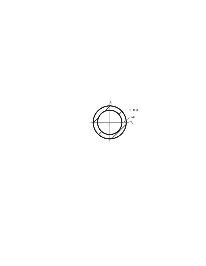
Figure 1: A 2D Landau state is represented by the ring (shaded area) of the phase-space volume $2\pi\Pi\Delta\Pi$.

As the field $B$ is raised the separation $\hbar\omega_{c}$ increases, and the quantum states are bunched together. As a result of the bunching, the density of states $\mathcal{N}(\varepsilon)$ should change periodically.

The electrons obey the Fermi-Dirac statistics. Considering a system of free electrons, we define the Helmholtz free energy $\mathcal{F}$ by

$$\mathcal{F}=N\mu-2k_{\text{B}}T\sum\ln\left[1+e^{(\mu-E_{i})/k_{\text{B}}T}\right],$$ (IV.11)

where $\mu$ is the chemical potential and the factor 2 arises from the spin degeneracy. The chemical potential $\mu$ is determined from the condition

$$\frac{\partial\mathcal{F}}{\partial\mu}=0.$$ (IV.12)

The total magnetic moment $M$ for the system can be found from

$$M=-\frac{\partial\mathcal{F}}{\partial B}.$$ (IV.13)

Equation (IV.13) is equivalent to the usual condition that the total number of the electrons, $N$, can be obtained in terms of the Fermi distribution function

$$N=2\sum_{i}f(E_{i}).$$ (IV.14)

The LL $E_{i}$ is characterized by the Landau oscillator quantum number $N_{\text{L}}$. Let us introduce the density of state

$$dW/dE\equiv\mathcal{N}(E)$$ (IV.15)

such that $\mathcal{N}(E)dE$ = the number of states having an energy between $E$ and $E+dE$. We write Eq. (IV.11) in the form

$$\mathcal{F} =N\mu-2k_{\text{B}}T\int_{0}^{\infty}dE\frac{dW}{dE}\ln\left[1+e^{(\mu-E)/k_{\text{B}}T}\right]$$

$$=N\mu-2k_{\text{B}}T\int_{0}^{\infty}dEW(E)f(E).$$ (IV.16)

The statistical weight (number) $W$ is the total number of states having energies less than

$$E=(N_{\text{L}}+1/2)\hbar\omega_{c}.$$ (IV.17)

For a fixed pair $(E,N_{\text{L}})$, the density of states is

$$dW=\frac{L_{1}L_{2}}{(2\pi\hbar)^{2}}2\pi\Pi\Delta\Pi\Theta[E-(N_{\text{L}}+1/2)\hbar\omega_{c}],$$ (IV.18)

where $\Theta(x)$ is the Heaviside step function:

$$\Theta(x)=\left\{\begin{array}[]{cl}1&\text{if }x>0\\ 0&\text{if }x<0\end{array}\right..$$ (IV.19)

We sum Eq. (IV.18) with respect to $N_{\text{L}}$ and obtain

$$W(E)=C(\hbar\omega_{c})2\sum_{N_{\text{L}}=0}^{\infty}\Theta[\varepsilon-(2N_{\text{L}}+1)\pi],$$ (IV.20)

$$C=2\pi m^{*}A(2\pi\hbar)^{-2},\quad\varepsilon\equiv 2\pi E/\hbar\omega_{c}.$$ (IV.21)

We assume a high Fermi-degeneracy such that

$$\mu\simeq\varepsilon_{\text{F}}\gg\hbar\omega_{c}.$$ (IV.22)

The sum in Eq. (IV.20) can be computed by using Poisson’s summation formula Courant

$$\sum_{n=-\infty}^{\infty}f(2\pi n)=\frac{1}{2\pi}\sum_{m=-\infty}^{\infty}\int_{-\infty}^{\infty}d\tau f(\tau)e^{-i\omega\tau}.$$ (IV.23)

We then obtain Mani_2

$$W(E)=W_{0}+W_{\text{osc}},$$ (IV.24)

$$W_{0}=A(m^{*}/\pi\hbar^{2})E$$ (IV.25)

$$W_{\text{osc}}=C\hbar\omega_{c}\frac{2}{\pi}\sum_{\nu=1}^{\infty}\frac{(-1)^{\nu}}{\nu}\sin\left(\frac{2\pi\nu E}{\hbar\omega_{c}}\right).$$ (IV.26)

The detailed calculations leading to Eqs. (IV.24)–(IV.26) are given in Appendix C. Only the first term $\nu=1$ in Eq. (IV.26) will be important in practice for weak fields

$$\varepsilon_{\text{F}}\gg\hbar\omega_{c},$$ (IV.27)

which will be shown later.

The term $W_{0}$, which is independent of $B$, gives the weight equal to that for a free electron system with no field. Note that there are no Landau-like diamagnetic terms proportional to the squared field $B^{2}$.

V SHUBNIKOV-DE HAAS OSCILLATIONS

Let us, first, consider the case with no magnetic field. We assume a uniform distribution of impurities with density $n_{I}$. We introduce a momentum distribution function $\phi(\mathbf{p},t)$, defined such that $\phi(\mathbf{p},t)d^{2}p$ gives the relative probability of finding an electron in the element $d^{2}p$ at time $t$. This function will be normalized such that

$$\frac{2}{(2\pi\hbar)^{2}}\int d^{2}p\,\phi(\mathbf{p},t)=\frac{N}{A}\equiv n,$$ (V.1)

where the factor 2 is due to the spin degeneracy.

The electric current density $\mathbf{j}$ is given in terms of $\phi(\mathbf{p},t)$ as

$$\mathbf{j}=\frac{-2e}{(2\pi\hbar)^{2}m^{*}}\int d^{2}p\,\phi(\mathbf{p},t)\mathbf{p}.$$ (V.2)

The distribution function $\phi(\mathbf{p},t)$ can be obtained by solving the Boltzmann equation for the stationary homogeneous state, dropping $t$:

$$e\mathbf{E}\boldsymbol{\cdot}\frac{\partial}{\partial\mathbf{p}}\phi(\mathbf{p})=\frac{n_{I}}{m^{*}}\int d\Omega\,I(p,\theta)[\phi(\mathbf{p}\boldsymbol{{}^{\prime}})-\phi(\mathbf{p})]p,$$ (V.3)

where $\theta$ is the scattering angle, that is, the angle between the initial momentum $\mathbf{p}$ and the final one $\mathbf{p}\boldsymbol{{}^{\prime}}$, and $I(p,\theta)$ is the differential cross section. Solving Eq. (V.3), we obtain the conductivity as Fujita_3

$$\sigma=\frac{2}{(2\pi\hbar)^{2}}\frac{e^{2}}{m^{*}}\int d^{2}p\left(-\frac{df}{dE}\right)\frac{E}{\Gamma(E)},\quad E\equiv\frac{p^{2}}{2m^{*}},$$ (V.4)

where $\Gamma$ is the energy ($E$)-dependent relaxation rate

$$\Gamma(E)=n_{I}\int d\Omega I(p,\theta)(1-\cos\theta)\frac{p}{m^{*}}.$$ (V.5)

The Fermi distribution function

$$f(E)\equiv\left[e^{\beta(E-\mu)}+1\right]^{-1}$$ (V.6)

is normalized such that

$$n =\frac{2}{(2\pi\hbar)^{2}}\int d^{2}pf(E)$$

$$=\int_{0}^{\infty}dE\nu(E)f(E),\quad\nu(E)\equiv\frac{\mathcal{N}(E)}{A},$$ (V.7)

where $\nu(E)$ is the density of states per area. We can rewrite Eq. (V.4) as

$$\sigma=\frac{e^{2}}{m^{*}}\int_{0}^{\infty}dE\nu(E)\left(-\frac{df}{dE}\right)\frac{E}{\Gamma(E)}.$$ (V.8)

The Fermi distribution function $f(E)$ drops steeply near $E=\mu$ at low temperatures: $k_{\text{B}}T\ll\varepsilon_{\text{F}}$ (Fermi energy). If the density of states varies slowly with energy $E$, then the delta-function replacement formula

$$-\frac{df}{dE}=\delta(E-\mu)$$ (V.9)

can be used. Using

$$\int_{0}^{\infty}dE\mathcal{N}(E)\left(-\frac{df}{dE}\right)E=\int_{0}^{\infty}dE\mathcal{N}(E)f(E),$$ (V.10)

and comparing Eqs. (V.8) and the Drude formula

$$\sigma=\frac{e^{2}}{m^{*}}n\frac{1}{\gamma_{0}},$$ (V.11)

we obtain

$$\frac{n}{\gamma_{0}(T)}=\int_{0}^{\infty}dE\nu(E)f(E)\frac{1}{\Gamma_{0}(E)}.$$ (V.12)

Note that the temperature dependence of the relaxation rate $\gamma_{0}(T)$ is introduced through the Fermi distribution function $f(E)$.

Let us now consider a field-dressed electron (guiding center). We assume that the dressed electron is a fermion with magnetotransport mass $M^{*}$ and charge $e$. The kinetic energy is represented by

$$\mathcal{H^{\prime}}=\frac{1}{2M^{*}}\left(\Pi_{x}^{2}+\Pi_{y}^{2}\right)\equiv\frac{1}{2M^{*}}\Pi^{2}.$$ (V.13)

We introduce a distribution function $\varphi(\mathbf{\Pi},t)$ in the $\Pi_{x}\Pi_{y}$-space normalized such that

$$\frac{2}{(2\pi\hbar)^{2}}\int d^{2}\Pi\,\varphi(\Pi_{x},\Pi_{y},t)=\frac{N}{A}=n.$$ (V.14)

The Boltzmann equation for a homogeneous stationary state of the system is

$$e(\mathbf{E}+\mathbf{v}\boldsymbol{\times}\mathbf{B})\boldsymbol{\cdot}\frac{\partial\varphi}{\partial\mathbf{\Pi}}=\int d\Omega\frac{\Pi}{M^{*}}n_{I}I(\Pi,\theta)[\varphi(\mathbf{\Pi}\boldsymbol{{}^{\prime}})-\varphi(\mathbf{\Pi})],$$ (V.15)

where $\theta$ is the scattering angle, that is, the angle between the initial and final kinetic momenta ($\mathbf{\Pi},\mathbf{\Pi}\boldsymbol{{}^{\prime}}$). In the actual experimental condition, the magnetic force term can be neglected. Assuming this condition, we obtain the same Boltzmann equation (V.3) for a field-free system except the mass difference. Hence, we obtain

$$\sigma=\frac{2e^{2}}{M^{*}(2\pi\hbar)^{2}}\int d^{2}p\frac{E}{\Gamma}\left(-\frac{df}{dE}\right).$$ (V.16)

As the field $B$ is raised, the separation $\hbar\omega_{c}$ becomes greater and the quantum states are bunched together. The statistical weight $W$ contains an oscillatory part, see Eq. (IV.26)

$$W_{\text{osc}}\propto\sin\left(\frac{2\pi\varepsilon^{\prime}}{\hbar\omega_{c}}\right),\quad\varepsilon^{\prime}=\frac{\Pi^{{}^{\prime}2}}{2m^{*}}.$$ (V.17)

Physically, the sinusoidal variations in Eq. (IV.26) arise as follows. From the Heisenberg uncertainty principle (phase space consideration) and the Pauli exclusion principle, the Fermi energy $\varepsilon_{\text{F}}$ remains approximately unchanged as the field $B$ varies. The density of states is high when $\varepsilon_{\text{F}}$ matches the $N_{\text{L}}$-th level, while it is small when $\varepsilon_{\text{F}}$ falls between neighboring LLs.

If the density of states, $\mathcal{N}(\varepsilon)$, oscillates violently in the drop of the Fermi distribution function $f(\varepsilon)\equiv\left[e^{\beta(\varepsilon-\mu)}+1\right]^{-1}$, one cannot use the delta-function replacement formula (V.9). The width of $df/d\varepsilon$ is of the order $k_{\text{B}}T$. The critical temperature $T_{c}$ below which the oscillations can be observed is

$$k_{\text{B}}T_{c}\sim\hbar\omega_{c}.$$ (V.18)

Below $T_{c}$, we may proceed as follows. Let us consider the integral

$$I=\int_{0}^{\infty}dEf(E)\sin\left(\frac{2\pi E}{\hbar\omega_{c}}\right),\quad E\equiv\frac{\Pi^{2}}{2M^{*}}.$$ (V.19)

We introduce a new variable $\zeta\equiv\beta(E-\nu)$, and extend the lower limit to $-\infty$ (low temperature limit):

$$\int_{0}^{\infty}dE\cdots\frac{1}{e^{\beta(E-\mu)}+1} =\frac{1}{\beta}\int_{-\mu\beta}^{\infty}d\zeta\cdots\frac{1}{e^{\zeta}+1}$$

$$\rightarrow\frac{1}{\beta}\int_{-\infty}^{\infty}d\zeta\cdots\frac{1}{e^{\zeta}+1}.$$ (V.20)

With the help of the integral formula

$$\int_{-\infty}^{\infty}d\zeta\frac{e^{\text{i}\alpha\zeta}}{e^{\zeta}+1}=\frac{\pi}{\text{i}\sinh\pi\alpha},$$ (V.21)

which is proved in Appendix D, we obtain from Eq. (V.19):

$$I=-\frac{\pi k_{\text{B}}T\cos(2\pi\varepsilon_{\text{F}}/\hbar\omega_{c})}{\sinh(2\pi^{2}M^{*}k_{\text{B}}T/\hbar eB)}.$$ (V.22)

Here, we used

$$M^{*}\mu(T=0)=m^{*}\varepsilon_{\text{F}},$$ (V.23)

since the Fermi momentum is the same for both dressed and undressed electrons. For very low fields, the oscillation number in the range $k_{\text{B}}T$ becomes great, and hence the sinusoidal contribution must cancel out. This effect is represented by the factor $[\sinh(2\pi^{2}M^{*}k_{\text{B}}T/\hbar eB)]^{-1}$.

We now calculate the conductivity, starting with Eq. (V.8). For the field-free case, we may use Eqs. (V.9) and (V.10) to obtain

$$\frac{n}{\gamma_{0}}=\frac{\nu(\varepsilon_{\text{F}})\varepsilon_{\text{F}}}{\Gamma_{0}(\varepsilon_{\text{F}})}.$$ (V.24)

For a finite $B$, the non-oscillatory part (background) contributes a similar amount:

$$\frac{n}{\gamma}=\frac{\nu(\varepsilon_{\text{F}})\varepsilon_{\text{F}}}{\Gamma(\varepsilon_{\text{F}})},$$ (V.25)

calculated for the dressed electrons. The oscillatory part can be calculated by using the integration formula $I$ in Eqs. (V.19) and (V.22). This part is much smaller than $\nu(\varepsilon_{\text{F}})\varepsilon_{\text{F}}/\Gamma(\varepsilon_{\text{F}})$ in Eq. (V.25), since the contribution is limited to the small energy range $k_{\text{B}}T$. It is also small by the sinusoidal cancellation. We, therefore, obtain

$$\frac{n}{\gamma} =\frac{\nu(\varepsilon_{\text{F}})\varepsilon_{\text{F}}}{\Gamma(\varepsilon_{\text{F}})}(1+\phi),$$ (V.26)

$$\phi \equiv\frac{\pi k_{\text{B}}T}{\varepsilon_{\text{F}}}\frac{\cos(2\pi\varepsilon_{\text{F}}/\hbar\omega_{c})}{\sinh(2\pi^{2}M^{*}k_{\text{B}}T/\hbar eB)}.$$ (V.27)

Strictly speaking, the contribution of the terms with $\nu=2,3,\cdots$ in the sum $W_{\text{osc}}$ in Eq. (IV.26) should be added. But this contribution, which carries $[\sinh(2\pi^{2}\nu M^{*}k_{\text{B}}T/\hbar eB)]^{-1}$, is small since

$$\sinh(2\pi^{2}M^{*}k_{\text{B}}T/\hbar eB)\gg 1.$$ (V.28)

In the present theory, the two masses $m^{*}$ and $M^{*}$ are introduced naturally corresponding to the two physical processes: the cyclotron motion of the electron and the guiding center motion of the dressed electron. The dressed electron is the same entity as the c-fermion with two fluxons in the QHE theory.

In summary, the magnetoconductivity $\sigma(B)$, given by Eq. (V.16), may be written out as

$$\sigma=\frac{e^{2}}{M^{*}}\frac{n}{\gamma}=\frac{e^{2}}{M^{*}}\frac{\nu(\varepsilon_{\text{F}})\varepsilon_{\text{F}}}{\Gamma(\varepsilon_{\text{F}})}(1+\phi).$$ (V.29)

In contrast, the conductivity $\sigma_{0}$ at zero field is

$$\sigma_{0}=\frac{e^{2}}{m^{*}}\frac{n}{\gamma_{0}}=\frac{e^{2}}{m^{*}}\frac{\nu(\varepsilon_{\text{F}})\varepsilon_{\text{F}}}{\Gamma_{0}(\varepsilon_{\text{F}})},$$ (V.30)

where we have assumed that the Fermi energy $\varepsilon_{\text{F}}$ remains the same for both cases. We note that the magnetoconductivity $\sigma$ does not approach the conductivity $\sigma_{0}$ in the low field limit. In fact, we obtain in this limit ($\phi=0$):

$$\sigma-\sigma_{0}=e^{2}n\left(\frac{1}{M^{*}\gamma}-\frac{1}{m^{*}\gamma_{0}}\right).$$ (V.31)

The difference arises from the carrier difference.

If the “decay” rate $\delta=2\pi^{2}M^{*}k_{\text{B}}T/\hbar e$ defined through

$$\sinh(\delta/B)\equiv\sinh(2\pi^{2}M^{*}k_{\text{B}}T/\hbar eB)$$ (V.32)

is measured carefully, the magnetotransport mass $M^{*}$ can be obtained directly through

$$M^{*}=e\hbar\delta/(2\pi^{2}k_{\text{B}}T).$$ (V.33)

Mani measured the SdH oscillations in GaAs/AlGaAs Mani_2 , Fig. 1, $T=0.7$ K. His data are reproduced in Fig. 2.

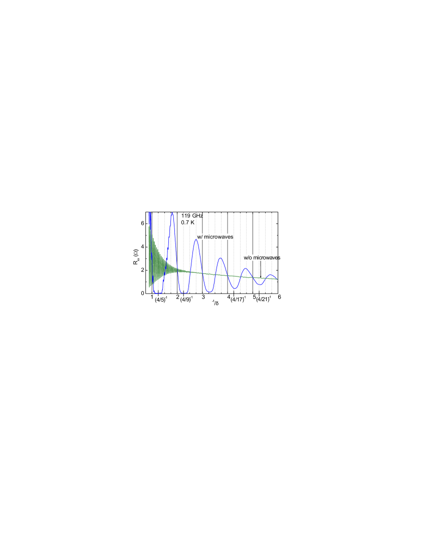
Figure 2: The resistance $R_{xx}$ versus the reduced inverse magnetic field, $B^{\prime-1}$. See Mani Mani_2 for the actual reduction. The number $N$ in the abscissas is the intersection number between the curves with (w/) and without (w/o) microwaves.

Clearly, we see the diagonal resistance $R_{xx}$ linearly decreasing with $B^{-1}$ in the low field limit. For high purity samples at very low temperature ($\sim 0.7$ K), the impurity and phonon scatterings are negligible. By the energy-time uncertainty principle the dressed electron can spend a short time at the upper LL and come back to the ground LL with a different guiding center, which causes a guiding center jump. We assume that the relaxation rate $\gamma$ is the natural linewidth arising from the LL separation divided by $\hbar$, that is, the cyclotron frequency $\omega_{c}$:

$$\gamma=\omega_{c}=eB/m^{*}.$$ (V.34)

This generates the desired $B^{-1}$ dependence for $R_{xx}$.

We fitted Mani’s data in Fig. 2 with

$$R_{xx}=A+Bx+\frac{[E\cos(2\pi Cx)+F]x}{\sinh(Dx)},$$ (V.35)

where $A=2.3$, $B=-0.18$, $C=23.0$, $D=3.1$, $E=22.0$, and $F=7.0$. The fits agree with the data within the experimental errors. Using $Dx=\delta/B$, we obtain

$$M^{*}=0.30\,m_{e},$$ (V.36)

where $m_{e}$ is the gravitational electron mass. If $m^{*}=0.067\,m_{e}$, then $M^{*}/m^{*}=4.5$. These are reasonable numbers.

The relaxation rate $\gamma=\Gamma(\varepsilon_{\text{F}})$ can now be obtained through Eq. (V.11) with the measured magnetoconductivity. All electrons, not just those excited electrons near the Fermi surface, are subject to the electric field. Hence, the carrier density $n$ appearing in Eq. (V.29) is the total density $n$ of the dressed electrons. This $n$ also appears in the Hall resistivity expression

$$\rho_{\text{H}}\equiv\frac{E_{\text{H}}}{j}=\frac{v_{d}B}{env_{d}}=\frac{B}{en},$$ (V.37)

where the Hall effect condition:

$$E_{\text{H}}=v_{d}B,\quad v_{d}=\text{drift velocity}$$ (V.38)

was used.

The dressed electrons are there whether the system is probed in equilibrium or in nonequilibrium as long as the system is subjected to a magnetic field. Hence their presence can be checked by measuring the susceptibility or the heat capacity of the system. All (dressed) electrons are subject to the magnetic field, and hence the magnetic susceptibility $\chi$ is proportional to the carrier density $n$ although the $\chi$ depends critically on the Fermi surface. We shall briefly discuss the magnetic moment and susceptibility.

The magnetization $\mathcal{M}$, that is, the total magnetic moment per unit area, can be obtained from

$$\mathcal{M}=-\frac{\partial\mathcal{F}}{\partial B}.$$ (V.39)

Using Eqs. (IV.12) and (IV.22), we obtain the magnetization $\mathcal{M}$ for the quasi-free electrons Fujita_3

$$\mathcal{M}=2n\frac{\mu_{\text{B}}^{2}}{\varepsilon_{\text{F}}}\bigg{[}1-\left(\frac{\varepsilon_{\text{F}}}{\mu_{\text{B}}B}\right)\frac{k_{\text{B}}T}{\varepsilon_{\text{F}}}\left(\frac{m^{*}}{M^{*}}\right)\\ \times\frac{\cos(2\pi\varepsilon_{\text{F}}/\hbar\omega_{c})}{\sinh(2\pi^{2}Mk_{\text{B}}T/\hbar eB)}\bigg{]},$$ (V.40)

where $\mu_{\text{B}}$ is the Bohr magneton. The magnetic susceptibility $\chi$ is defined by the ratio

$$\chi\equiv\frac{\mathcal{M}}{B}.$$ (V.41)

VI TRANSPORT DIAMOND AND ZERO CURRENT ANOMALY

We are now ready to discuss the TD and ZCA observed by Studenikin et al. Studenikin . Ref. Studenikin , Fig. 1 is reproduced in Fig. 3.

Figure 3: The differential resistance $r$ of an InGaAs/InP Hall bar (width = $100\,\mu$m) at different DC values, $T=270$ mK. All curves except at $I_{\text{DC}}=0$ are shifted vertically by $0.25$ k$\Omega$ for clarity.

The outstanding features are:

1. The differential resistance $r\equiv dV/dI$ exhibit the SdH oscillations for higher DC, $I_{\text{DC}}=50\,\mu$A. The envelope of the SdH oscillations become smaller for weaker magnetic fields.

2. The background differential resistance for the SdH is zero.

3. The flat minima present at $I_{\text{DC}}=0$ indicate a QHE. The flat minimum means a zero resistance

   $$R\equiv V/I=0.$$ (VI.1)

4. The SdH maxima and the QHE minima both have the right-left symmetry with varying magnetic fields.

5. As the DC increases, the SdH maxima progressively become the QHE minima.

Our interpretation is as follows.

1. The SdH oscillations are described by formula (V.27). The oscillations are sinusoidal:

   $$\cos(2\pi\varepsilon_{\text{F}}/\hbar\omega_{c})=\cos(2\pi m^{*}\varepsilon_{\text{F}}/\hbar eB),$$ (VI.2)

   and the envelope is represented by

   $$\frac{\pi k_{\text{B}}T}{\varepsilon_{\text{F}}}\frac{1}{\sinh(2\pi^{2}M^{*}k_{\text{B}}T/\hbar eB)}.$$ (VI.3)

   The cyclotron mass $m^{*}$ appears in Eq. (VI.2) and the magnetotransport mass $M^{*}$ enters in Eq. (VI.3). The two masses ($m^{*},M^{*}$) correspond to the cyclotron motion and the guiding center motion, respectively. We avoid the use of a Dingle temperature Jain .

2. The background resistance $\langle R\rangle$ averaged over the field $B$ is zero:

   $$\langle R\rangle\equiv\left\langle\frac{V}{I}\right\rangle=0.$$ (VI.4)

   This behaviour is in agreement with formula (V.26). It arises from the fact that there is no Landau-like term proportional to the squared magnetic field $B^{2}$ in the statistical weight $W$ in 2D, see Eq. (IV.24). (There is no Landau diamagnetism in 2D in contrast to the 3D case.)

3. The flat minimum meaning zero resistance $R=0$, indicates the existence of a superconducting state. The superconducting state is stable with an energy gap. The supercurrents run with no scatterings by impurities and phonons. As is well known, the magnetic field is detrimental to the superconducting state. If the excess magnetic field $B^{*}$ relative to the center field of the horizontal stretch exceeds a critical field, then the superconductivity is destroyed. The microscopic origin of this effect was explained in section 2. Briefly, the supercurrent is composed of the positively and negatively charged pairon-currents. The excess magnetic field $B^{*}$ generates oppositely directed forces and breaks up $\pm$ pairons (Cooper pairs).

4. The magnetic field energy is quadratic in the excess field $B^{*}$, see Eq. (II.19), which explains the right-left symmetry of the destroyment of the superconducting state.

5. The integer QHE occurring at the LL occupation numbers $\nu=P=1,2,\dots$, have the quantized magnetic fluxes:

   $$BA=\frac{1}{P}\Phi_{0}N_{\phi_{1}}=\frac{1}{P}\left(\frac{h}{e}\right)N_{\phi_{1}},$$ (VI.5)

   where $N_{\phi_{1}}$ is the fluxon number at $\nu=P=1$. Hence the QHE has maxima at

   $$B=\frac{1}{P}\left(\frac{h}{e}\right)n_{\phi_{1}},\quad n_{\phi_{1}}\equiv\frac{N_{\phi_{1}}}{A}.$$ (VI.6)

   Equations (V.27) and (V.29) indicate that the resistivity $r$ has minima when

   $$\cos(2\pi\varepsilon_{\text{F}}/\hbar\omega_{c})=1,$$ (VI.7)

   whose solutions are

   $$\frac{2\pi\varepsilon_{\text{F}}}{\hbar\omega_{c}}=2\pi Q,\quad Q=1,2,\dots.$$ (VI.8)

   We use $\omega_{c}=eB/m^{*}$, $\varepsilon_{\text{F}}=p_{\text{F}}^{2}/2m^{*}$, $2\pi p_{\text{F}}^{2}=n_{e}e$, and solve Eq. (VI.8) for $B$ and obtain

   $$B=\frac{h}{e}\frac{1}{Q}n_{e_{1}},$$ (VI.9)

   where $n_{e_{1}}$ is the electron density at $\nu=1$. From Eq. (II.17), we obtain

   $$n_{e_{1}}=n_{\phi_{1}}.$$ (VI.10)

   Both $P$ and $Q$ are positive integers. Hence we find from Eqs. (VI.6) and (VI.9) that the integer QHE maxima and the SdH minima occur precisely at the same magnetic fields $B$. Thus, the QHE minima progressively turn into the SdH maxima with increasing DC.

Fig. 2, Ref. Studenikin is reproduced in Fig. 4.

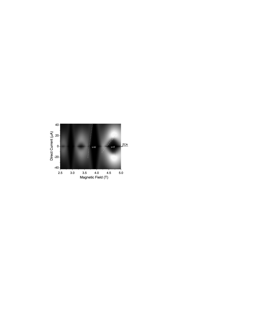
Figure 4: The differential resistance $r$ of an InGaAs/InP Hall bar ($w=100\,\mu$m) is plotted versus magnetic field and DC. The ZCA position is indicated by arrow.

The differential resistance $r\equiv dV/dI$ is plotted versus magnetic field (T) and direct current ($\mu$ A). Diamond-shaped regions near SdH minima are called transport diamonds (TD).

Our interpretation of the TD is a break-down of the superconducting QH state due to the excess magnetic field and the direct current. The direct current by itself generates a magnetic field, which is detrimental to the superconducting state.

Fig. 5 is reproduced after Ref. Studenikin , Fig. 3.

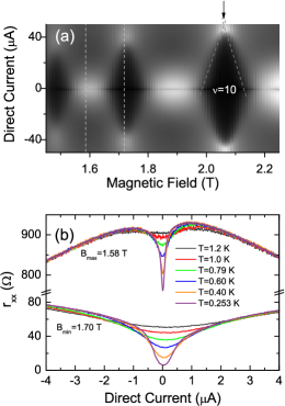
Figure 5: (a) The differential resistance of an InGaAs/InP Hall bar ($w=100\,\mu$m), $T=300$ mK, is plotted versus magnetic field and DC; (b) the ZCA at two magnetic fields ($1.58$ T, $1.70$ T) indicated by vertical dashed lines in (a) for different temperatures.

In (a) transport diamonds are shown, which are similar to those in Fig. 2. The temperature-dependence of the differential resistance is shown in (b) in the range ($0.253$–$1.2$ K).

The sharp dip in $r$ vs. DC near $\text{DC}=0$ observed in Fig. 3 and Fig. 5(a) is called the ZCA, the narrow horizontal line indicated by an arrow in Fig. 3. Its temperature behavior at $B=1.58$ T and $B=1.70$ T is shown in Fig. 5(b).

The original authors Studenikin suspect that the origin of the ZCA arises from the Coulomb gap in the one particle density of states of interacting electrons. We propose a differing interpretation:

Let us consider the case of the SdH at $B=1.58$ T, the top figure in Fig. 5(b). At the low temperatures $T=(0.253$–$1.2)$ K, the optical phonon population given by the Plank distribution function can be approximated by the Boltzmann distribution function:

$$n_{\text{ph}}=\frac{1}{e^{\beta\varepsilon_{0}}-1}\cong e^{-\varepsilon_{0}/k_{\text{B}}T},$$ (VI.11)

where $\varepsilon_{0}$ is the longitudinal optical phonon energy (assumed constant) and $k_{\text{B}}$ the Boltzmann constant. The temperature dependence is exponential. The phonon population $n_{\text{ph}}$ is rapidly changing with temperature and dominates. The resistance $R$ is proportional to the electron-phonon scattering rate $\gamma_{\text{ph}}$:

$$R\equiv\sigma^{-1}\propto\gamma_{\text{ph}}=n_{\text{ph}}v_{\text{ph}}\mathcal{A},$$ (VI.12)

where $v_{\text{ph}}$ is the phonon speed, $\mathcal{A}$ the electron-phonon scattering cross section, and $n_{\text{ph}}$ the phonon population given in Eq. (VI.11).

Studenikin et al. Studenikin observed that the temperature dependence of the ZCA follows the Arrhenius law:

$$\gamma\propto e^{-\varepsilon_{A}/k_{\text{B}}T}$$ (VI.13)

with the activation energy

$$\varepsilon_{A}/k_{\text{B}}=1.3\,\text{K}.$$ (VI.14)

This value may correspond to the optical phonon energy $\varepsilon_{0}$:

$$\varepsilon_{A}=\varepsilon_{0}.$$ (VI.15)

This finding supports our view that the temperature dependence of the ZCA arises from the electron-phonon scattering.

We next consider the ZCA for the QHE at $B=1.70$ T. This ZCA is also temperature-dependent. As the temperature decreases from $1.2$ K to $0.253$ K, the negative peak decreases in magnitude and its width becomes narrower. In the QHE under radiation, a supercurrent due to moving pairons condensed run in the upper (excited) channel and a normal current due to electrons run in the base channel. The resistance of the normal current is proportional to the electron-phonon scattering rate $\gamma_{\text{ph}}$, as shown in Eq. (VI.6). Then, the phonon population approximately decreases exponentially at low temperatures (below $1.2$ K). Thus the resistance decreases as the temperature $T$ is lowered, which explains the observed temperature dependence.

The QHE at zero DC is destroyed either by increasing excess magnetic fields or by increasing DC-induced magnetic fields. But the ZCA indicates the destroyment is sharper for the case of increasing DC. This difference should arise from the direction of the magnetic field. The DC running along the sample length is likely to be inhomogeneous, stronger at the outer edge. Then the superconductivity is destroyed at the edges first according to Silsbeeb rule. On the other hand, the applied magnetic field alone should keep the current homogeneous.

Studenikin et al. Studenikin observed essentially same TD and ZCA in heterojunction GaAs/AlGaAs. In particular, the QHE minima progressively turn to the SdH maxima as DC increases, and the ZCA is sharp near $\text{DC}=0$. The same theory applies here. The authors thank Dr. S. Studenikin for enlightening discussions.

Appendix A DERIVATION OF EQS. (II.5) AND (II.6)

Dropping the “holes” from the Hamiltonian $\mathcal{H}$ in Eq. (II.2), we obtain

$$\mathcal{H}_{c}= \sum_{\mathbf{k}}\sum_{\mathbf{q}}\left(\varepsilon_{|\mathbf{k}\boldsymbol{+}\mathbf{q}/2|}+\varepsilon_{|\boldsymbol{-}\mathbf{k}\boldsymbol{+}\mathbf{q}/2|}^{(3)}\right)B_{\mathbf{kq}}^{\dagger}B_{\mathbf{kq}}$$

$$-v_{0}\sideset{}{{}^{\prime}}{\sum}_{\mathbf{q}}\sideset{}{{}^{\prime}}{\sum}_{\mathbf{k}}\sideset{}{{}^{\prime}}{\sum}_{\mathbf{k}\boldsymbol{{}^{\prime}}}B_{\mathbf{k}\boldsymbol{{}^{\prime}}\mathbf{q}}^{\dagger}B_{\mathbf{kq}},$$ (A.1)

where we suppressed the “electron” and spin indices. Using the anticommutation rules (II.6), we obtain

$$\left[\mathcal{H}_{c},B_{\mathbf{kq}}^{\dagger}\right]= \left(\varepsilon_{|\mathbf{k}\boldsymbol{+}\mathbf{q}/2|}+\varepsilon_{|\boldsymbol{-}\mathbf{k}\boldsymbol{+}\mathbf{q}/2|}^{(3)}\right)B_{\mathbf{kq}}^{\dagger}$$

$$\mbox{}-v_{0}\sideset{}{{}^{\prime}}{\sum}_{\mathbf{k}\boldsymbol{{}^{\prime}}}B_{\mathbf{k}\boldsymbol{{}^{\prime}}\mathbf{q}}^{\dagger}\left(1-n_{\mathbf{k}\boldsymbol{+}\mathbf{q}/2}-n_{\boldsymbol{-}\mathbf{k}\boldsymbol{+}\mathbf{q}/2}^{(3)}\right).$$ (A.2)

The Hamiltonian $\mathcal{H}_{c}$ is bilinear in $(B,B^{\dagger})$, and can therefore be diagonalized exactly:

$$\mathcal{H}_{c}=\sum_{\mu}w_{\mu}\phi_{\mu}^{\dagger}\phi_{\mu},$$ (A.3)

where $w_{\mu}$ is the energy and $\phi_{\mu}$ the annihilation operator. We multiply Eq. (A.2) by $\phi_{\mu}$ from the right, take a grand canonical ensemble average, denoted by angular brackets, and get

$$w_{\mu}\Psi_{\mu}(\mathbf{k,q})=\left(\varepsilon_{|\mathbf{k}\boldsymbol{+}\mathbf{q}/2|}+\varepsilon_{|\boldsymbol{-}\mathbf{k}\boldsymbol{+}\mathbf{q}/2|}^{(3)}\right)\Psi_{\mu}(\mathbf{k,q})\\ -\frac{v_{0}}{(2\pi\hbar)^{2}}\int^{\prime}d^{2}k^{\prime}\Psi_{\mu}(\mathbf{k^{\prime},q})\\ \times\Big{\langle}1-f_{\text{F}}\left(\varepsilon_{|\mathbf{k}\boldsymbol{{}^{\prime}+}\mathbf{q}/2|}\right)-f_{\text{F}}\left(\varepsilon_{|\boldsymbol{-}\mathbf{k}\boldsymbol{{}^{\prime}+}\mathbf{q}/2|}^{(3)}\right)\Big{\rangle},$$ (A.4)

where $\langle n_{p}\rangle=f_{\text{F}}(\varepsilon_{p})$ is the Fermi distribution function. The reduced wavefunction

$$\Psi_{\mu}(\mathbf{k,q})\equiv\left\langle B_{\mathbf{kq}}^{\dagger}\phi_{\mu}\right\rangle=\langle\boldsymbol{\mu}|\hat{n}|\mathbf{k,q}\rangle$$ (A.5)

can be regarded as the mixed representation of the reduced density operator $\hat{n}$ defined through $\langle\mathbf{k}\boldsymbol{{}^{\prime}},\mathbf{q}\boldsymbol{{}^{\prime}}|\hat{n}|\mathbf{k,q}\rangle\equiv\left\langle B_{\mathbf{k,q}}^{\dagger}B_{\mathbf{k}\boldsymbol{{}^{\prime}},\mathbf{q}\boldsymbol{{}^{\prime}}}\right\rangle$. The fc-boson energy $w_{\mu}$ can be specified by $(N_{\text{L}},q)$, and it will be denoted by $w_{q}$ since it is $N_{\text{L}}$-independent. As $T\rightarrow 0$, $f_{\text{F}}(\varepsilon_{p})\rightarrow 0$. Dropping the fluxon energy and replacing $\mathbf{q}/2$ by $\mathbf{q}$, we obtain Eq. (II.5). We solve this equation, assuming $\varepsilon_{\text{F}}\gg\hbar\omega_{\text{D}}$. Using a Taylor series expansion, we obtain Eq. (II.6) to the linear in $q$.

Appendix B DERIVATION OF EQ. (II.7)

The BEC occurs when the chemical potential $\mu$ vanishes at a finite $T$. The critical temperature $T_{c}$ can be determined from

$$n=(2\pi\hbar)^{-2}\int d^{2}p\left[e^{\beta_{c}\varepsilon}-1\right]^{-1},\quad\beta_{c}\equiv(k_{\text{B}}T_{c})^{-1}.$$ (B.1)

After expanding the integrand in powers of $e^{-\beta_{c}\varepsilon}$ and using $\varepsilon=cp$, we obtain

$$n=1.654(2\pi)^{-1}(k_{\text{B}}T_{c}/\hbar c)^{2},$$ (B.2)

yielding Eq. (II.7).

Appendix C STATISTICAL WEIGHT FOR THE LANDAU STATES

The statistical weight $W$ for the Landau states in 2D will be calculated in this appendix. We write the sum in Eq. (II.16) as

$$2\sum_{n=0}^{\infty}\Theta(\epsilon-(2n+1)\pi)=\Theta(\epsilon-\pi)+\psi(\epsilon;0),$$ (C.1)

$$\psi(\epsilon;x)\equiv\sum_{n=-\infty}^{\infty}\Theta(\epsilon-\pi-2\pi|n+x|).$$ (C.2)

Note that $\psi(\epsilon;x)$ is periodic in $x$ and can therefore be expanded in a Fourier series. After the Fourier expansion, we set $x=0$ and obtain Eq. (C.1). By taking the real part (Re) of Eq. (C.1) and using Eq. (IV.20), we obtain

$$\text{Re\{Equation\ \eqref{eq:siE_as}\}}=\frac{1}{\pi}\int_{0}^{\infty}d\tau\Theta(\epsilon-\tau)\\ +\frac{2}{\pi}\sum_{\nu=1}^{\infty}(-1)^{\nu}\int_{0}^{\infty}d\tau\Theta(\epsilon-\tau)\cos\nu\tau,$$ (C.3)

where we assumed $\epsilon\equiv 2\pi E/\hbar\omega_{c}\gg 1$ and neglected $\pi$ against $\epsilon$. The integral in the first term in Eq. (C.3) yields $\epsilon$. The integral in the second term is

$$\int_{0}^{\infty}d\tau\Theta(\epsilon-\tau)\cos\nu\tau=\frac{1}{\nu}\sin\nu\epsilon.$$ (C.4)

We then obtain

$$\text{Re\{Equation\ \eqref{eq:siE_as}\}}=\frac{1}{\pi}\epsilon+\frac{2}{\pi}\sum_{\nu=1}^{\infty}\frac{(-1)^{\nu}}{\nu}\sin\nu\epsilon.$$ (C.5)

Using Eqs. (IV.20) and (C.5), we obtain

$$W(E) =W_{0}+W_{\text{osc}}$$

$$=C\hbar\omega_{c}\left(\frac{\epsilon}{\pi}\right)+C\hbar\omega_{c}\frac{2}{\pi}\sum_{\nu=1}^{\infty}\frac{(-1)^{\nu}}{\nu}\sin\left(\frac{2\pi\nu E}{\hbar\omega_{c}}\right).$$ (C.6)

Appendix D DERIVATION OF EQ. (V.21)

Let us consider an integral on the real axis

$$I(y,\alpha,R)=\int_{-R}^{R}dx\frac{e^{\text{i}\alpha(x+\text{i}y)}}{e^{z}+1},\quad z=x+\text{i}y\text{ and }\alpha,R>0.$$ (D.1)

We add an integral over a semicircle of radius $R$ in the upper $z$-plane to form an integral over a closed contour. We then take the limit: $R\rightarrow\infty$. The integral over the semicircle vanishes in this limit if $\alpha>0$. The integral on the real axis, $I(y,\alpha,\infty)$, becomes the desired integral in Eq. (V.21). The integral over the closed contour can be evaluated by using the residue theorem. Note that $(e^{z}+1)^{-1}$ has simple poles at $z=\pi\text{i},3\pi\text{i},\dots,(2n-1)\pi\text{i},\dots.$ We may use the following formula valid for a simple pole at $z=z_{j}$:

$$\text{Res}\{p(z)/q(z),z_{j}\}=p(z_{j})/q^{\prime}(z_{j}),$$ (D.2)

where $p(z)$ is analytic at $z=z_{j}$, and the symbol Res means a residue. We then obtain

$$I(\alpha,\infty) =2\pi\text{i}\cdot\sum_{n=1}^{\infty}\text{Res}\left\{\frac{e^{\text{i}\alpha z}}{e^{z}+1},z_{n}=(2n-1)\pi\text{i}\right\}$$

$$=2\pi\text{i}\cdot\sum_{n=1}^{\infty}\frac{e^{\text{i}\alpha[(2n-1)\pi\text{i}]}}{e^{(2n-1)\pi\text{i}}}=-2\pi\text{i}\frac{e^{-\alpha\pi}}{1-e^{-2\alpha\pi}}$$

$$=\frac{\pi}{\text{i}}\frac{1}{\sinh\alpha\pi}.$$ (D.3)

References

- (1) S.A. Studenikin, G. Granger, A. Kam, A.S. Sachrajda, Z.R. Wasilewski, and P.J. Poole, arXiv:1012.0043v1 [cond-mat.mes-hall] (2010).
- (2) S.C. Zhang, T.H. Hansson, and S. Kivelson, Phys. Rev. Lett. 62, 82 (1989).
- (3) S. Fujita and Y. Okamura, Phys. Rev. B69, 155313 (2004); S. Fujita, Y. Tamura, and A. Suzuki, Mod. Phys. Lett. B 15, 817 (2001); S. Fujita, K. Ito, Y. Kumek, and Y. Okamura, Phys. Rev. 70, 075304 (2004).
- (4) Z.F. Ezawa, Quantum Hall Effect (World Scientific, Singapore, 2000); see also R.E. Prange and S.M. Girvin, eds., Quantum Hall Effect (Springer-Verlag, New York, 1990); B.I. Halperin, P.A. Lee, and N. Read, Phys. Rev. B47, 7312 (1993); M. Janssen, O. Viehweger, V. Fastenrath, and J. Hajdu, Introduction to the Theory of the Integer Quantum Hall Effect (VCH, Weinbeim, Germany, 1994).
- (5) J.K. Jain, Phys. Rev. Lett. 63, 199 (1989), Phys. Rev. B40, 8079 (1989); ibid, 41, 7653 (1990); Surf. Sci. 263, 65 (1992).
- (6) L.W. Shubnikov and W.J. de Haas, Proc. Netherlands Royal Acad. Sci., 33, 130 and 163 (1932).
- (7) W.J. de Haas and P.M. van Alphen, Leiden Comm., 208d, 211a (1930); Leiden Comm., 220d (1932).
- (8) R.B. Dingle, Proc. Roy. Soc. A211, 500 (1952).
- (9) S. Fujita, S. Horie, A. Suzuki, and D.L. Morabito, Ind. J. PAP, 44, 850 (2006).
- (10) S. Fujita and D.L. Morabito, Mod. Phys. Lett. B 12, 753 (1998).
- (11) P. Ehrenfest and J.R. Oppenheimer, Phys. Rev. 37, 311 (1931); H.A. Bethe and R. Jackiw, Intermediate Quantum Mechanics, 2nd ed. (Benjamin, New York, 1968), p. 23.
- (12) J. Bardeen, L.N. Cooper, and J.R. Schrieffer, Phys. Rev. 108, 1175 (1957).
- (13) S. Fujita and K. Ito, Quantum Theory of Conducting Matter (Springer, New York, 2007), pp. 119–122, pp. 78–82, pp. 144–145.
- (14) S. Fujita, J.H. Kim, K. Ito, and M. De Llano, Internat. J. Mod. Phys. B 23, 4129 (2009).
- (15) S. Fujita and S. Godoy, Quantum Statistical Theory of Superconductivity (Plenum, New York, 1996), pp. 184–186, pp. 202–204.
- (16) R.G. Mani et al., Nature, 420, 646 (2002).
- (17) M.A. Zudov et al., Phys. Rev. Lett. 90, 046807 (2003).
- (18) R. Courant and D. Hilbert, Methods of Mathematical Physics, vol. 1 (Interscience-Wiley, New York, 1953), pp. 76–77.
- (19) R.G. Mani, Physica E, 22, 1 (2004).