First Measurement of $\phi_{3}$ with a Binned Model-independent Dalitz Plot Analysis of $B^{\pm}\to DK^{\pm}$, $D\to K^{0}_{S}\pi^{+}\pi^{-}$ Decay

Abstract

We present the first measurement of the angle $\phi_{3}$ of the unitarity triangle using a binned model-independent Dalitz plot analysis technique of $B^{\pm}\to DK^{\pm}$, $D\to K^{0}_{S}\pi^{+}\pi^{-}$ decay chain. The method is based on the measurement of parameters related to the strong phase of $D\to K^{0}_{S}\pi^{+}\pi^{-}$ amplitude performed by the CLEO collaboration. The analysis uses full data set of $772\times 10^{6}$ $B\overline{B}$ pairs collected by the Belle experiment at $\Upsilon(4S)$ resonance. We obtain $\phi_{3}=(77.3^{+15.1}_{-14.9}\pm 4.2\pm 4.3)^{\circ}$ and the suppressed amplitude ratio $r_{B}=0.145\pm 0.030\pm 0.011\pm 0.011$. Here the first error is statistical, the second is experimental systematic uncertainty, and the third is the error due to precision of strong phase parameters obtained by CLEO. This result is preliminary.

I Introduction

The angle $\phi_{3}$ (also denoted as $\gamma$) is one of the least well-constrained parameters of the Unitarity Triangle. The theoretical uncertainties in $\phi_{3}$ determination are expected to be negligible, and the main difficulty in its measurement is a very low probability of the decays involved.

The measurement that currently dominates the $\phi_{3}$ sensitivity uses $B^{\pm}\to DK^{\pm}$ decay with the neutral $D$ meson decaying to 3-body final state such as $K^{0}_{S}\pi^{+}\pi^{-}$ giri ; binp_dalitz . The weak phase $\phi_{3}$ appears in the interference between $b\to c\bar{u}s$ and $b\to u\bar{c}s$ transitions and can be measured in the Dalitz plot analysis of the $D$ decay. This method requires the knowledge of the amplitude of $D^{0}\to K^{0}_{S}\pi^{+}\pi^{-}$ decay including its complex phase. The amplitude is obtained from the model that involves isobar and K-matrix descriptions of the decay dynamics, and thus results in the model uncertainty of the $\phi_{3}$ measurement. In the latest model-dependent Dalitz plot analyses performed by BaBar and Belle, this uncertainty ranges from 3^∘ to 9^∘ babar_gamma_1 ; babar_gamma_2 ; babar_gamma_3 ; belle_phi3_1 ; belle_phi3_2 ; belle_phi3_3 .

The method to eliminate the model uncertainty using the binned Dalitz plot analysis has been proposed by Giri et al. giri . The information about the strong phase in $D^{0}\to K^{0}_{S}\pi^{+}\pi^{-}$ decay is obtained from the decays of quantum-correlated $D^{0}$ pairs produced in $\psi(3770)\to D^{0}\overline{D}{}^{0}$ process. As a result, the model uncertainty is substituted by the statistical error related to the precision of strong phase parameters. The method has been further developed in modind2006 ; modind2008 where the experimental feasibility of the method has been shown and the analysis procedure has been proposed to optimally use the available $B$ decays and correlated $D^{0}$ pairs. Recently, the measurement of strong phase in $D^{0}\to K^{0}_{S}\pi^{+}\pi^{-}$ and $D^{0}\to K^{0}_{S}K^{+}K^{-}$ decays has been performed by CLEO collaboration cleo_1 ; cleo_2 . In this paper, we report the first measurement of $\phi_{3}$ with the model-independent Dalitz plot analysis of $D\to K^{0}_{S}\pi^{+}\pi^{-}$ decay from the mode $B^{\pm}\to DK^{\pm}$, based on a 711 fb^-1 data sample (corresponding to $772\times 10^{6}$ $B\overline{B}$ pairs) collected by the Belle detector at the KEKB asymmetric $e^{+}e^{-}$ factory using the CLEO measurement. These results are preliminary.

II The model-independent Dalitz plot analysis technique

The amplitude of the $B^{+}\to DK^{+}$, $D\to K^{0}_{S}\pi^{+}\pi^{-}$ decay is given by the interference of $B^{+}\to\overline{D}{}^{0}K^{+}$ and $B^{+}\to D^{0}K^{+}$ amplitudes:

$$A_{B}=\overline{A}+r_{B}e^{i(\delta_{B}+\phi_{3})}A\,,$$ (1)

where $\overline{A}=\overline{A}(m^{2}_{K_{S}\pi^{+}},m^{2}_{K_{S}\pi^{-}})\equiv\overline{A}(m^{2}_{+},m^{2}_{-})$ is the amplitude of the $\overline{D}{}^{0}\to K^{0}_{S}\pi^{+}\pi^{-}$ decay, $A=A(m^{2}_{+},m^{2}_{-})$ is the amplitude of the $D^{0}\to K^{0}_{S}\pi^{+}\pi^{-}$ decay ($A(m^{2}_{+},m^{2}_{-})=\overline{A}(m^{2}_{-},m^{2}_{+})$ in the case of $CP$ conservation in $D$ decay), $r_{B}$ is the ratio of the absolute values of the two interfering amplitudes, and $\delta_{B}$ is the strong phase difference between them. The Dalitz plot density of the $D$ decay from $B^{+}\to DK^{+}$  is given by

$$\begin{split}P_{B}=|A_{B}|^{2}=&|\overline{A}+r_{B}e^{i(\delta_{B}+\phi_{3})}A|^{2}=\\ &\overline{P}+r_{B}^{2}P+2\sqrt{P\overline{P}}(x_{+}C+y_{+}S)\,,\end{split}$$ (2)

where

$$x_{+}=r_{B}\cos(\delta_{B}+\phi_{3})\,;\;\;\;y_{+}=r_{B}\sin(\delta_{B}+\phi_{3})\,.$$ (3)

The functions $C=C(m^{2}_{+},m^{2}_{-})$ and $S=S(m^{2}_{+},m^{2}_{-})$ are the cosine and sine of the strong phase difference $\delta_{D}=\arg\overline{A}-\arg A$ between the $\overline{D}{}^{0}\to K^{0}_{S}\pi^{+}\pi^{-}$ and $D^{0}\to K^{0}_{S}\pi^{+}\pi^{-}$ amplitudes:

$$C=\cos\delta_{D}(m^{2}_{+},m^{2}_{-})\,;\;\;\;S=\sin\delta_{D}(m^{2}_{+},m^{2}_{-})\,.$$ (4)

The equations for the charge-conjugate mode $B^{-}\to DK^{-}$ are obtained with the substitution $\phi_{3}\rightarrow-\phi_{3}$ and $A\leftrightarrow\overline{A}$; the corresponding parameters of the admixture of the suppressed amplitude are

$$x_{-}=r_{B}\cos(\delta_{B}-\phi_{3})\,;\;\;\;y_{-}=r_{B}\sin(\delta_{B}-\phi_{3})\,.$$ (5)

Using both $B$ charges, one can obtain $\phi_{3}$ and $\delta_{B}$ separately.

Up to this point, the description of the model-dependent and model-independent techniques is the same. The model-dependent analysis deals directly with the Dalitz plot density, and the functions $C$ and $S$ are obtained from model assumptions in the fit of the $D^{0}\to K^{0}_{S}\pi^{+}\pi^{-}$ amplitude. In the model-independent approach, the Dalitz plot is divided into $2\mathcal{N}$ bins symmetric under the exchange $m^{2}_{-}\leftrightarrow m^{2}_{+}$. The bin index “$i$” ranges from $-\mathcal{N}$ to $\mathcal{N}$ (excluding 0); the exchange $m^{2}_{+}\leftrightarrow m^{2}_{-}$ corresponds to the exchange $i\leftrightarrow-i$. The expected number of events in the bin “$i$” of the Dalitz plot of $D$ from $B^{+}\to DK^{+}$ is

$$N^{+}_{i}=h_{B}\left[K_{i}+r_{B}^{2}K_{-i}+2\sqrt{K_{i}K_{-i}}(x_{+}c_{i}+y_{+}s_{i})\right]\,,$$ (6)

where $h_{B}$ is a normalization constant and $K_{i}$ is the number of events in the $i$-th bin of the Dalitz plot of the $D$ meson in a flavor eigenstate (obtained using $D^{*\pm}\to D\pi^{\pm}$ sample). The terms $c_{i}$ and $s_{i}$ include information about the cosine and sine of the phase difference averaged over the bin region:

$$c_{i}=\frac{\int\limits_{\mathcal{D}_{i}}|A||\overline{A}|\cos\delta_{D}\,d\mathcal{D}}{\sqrt{\int\limits_{\mathcal{D}_{i}}|A|^{2}d\mathcal{D}\int\limits_{\mathcal{D}_{i}}|\overline{A}|^{2}d\mathcal{D}}}\,.$$ (7)

Here $\mathcal{D}$ represents the Dalitz plot phase space and $\mathcal{D}_{i}$ is the bin region over which the integration is performed. The terms $s_{i}$ are defined similarly with cosine substituted by sine.

The absence of $CP$ violation in $D$ decay requires $c_{i}=c_{-i}$ and $s_{i}=-s_{-i}$. The values of $c_{i}$ and $s_{i}$ terms can be measured in the quantum correlations of $D$ pairs by charm-factory experiments operated at the threshold of $D\overline{D}$ pair production cleo_1 ; cleo_2 . The wave function of the two mesons is antisymmetric, thus the four-dimensional density of two correlated $D\to K^{0}_{S}\pi^{+}\pi^{-}$ Dalitz plots is

$$\begin{split}|A_{\rm corr}&(m_{+}^{2},m_{-}^{2},m^{\prime 2}_{+},m^{\prime 2}_{-})|^{2}=|A_{1}\overline{A}_{2}-\overline{A}_{1}A_{2}|^{2}=\\ &P_{1}\overline{P}_{2}+\overline{P}_{1}P_{2}-2\sqrt{P_{1}\overline{P}_{2}\overline{P}_{1}P_{2}}(C_{1}C_{2}+S_{1}S_{2})\,,\end{split}$$ (8)

where the indices “1” and “2” correspond to the two decaying $D$ mesons. In the case of a binned analysis, the number of events in the region of the $(K^{0}_{S}\pi^{+}\pi^{-})^{2}$ phase space described by the indices “$i$” and “$j$” is

$$\begin{split}M_{ij}=&K_{i}K_{-j}+K_{-i}K_{j}\\ -&2\sqrt{K_{i}K_{-i}K_{j}K_{-j}}(c_{i}c_{j}+s_{i}s_{j}).\end{split}$$ (9)

Another possibility is to use decays of $D$ in a $CP$-eigenstate to $K^{0}_{S}\pi^{+}\pi^{-}$ tagged by the other $D$ decaying to a $CP$-odd or $CP$-even final state. This allows to obtain constraints on the value of $c_{i}$.

Once the values of the terms $c_{i}$ and $s_{i}$ are known, the system of equations (6) contains only three free parameters ($x$, $y$, and $h_{B}$) for each $B$ charge, and can be solved using a maximum likelihood method to extract the value of $\phi_{3}$.

We have neglected charm mixing effects in decays of $D$ from both the $B^{\pm}\to DK^{\pm}$ process and in quantum-correlated $D\overline{D}$ production. It has been shown modind_mixing that although charm mixing correction is of the first order in the mixing parameters $x,y$, it is numerically small (of the order $0.2^{\circ}$ for $x,y\sim 0.01$) and can be neglected at the current level of precision. The future precision measurements of $\phi_{3}$ can account for both charm mixing and $CP$ violation (both in mixing and decay) once the corresponding parameters are measured.

Note that technically the system (6) can be solved without external constraints on $c_{i}$ and $s_{i}$ for $\mathcal{N}\geq 2$. However, due to the small value of $r_{B}$, there is very little sensitivity to the $c_{i}$ and $s_{i}$ parameters in $B^{\pm}\to DK^{\pm}$ decays, which results in a reduction in the precision on $\phi_{3}$ that can be obtained modind2006 .

III CLEO input

The procedure of binned Dalitz plot analysis should give the correct results for any binning. However the statistical accuracy depends strongly on the amplitude behavior across the bins. Significant variations of the amplitude within a bin results in loss of coherence in the interference term. This effect becomes especially significant with limited statistics when a small number of bins has to be used. Better statistical precision is reached for the binning with the phase difference between the $D^{0}$ and $\overline{D}{}^{0}$ amplitudes varying as little as possible modind2008 . For the optimal precision, one also has to take the variations of the absolute value of the amplitude into account and the contribution of background events. The procedure to optimize the binning from the point of view of $\phi_{3}$ statistical precision has been proposed in modind2008 and generalized to the case with the background in cleo_2 . It has been shown that as little as 16 bins are enough to reach the statistical precision just 10–20% smaller than in the unbinned case.

The optimization of binning sensitivity uses the amplitude of $D\to K^{0}_{S}\pi^{+}\pi^{-}$ decay. It should be noted, however, that although the choice of binning is model-dependent, a poor choice of model results only in the loss of precision but not in the bias of measured parameters. CLEO measured $c_{i},s_{i}$ terms for four different binnings with 16 bins (bin index $i\in(-8,{\dots}-1,1,{\dots}8)$):

1. The binning optimized for statistical precision according to the procedure from modind2008 (see Fig. 1). The effect of the background is not taken into account. The amplitude is taken from the BaBar measurement babar_gamma_2 .

2. Same as above, but optimized for the analysis with high background in $B$ data (e. g. at LHCb)

3. The binning with bins equally distributed in the phase difference $\Delta\delta_{D}$ between the $D^{0}$ and $\overline{D}{}^{0}$ decay amplitudes, with the amplitude from the BaBar measurement babar_gamma_2 .

4. Same as above, but with the amplitude from the Belle analysis belle_phi3_3 .

Our analysis uses the optimal binning shown in Fig. 1 (option 1) as the baseline since it offers better statistical accuracy. In addition, we use the equal phase difference binning ($\Delta\delta_{D}$-binning, option 3) as a cross-check.

The results of the CLEO measurement of $c_{i},s_{i}$ terms for the optimal binning are presented in Table 1. The same results in graphical form are shown in Fig. 2. The comparison with the $c_{i},s_{i}$ calculated from the Belle model belle_phi3_3 is presented, and shows a reasonable agreement between the Belle model and measurement.

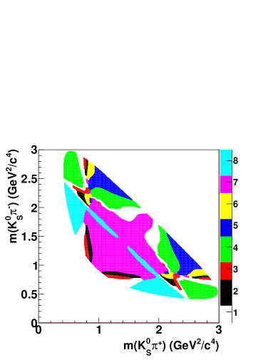
Figure 1: Optimal binning of $D\to K^{0}_{S}\pi^{+}\pi^{-}$ Dalitz plot.

Table 1: Values of the phase terms $c_{i},s_{i}$ for the optimal binning measured by CLEO cleo_2 , and calculated from Belle $D\to K^{0}_{S}\pi^{+}\pi^{-}$ amplitude model. The $\chi^{2}/ndf$ of the agreement between the measured and predicted $c_{i},s_{i}$ is 18.6/16.

	CLEO measurement	Belle model
$c_{1}$	$-0.009\pm 0.088\pm 0.094$	$-0.039$
$c_{2}$	$+0.900\pm 0.106\pm 0.082$	$+0.771$
$c_{3}$	$+0.292\pm 0.168\pm 0.139$	$+0.242$
$c_{4}$	$-0.890\pm 0.041\pm 0.044$	$-0.867$
$c_{5}$	$-0.208\pm 0.085\pm 0.080$	$-0.246$
$c_{6}$	$+0.258\pm 0.155\pm 0.108$	$+0.023$
$c_{7}$	$+0.869\pm 0.034\pm 0.033$	$+0.851$
$c_{8}$	$+0.798\pm 0.070\pm 0.047$	$+0.662$
$s_{1}$	$-0.438\pm 0.184\pm 0.045$	$-0.706$
$s_{2}$	$-0.490\pm 0.295\pm 0.261$	$+0.124$
$s_{3}$	$-1.243\pm 0.341\pm 0.123$	$-0.687$
$s_{4}$	$-0.119\pm 0.141\pm 0.038$	$-0.108$
$s_{5}$	$+0.853\pm 0.123\pm 0.035$	$+0.851$
$s_{6}$	$+0.984\pm 0.357\pm 0.165$	$+0.930$
$s_{7}$	$-0.041\pm 0.132\pm 0.034$	$+0.169$
$s_{8}$	$-0.107\pm 0.240\pm 0.080$	$-0.596$

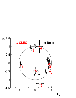
Figure 2: Comparison of phase terms $c_{i},s_{i}$ for the optimal binning measured by CLEO, and calculated from the Belle $D\to K^{0}_{S}\pi^{+}\pi^{-}$ amplitude model.

IV Analysis procedure

The key equation of the analysis (6) holds in the ideal situation with no background, constant efficiency (independent of Dalitz plot variables), and no cross-feed between the bins due to momentum resolution and radiative corrections. In this section, we outline the procedure of the analysis taking the above mentioned effects into account.

IV.1 Efficiency profile

The effect of non-uniform efficiency over the Dalitz plot is canceled out by using the flavor-tagged $D$ sample with the same kinematic properties as the sample for the signal $B$ decay. This approach allows of removal of the systematic error associated with the possible inaccuracy in the description of the detector acceptance in the Monte-Carlo (MC) simulation.

We note that the Equations (2) and (8) do not change after the transformation $p\to\epsilon p$, if the efficiency profile $\epsilon(m^{2}_{+},m^{2}_{-})$ is symmetric: $\epsilon(m^{2}_{+},m^{2}_{-})=\epsilon(m^{2}_{-},m^{2}_{+})$. It means that if the efficiency profile is the same in all three measurements involved (flavor $D$, correlated $\psi(3770)\to D\overline{D}$, and $D$ from $B\to DK$), the resulting measurement will be unbiased even if no efficiency correction is applied.

We match the Dalitz plot efficiency profiles for the flavor $D$ to the one from $B\to DK$ by taking the flavor-tagged $D$ mesons with the same average momentum as the $D$ mesons from $B\to DK$. The center-of-mass (CM) $D$ momentum distribution for $B\to DK$ decays is practically uniform in the narrow range $2.1\mbox{ GeV}/c<p_{D}<2.45\mbox{ GeV}/c$. We assume that the efficiency profile depends mostly on the $D$ momentum and take the flavor-tagged sample with the average momentum of $p_{D}=2.3$ GeV/$c$ (we use a wider range of $D$ momenta than in $B\to DK$ to increase the statistics). The assumption that the efficiency profile depends only on the $D$ momentum is tested using MC simulation, and the remaining difference is treated as the systematic uncertainty.

While calculating $c_{i},s_{i}$, CLEO applies an efficiency correction, therefore the values reported in their analysis correspond to flat efficiency profile. To use the $c_{i},s_{i}$ values in the $\phi_{3}$ analysis, they have to be corrected for the Belle efficiency profile. This correction cannot be performed in a completely model-independent way, since the correction terms include the phase variation inside the bin. Fortunately, the calculations using the Belle $D\to K^{0}_{S}\pi^{+}\pi^{-}$ model show that this correction is negligible even for very large non-uniformity of the efficiency profile. The difference between the uncorrected $c_{i},s_{i}$ terms and those corrected for the efficiency, calculated using the efficiency profile parametrization used in the 605 fb^-1 analysis belle_phi3_3 , does not exceed 0.01, i. e. it is negligible compared to the statistical error.

IV.2 Momentum resolution

Finite momentum resolution leads to migration of events between the bins. In the binned approach, this effect can be corrected for in a non-parametric way. The migration can be described by the linear transformation of the number of events in bins:

$$N^{\prime}_{i}=\sum\alpha_{ik}N_{k},$$ (10)

where $N_{k}$ is the number of events the bin $k$ would contain without the cross-feed, and $N^{\prime}_{i}$ is the reconstructed number of events in the bin $i$. The cross-feed matrix $\alpha_{ik}$ is nearly unit: $\alpha_{ik}\ll 1$ for $i\neq k$. It is obtained from the signal MC simulation with the amplitude measured in Belle’s 605 fb^-1 analysis belle_phi3_3 . In the case of $D\to K^{0}_{S}\pi^{+}\pi^{-}$ decay from $B$, the cross-feed depends on the parameters $x,y$. We assume that this effect is small and neglect it.

Migration of events between the bins occurs also due to final state radiation (FSR). The $c_{i},s_{i}$ terms in the CLEO measurement are not corrected to FSR; we therefore do not simulate FSR to obtain the cross-feed matrix to minimize the bias due to this effect. Comparison of the cross-feed with and without FSR shows that this effect is negligible.

IV.3 Fit procedure

The background contribution has to be accounted for in the calculation of the values $N_{i}$ and $K_{i}$. Statistically the most effective way of calculating the number of signal events (especially in the case of $N_{i}$, where the statistics is a limiting factor) is to perform the unbinned fit in the event selection variables for the events in each bin “$i$” of the Dalitz plot.

Two different approaches are used in this analysis. In the first one, we fit the data distribution in each bin separately, with the number of events for signal and backgrounds as free parameters. Once the numbers of events in bins $N_{i}$ are found, we use them in Eq. 6 to obtain the parameters $x_{\pm},y_{\pm}$. Technically it is done by minimizing the negative logarithmic likelihood of the form

$$-2\log\mathcal{L}(x,y)=-2\sum_{i}\log p(\langle N_{i}\rangle(x,y),N_{i},\sigma_{N_{i}}),$$ (11)

where $\langle N_{i}\rangle(x,y)$ is the expected number of events in the bin $i$ obtained from Eq. 6, $N_{i}$ and $\sigma_{N_{i}}$ are the observed number of events and its error obtained from the data fit. If the probability density function (PDF) $p$ is Gaussian, this procedure translates to the $\chi^{2}$ fit.

The procedure described above does not make any assumptions on the Dalitz distribution of the background events, since the fits in each bin are independent. Thus there is no associated systematic uncertainty. However, in the case of low number of events and many background components this can be a limiting factor. Another solution is to use the combined fit with a common likelihood for all bins. Relative numbers of background events in bins in such a fit can be constrained externally from e. g. MC sample. In addition, in the case of the combined fit, the two-step procedure of first extracting the numbers of signal events, and then using them to obtain $(x,y)$ is not needed — the expected numbers of events $\langle N_{i}\rangle$ as functions of $(x,y)$ can be plugged directly into the likelihood. Thus the variables $(x,y)$ become free parameters of the combined likelihood fit, and the assumption of the Gaussian distribution of the number of signal events is not needed.

Both approaches (separate fits in bins, and the combined fit) are tested with the control sample and the MC simulation. We choose the combined fit approach as the baseline, but the approach with separate fits in bins is also used: it allows to clearly demonstrate the $CP$ asymmetry of the number of events in bins.

V Event selection

We use a data sample of $772\times 10^{6}$ $B\overline{B}$ pairs collected by the Belle detector. The decay chains $B^{+}\to DK^{+}$ and $B^{\pm}\to D\pi^{\pm}$  are selected for the analysis. The neutral $D$ meson is reconstructed in the $K^{0}_{S}\pi^{+}\pi^{-}$ final state in all cases. We also select decays of $D^{*+}\to D^{0}\pi^{+}$ produced via the $e^{+}e^{-}\to c\bar{c}$ continuum process as a high-statistics sample to determine the terms related to flavor-tagged $D^{0}\to K^{0}_{S}\pi^{+}\pi^{-}$ decay.

The Belle detector is described in detail elsewhere belle ; svd2 . It is a large-solid-angle magnetic spectrometer consisting of a silicon vertex detector (SVD), a 50-layer central drift chamber (CDC) for charged particle tracking and specific ionization measurement ($dE/dx$), an array of aerogel threshold Cherenkov counters (ACC), time-of-flight scintillation counters (TOF), and an array of CsI(Tl) crystals for electromagnetic calorimetry (ECL) located inside a superconducting solenoid coil that provides a 1.5 T magnetic field. An iron flux return located outside the coil is instrumented to detect $K_{L}$ mesons and identify muons (KLM).

Charged tracks are required to satisfy criteria based on the quality of the track fit and the distance from the interaction point (IP). We require each track to have a transverse momentum greater than 100 MeV/$c$, and the impact parameter relative to the IP of the beams less than 2 mm in the transverse and less than 10 mm in longitudinal projections. Separation of kaons and pions is accomplished by combining the responses of the ACC and the TOF with the $dE/dx$ measurement from the CDC. Neutral kaons are reconstructed from pairs of oppositely charged tracks with an invariant mass $M_{\pi\pi}$ within $7$ MeV/$c^{2}$ of the nominal $K^{0}_{S}$ mass, flight distance from the IP in the plane transverse to the beam axis grater than 0.1 mm, and the cosine of the angle between the projections of flight direction and its momentum greater than 0.95.

To determine the terms for flavor-tagged $D^{0}\to K^{0}_{S}\pi^{+}\pi^{-}$ decay we use $D^{*\pm}$ mesons produced via the $e^{+}e^{-}\to c\bar{c}$ continuum process. The flavor of the neutral $D$ meson is tagged by the charge of the slow pion in the decay $D^{*+}\to D^{0}\pi^{+}$. The slow pion track is required to originate from the $D^{0}$ decay vertex to improve the momentum and angular resolution. The selection of signal candidates is based on two variables, the invariant mass of the neutral $D$ candidates $M_{D}=M_{K^{0}_{S}\pi^{+}\pi^{-}}$ and the difference of the invariant masses of the $D^{*\pm}$ and the neutral $D$ candidates $\Delta M=M_{(K^{0}_{S}\pi^{+}\pi^{-})_{D}\pi}-M_{K^{0}_{S}\pi^{+}\pi^{-}}$. We retain the events satisfying the following criteria: $1800\mbox{ MeV}/c^{2}<M_{D}<1920$ MeV/$c^{2}$ and $\Delta M<0.15$ MeV/$c^{2}$. We also require the momentum of the $D^{0}$ candidate in the CM frame $p_{D}$ to be greater than 1.5 GeV/$c$. About 15% of selected events contain more than one $D^{*\pm}$ candidate that satisfies the requirements above; in that case we keep only one randomly selected candidate.

Selection of $B^{\pm}\to DK^{\pm}$ and $B^{\pm}\to D\pi^{\pm}$ samples is based on the CM energy difference $\Delta E=\sum E_{i}-E_{\rm beam}$ and the beam-constrained $B$ meson mass $M_{\rm bc}=\sqrt{E_{\rm beam}^{2}-(\sum\vec{p}_{i})^{2}}$, where $E_{\rm beam}$ is the CM beam energy, and $E_{i}$ and $\vec{p}_{i}$ are the CM energies and momenta of the $B$ candidate decay products. We select events with $M_{\rm bc}>5.2$ GeV/$c^{2}$ and $|\Delta E|<0.18$ GeV for further analysis. We also impose a requirement on the invariant mass of the neutral $D$ candidate $|M_{K^{0}_{S}\pi^{+}\pi^{-}}-M_{D^{0}}|<11$ MeV/$c^{2}$.

Further separation of the background from $e^{+}e^{-}\to q\bar{q}$ ($q=u,d,s,c$) continuum events is done by calculating two variables that characterize the event shape. One is the cosine of the thrust angle $\cos\theta_{\rm thr}$, where $\theta_{\rm thr}$ is the angle between the thrust axis of the $B$ candidate daughters and that of the rest of the event, calculated in the CM frame. The other is a Fisher discriminant $\mathcal{F}$ composed of 11 parameters fisher : the production angle of the $B$ candidate, the angle of the $B$ thrust axis relative to the beam axis, and nine parameters representing the momentum flow in the event relative to the $B$ thrust axis in the CM frame.

In both flavor $D^{0}$ and $B^{\pm}\to DK^{\pm}$ ($B^{\pm}\to D\pi^{\pm}$) samples the momenta of the tracks forming a $D^{0}$ candidate are fitted to the nominal $D^{0}$ mass in the calculation of the Dalitz plot variables.

VI Flavor-tagged sample $D^{*+}\to D^{0}\pi^{+}$, $D\to K^{0}_{S}\pi^{+}\pi^{-}$

The numbers of events $K_{i}$ in bins of the flavor-tagged $D\to K^{0}_{S}\pi^{+}\pi^{-}$ decay are obtained from the two-dimensional unbinned fit of the distribution of variables $M_{D}$ and $\Delta M$. The fits in each Dalitz plot bin are done independently. We take the candidates in the CM $D$ momentum range $1.8\mbox{ GeV}/c<p_{D}<2.8\mbox{ GeV}/c$. It provides the same average $p_{D}$ as in $B\to DK$ decays ($p_{D}=2.3$ GeV/$c$) to reduce the influence of the efficiency profile on $\phi_{3}$ measurement (see Section IV.1).

The fit uses the signal PDF and two background components: purely random combinatorial background and the background with real $D^{0}$ and random slow pion track. The signal distribution is a product of the PDF’s for $M_{D}$ (triple Gaussian) and $\Delta M$ (sum of bifurcated Student distribution and bifurcated Gaussian distribution). The combinatorial background is parametrized by the linear function in $M_{D}$ and by the function with a kinematic threshold at the $\pi^{+}$ mass in $\Delta M$. The random slow pion background is parametrized as a product of signal $M_{D}$ distribution and the combinatorial $\Delta M$ background shape.

The parameters of the signal and background distributions are obtained from the data fit. The parameters of the signal PDF are constrained to be the same in all bins. The free parameters in each bin are the number of signal events $K_{i}$, the parameters of the background distribution and fractions of the background components.

The fit results of the flavor sample for the whole Dalitz plot are shown in Fig. 3. The number of signal events calculated from the integral of the signal distribution is $426938\pm 825$, the background fraction in the signal box $|M_{D}-m_{D^{0}}|<11$ MeV/$c^{2}$, $144.5\mbox{ MeV}/c^{2}<\Delta M<146.5$ MeV/$c^{2}$ is $10.1\pm 0.1$%. The numbers of events in bins are shown in Table 2.

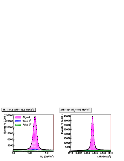
Figure 3: Projections of the flavor-tagged $D^{*+}\to D^{0}\pi^{+}$, $D\to K^{0}_{S}\pi^{+}\pi^{-}$ data with $1.8\mbox{ GeV}/c<p_{D}<2.8\mbox{ GeV}/c$ onto (a) $M_{D}$ and (b) $\Delta M$ variables. Histograms show fitted signal and background contributions, points with the error bars are the data. Full $D\to K^{0}_{S}\pi^{+}\pi^{-}$ Dalitz plot is used.

Table 2: Numbers of events in Dalitz plot bins for the flavor-tagged $D^{*+}\to D^{0}\pi^{+}$, $D\to K^{0}_{S}\pi^{+}\pi^{-}$ sample with $1.8\mbox{ GeV}/c<p_{D}<2.8\mbox{ GeV}/c$. Results of the 2D $(\Delta M,M_{D})$ fit to data.

Bin $i$	$K_{i}(p_{D}\in(1.8,2.8))$
-8	$26450\pm 181$
-7	$22476\pm 196$
-6	$1765\pm 68$
-5	$13146\pm 143$
-4	$26482\pm 202$
-3	$1601\pm 58$
-2	$1827\pm 63$
-1	$0$$8770\pm 124$
1	$43261\pm 255$
2	$58005\pm 268$
3	$62808\pm 274$
4	$44513\pm 253$
5	$21886\pm 177$
6	$28876\pm 197$
7	$48001\pm 265$
8	$0$$9279\pm 125$
Total	$426938\pm 825$$0$

VII Selection of $B^{\pm}\to D\pi^{\pm}$ and $B^{\pm}\to DK^{\pm}$ samples

The decays $B^{\pm}\to DK^{\pm}$ and $B^{\pm}\to D\pi^{\pm}$ have similar topology and background sources and their selection is performed in a similar way. The mode $B^{\pm}\to D\pi^{\pm}$ has an order of magnitude larger branching ratio and small amplitude ratio $r_{B}\sim 0.01$ due to small ratio of the weak coefficients $|V_{ub}^{\vphantom{*}}V^{*}_{cd}|/|V_{cb}^{\vphantom{*}}V^{*}_{ud}|\sim 0.02$ and additional color suppression factor as in the case of $B^{\pm}\to DK^{\pm}$. This mode is used as a control sample to test the procedures of the background extraction and Dalitz plot fit. Also, the resolution scale factors and Dalitz plot structure of some background components are constrained from the control sample and used in the signal fit.

Extraction of the number of signal events is performed by fitting the 4D distribution of variables $M_{\rm bc}$, $\Delta E$, $\cos\theta_{\rm thr}$ and $\mathcal{F}$. The fit to $B^{\pm}\to D\pi^{\pm}$ sample uses three background components in addition to the signal PDF. These are:

• Combinatorial background from $e^{+}e^{-}\to q\overline{q}$ process, where $q=(u,d,s,c)$.

• Random $B\overline{B}$ background, where the tracks forming the $B^{\pm}\to D\pi^{\pm}$ candidate come from decays of both $B$ mesons in the event. The number of possible $B$ decay combinations that contribute to this background is large, therefore both the Dalitz distribution and $(M_{\rm bc},\Delta E)$ distribution are quite smooth.

• Peaking $B\overline{B}$ background, where all tracks forming the $B^{\pm}\to D\pi^{\pm}$ candidate come from the same $B$ meson. This kind of background is dominated by the $B\to D^{*}\pi$ decays with lost $\pi$ or $\gamma$ from $D^{*}$ decay.

The $B^{\pm}\to DK^{\pm}$ fit includes in addition the background from $B^{\pm}\to D\pi^{\pm}$ decays with pion misidentified as kaon.

The PDF for the signal parametrization (as well as for each of the background components) is a product of $(M_{\rm bc},\Delta E)$ and $(\cos\theta_{\rm thr},\mathcal{F})$ PDFs. The $(M_{\rm bc},\Delta E)$ PDF is a sum of two 2D Gaussian distributions (core and wide) with the correlation between $M_{\rm bc}$ and $\Delta E$. We use common parametrization for the $\cos\theta_{\rm thr},\mathcal{F}$ distribution for signal and all background components. The distribution is parametrized by the sum of two functions (with different coefficients) of the form

$$\begin{split}p(x,\mathcal{F})=&\exp(C_{1}x+C_{2}x^{2}+C_{3}x^{3})\times\\ &G(\mathcal{F},F_{0}(x),\sigma_{FL}(x),\sigma_{FR}(x)),\end{split}$$ (12)

where $x=\cos\theta_{\rm thr}$, $G(x,F,\sigma_{R},\sigma_{R})$ is the bifurcated Gaussian distribution with the mean $F$ and the widths $\sigma_{L}$ and $\sigma_{R}$, and functions $F_{0}$, $\sigma_{FL}$ and $\sigma_{FR}$ are the polynomials which contain only even powers of $x$.

Combinatorial background from continuum $e^{+}e^{-}\to q\overline{q}$ production is obtained from the experimental sample collected at the CM energy below $\Upsilon(4S)$ resonance (off-resonance data). The parametrization in variables $(\cos\theta_{\rm thr},\mathcal{F})$ is the same as described for the signal PDF. The parametrization in $(M_{\rm bc},\Delta E)$ is the product of exponential distribution in $\Delta E$ and the empirical shape proposed by the Argus collaboration argus in $M_{\rm bc}$:

$$p_{\rm comb}(M_{\rm bc},\Delta E)=\exp(-\alpha\Delta E)M_{\rm bc}\sqrt{y}\exp(-cy),$$ (13)

where $y=1-M_{\rm bc}/E_{\rm beam}$, and $E_{\rm beam}$ is the CM beam energy.

Random $B\overline{B}$ background is obtained from generic MC sample. Generator information is used to select only the events where the candidate is formed from tracks coming from both $B$ mesons. The $(M_{\rm bc},\Delta E)$ distribution of this background is parametrized by the sum of three components:

• product of exponential (in $\Delta E$) and Argus (in $M_{\rm bc}$) functions, as for continuum background,

• product of exponential in $\Delta E$ and bifurcated Gaussian distribution in $M_{\rm bc}$, where the mean of the Gaussian distribution is linear as a function of $\Delta E$.

• two-dimensional Gaussian distribution in $\Delta E,M_{\rm bc}$ with correlation (asymmetric in $M_{\rm bc}$).

Peaking $B\overline{B}$ backgrounds are parametrized by the same function as the random $B\overline{B}$ background. The background coming from $B^{+}B^{-}$ and $B^{0}\overline{B}{}^{0}$ decays is treated separately in $(M_{\rm bc},\Delta E)$ variables, while the common $(\cos\theta_{\rm thr},\mathcal{F})$ distribution is used. In the case of $B^{\pm}\to DK^{\pm}$ fit, we take the $B^{\pm}\to D\pi^{\pm}$ events with pion misidentified as kaon as a separate background category. The distributions of $M_{\rm bc},\Delta E$ and $\cos\theta_{\rm thr},\mathcal{F}$ variables are parametrized in the same way as for the signal events and are obtained from MC simulation.

The Dalitz plot distributions of the background components are discussed in the next section. Note that the Dalitz distribution is described by the relative number of events in bins. The numbers of events in bins can be taken as free parameters in the fit, thus there will be no uncertainty due to Dalitz plot description of the background in such an approach. This procedure is justified for the background that is well separated from the signal (such as peaking $B\overline{B}$ background in the case of $B^{\pm}\to D\pi^{\pm}$), or if the background is constrained by much larger number of events than the signal (such as the continuum background).

The results of the fit to $B^{\pm}\to D\pi^{\pm}$ and $B^{\pm}\to DK^{\pm}$ data with the full Dalitz plot taken are shown in Figs 4 and 5, respectively. We obtain a total of $19106\pm 147$ signal $B^{\pm}\to D\pi^{\pm}$ events and $1176\pm 43$ signal $B^{\pm}\to DK^{\pm}$ events — 55% more than in the 605 fb^-1 model-dependent analysis belle_phi3_3 . The improvement partially comes from larger integrated luminosity, and partially from the better selection efficiency due to improved tracking procedures.

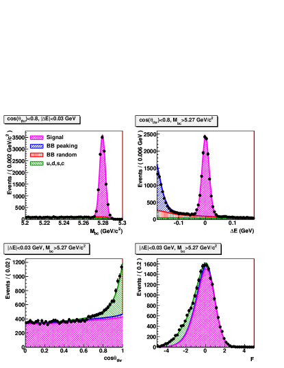
Figure 4: Projections of the $B^{\pm}\to D\pi^{\pm}$ data onto (a) $M_{\rm bc}$, (b) $\Delta E$, (c) $\cos\theta_{\rm thr}$ and (d) $\mathcal{F}$ variables. Histograms show fitted signal and background contributions, points with the error bars are the data. Full $D\to K^{0}_{S}\pi^{+}\pi^{-}$ Dalitz plot is used.

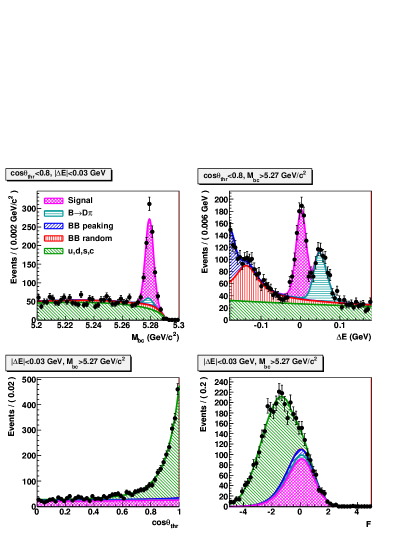
Figure 5: Projections of the $B^{\pm}\to DK^{\pm}$ data onto (a) $M_{\rm bc}$, (b) $\Delta E$, (c) $\cos\theta_{\rm thr}$ and (d) $\mathcal{F}$ variables. Histograms show fitted signal and background contributions, points with the error bars are the data. Full $D\to K^{0}_{S}\pi^{+}\pi^{-}$ Dalitz plot is used.

VIII Data fits in bins

The data fits in bins for both $B^{\pm}\to D\pi^{\pm}$ and $B^{\pm}\to DK^{\pm}$ are performed with two different procedures: separate fits for the number of events in bins, and the combined fit with the free parameters $(x,y)$, as discussed in Section IV.3. The combined fit is used to obtain the final values for $(x,y)$, while the separate fits provide the cross-check of the fit procedure and a way to visualize the $CP$-violating effect. The study with MC pseudo-experiments is performed to check that the observed difference in the fit results between the two approaches agrees with the expectation.

In the case of separate fits in bins, we first perform the fit to all events in the Dalitz plot. The fit uses background shapes fixed from the generic MC simulation of continuum and $B\overline{B}$ decays. The signal shape is fixed from the signal MC sample except that we float the mean values of $\Delta E$ and $M_{\rm bc}$ and width scale factors. As a next step, we fit the 4D $(M_{\rm bc},\Delta E,\cos\theta_{\rm thr},\mathcal{F})$ distributions in each bin separately. The free parameters of each fit are the number of signal events, and the number of events in each background category.

The numbers of signal events in bins extracted from the fits are given in Table 3. These numbers are used in the fit to extract $(x,y)$ using (6) after the cross-feed and efficiency correction for both $N_{i}$ and $K_{i}$. Figure 6 illustrates the results of this fit. The numbers of signal events in bins separately for $B^{+}$ and $B^{-}$ are shown in Fig. 6(a) together with the numbers of events in the flavor sample (appropriately scaled). The difference in the number of signal events shown in Fig. 6(b) does not reveal $CP$ violation. Figures 6(c) and (d) show the difference of the numbers of signal events for $B^{+}$ ($B^{-}$) data and scaled flavor sample, both for the data and after the $(x,y)$ fit. The $\chi^{2}/ndf$ is reasonable for both the $(x,y)$ fit and for the agreement with the purely flavor-specific amplitude.

Unlike $B^{\pm}\to D\pi^{\pm}$, the $B^{\pm}\to DK^{\pm}$ sample shows significantly different numbers of events in bins of $B^{+}$ and $B^{-}$ data (see Fig. 7(b) and Table 4). The probability to obtain this difference as a result of statistical fluctuation is 0.42%. This number can be taken as the model-independent measure of the $CP$ violation significance. The significance of $\phi_{3}$ being nonzero is in general smaller since $\phi_{3}\neq 0$ results in a specific pattern of charge asymmetry. The fit of the numbers of events to the expected pattern described by the parameters $(x,y)$ shows a good quality 7(c,d), i. e. is consistent with the hypothesis that the observed $CP$ violation is solely explained by the mechanism involving nonzero $\phi_{3}$.

Table 3: Numbers of events in Dalitz plot bins for the $B^{\pm}\to D\pi^{\pm}$, $D\to K^{0}_{S}\pi^{+}\pi^{-}$ sample with the optimal binning. Results of the independent 4D fits with variables $(M_{\rm bc},\Delta E,\cos\theta_{\rm thr},\mathcal{F})$ fit to data.

Bin $i$	$N^{-}_{i}$	$N^{+}_{i}$
-8	$564.2\pm 25.3$	$587.0\pm 25.7$
-7	$462.3\pm 23.8$	$462.8\pm 23.9$
-6	$47.9\pm 7.7$	$39.2\pm 7.2$
-5	$314.1\pm 19.0$	$286.2\pm 18.2$
-4	$592.6\pm 26.5$	$645.7\pm 27.8$
-3	$22.2\pm 6.2$	$27.2\pm 6.3$
-2	$42.7\pm 7.6$	$54.0\pm 8.7$
-1	$190.8\pm 15.4$	$210.8\pm 16.3$
1	$959.2\pm 32.6$	$980.2\pm 33.1$
2	$1288.7\pm 37.0$$0$	$1295.9\pm 37.1$$0$
3	$1395.8\pm 38.4$$0$	$1352.2\pm 37.9$$0$
4	$1045.5\pm 34.7$$0$	$1065.1\pm 34.9$$0$
5	$479.3\pm 23.3$	$532.2\pm 24.5$
6	$623.7\pm 26.0$	$663.5\pm 26.7$
7	$1081.0\pm 35.3$$0$	$1049.2\pm 34.8$$0$
8	$210.0\pm 16.1$	$212.1\pm 16.3$
Total	$9467.1\pm 103.6$	$9639.1\pm 104.7$

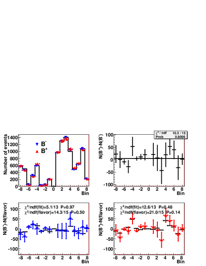
Figure 6: Results of the fit of $B^{\pm}\to D\pi^{\pm}$ control sample. (a) Numbers of events in bins of $D\to K^{0}_{S}\pi^{+}\pi^{-}$ Dalitz plot: from $B^{-}\to D\pi^{-}$ (red), $B^{+}\to D\pi^{+}$ (blue) and flavor sample (histogram). (b) Difference of the number of events from $B^{+}\to D\pi^{+}$ and $B^{-}\to D\pi^{-}$ decays. (c) Difference of the number of events from $B^{-}\to D\pi^{-}$ and flavor sample (normalized to the total number of $B^{-}\to D\pi^{-}$ decays): data (points with the error bars), and as a result of the $(x,y)$ fit (horizontal bars). (d) Same for $B^{+}\to D\pi^{+}$ data.

Table 4: Numbers of events in Dalitz plot bins for the $B^{\pm}\to DK^{\pm}$, $D\to K^{0}_{S}\pi^{+}\pi^{-}$ sample with the optimal binning. Results of the independent 4D fits with variables $(M_{\rm bc},\Delta E,\cos\theta_{\rm thr},\mathcal{F})$ fit to data.

Bin $i$	$N^{-}_{i}$	$N^{+}_{i}$
-8	$49.8\pm 8.2$	$37.8\pm 7.5$
-7	$42.2\pm 8.6$	$24.9\pm 7.2$
-6	$0$$0.0\pm 1.9$	$0$$3.4\pm 2.9$
-5	$0$$9.6\pm 4.5$	$23.6\pm 6.2$
-4	$32.9\pm 7.5$	$42.1\pm 8.3$
-3	$0$$3.5\pm 2.8$	$0$$0.7\pm 2.5$
-2	$11.3\pm 4.1$	$0$$0.0\pm 1.3$
-1	$16.6\pm 5.4$	$0$$7.7\pm 4.4$
1	$37.6\pm 8.0$	$65.1\pm 9.9$
2	$68.6\pm 9.6$	$75.5\pm 9.8$
3	$0$$83.4\pm 10.1$	$0$$82.4\pm 10.2$
4	$49.3\pm 9.1$	$0$$86.5\pm 11.4$
5	$34.0\pm 7.3$	$38.3\pm 7.6$
6	$34.8\pm 6.8$	$41.9\pm 7.5$
7	$0$$70.8\pm 10.6$	$46.4\pm 9.0$
8	$0$$9.4\pm 4.3$	$14.2\pm 5.1$
Total	$574.9\pm 29.9$	$601.6\pm 30.8$

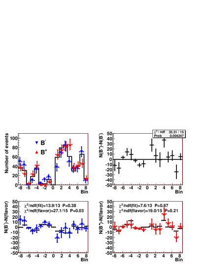
Figure 7: Results of the fit of $B^{\pm}\to DK^{\pm}$ control sample. (a) Numbers of events in bins of $D\to K^{0}_{S}\pi^{+}\pi^{-}$ Dalitz plot: from $B^{-}\to DK^{-}$ (red), $B^{+}\to DK^{+}$ (blue) and flavor sample (histogram). (b) Difference of the number of events from $B^{+}\to DK^{+}$ and $B^{-}\to DK^{-}$ decays. (c) Difference of the number of events from $B^{-}\to DK^{-}$ and flavor sample (normalized to the total number of $B^{-}\to DK^{-}$ decays): data (points with the error bars), and as a result of the $(x,y)$ fit (horizontal bars). (d) Same for $B^{+}\to DK^{+}$ data.

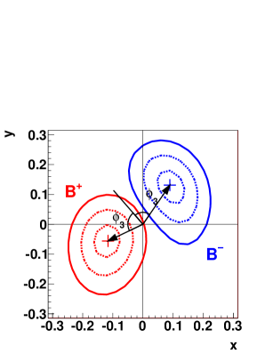
Figure 8: One-, two-, and three standard deviations levels for $x,y$ fit of $B^{\pm}\to DK^{\pm}$ mode.

The default combined fit uses the constraint of the random $B\overline{B}$ background in bins from the generic MC, and $x_{\pm},y_{\pm}$ variables as free parameters. Fits to $B^{+}$ and $B^{-}$ data are performed separately. Additional free parameters are the numbers of continuum and peaking $B\overline{B}$ backgrounds in each bin, fraction of the random $B\overline{B}$ background, and means and scale factors of the signal $M_{\rm bc}$ and $\Delta E$ distributions. The values of $x,y$ are then corrected for the fit bias obtained from MC pseudo-experiments. The value of the bias depends on the initial $x$ and $y$ values and is of the order $5\times 10^{-3}$ for $B^{\pm}\to DK^{\pm}$ sample and less than $10^{-3}$ for $B^{\pm}\to D\pi^{\pm}$ sample.

The values of $x,y$ parameters and their statistical correlations obtained from the combined fit are as follows:

$$\begin{split}x_{-}&=-0.0045\pm 0.0087\pm 0.0050\pm 0.0026,\\ y_{-}&=-0.0231\pm 0.0107\pm 0.0050\pm 0.0065,\\ \rm{corr}(x_{-},y_{-})&=-0.189,\\ x_{+}&=-0.0172\pm 0.0089\pm 0.0060\pm 0.0026,\\ y_{+}&=+0.0129\pm 0.0103\pm 0.0060\pm 0.0065,\\ \rm{corr}(x_{+},y_{+})&=-0.205\end{split}$$ (14)

for $B^{\pm}\to D\pi^{\pm}$ control sample and

$$\begin{split}x_{-}&=+0.095\pm 0.045\pm 0.014\pm 0.017,\\ y_{-}&=+0.137^{+0.053}_{-0.057}\pm 0.019\pm 0.029,\\ \rm{corr}(x_{-},y_{-})&=-0.315,\\ x_{+}&=-0.110\pm 0.043\pm 0.014\pm 0.016,\\ y_{+}&=-0.050^{+0.052}_{-0.055}\pm 0.011\pm 0.021,\\ \rm{corr}(x_{+},y_{+})&=+0.059\end{split}$$ (15)

for $B^{\pm}\to DK^{\pm}$ sample. Here the first error is statistical, the second error is the systematic uncertainty, and the third error is the uncertainty due to the errors of $c_{i},s_{i}$ terms. The measured values of $(x_{\pm},y_{\pm})$ with their likelihood contours are shown in Fig. 8.

IX Systematic errors

Systematic errors in the $x,y$ fit are obtained for the default procedure of the combined fit with the optimal binning. The systematic errors are summarized in Table 5.

The uncertainty of the signal shape used in the fit includes the following sources:

• Choice of parametrization used to model the shape. The corresponding uncertainty is estimated by using the non-parametric (Keys) function instead of parametrized distribution.

• Possible correlation between the $(M_{\rm bc},\Delta E)$ and $(\cos\theta_{\rm thr},\mathcal{F})$ distributions. To estimate its effect we use 4D binned histogram to describe the distribution.

• MC description of the ($\cos\theta_{\rm thr}$, $\mathcal{F}$) distribution. Its effect is estimated by floating the parameters of the distribution in the fit to $B^{\pm}\to D\pi^{\pm}$ control sample.

• Dependence of the signal width on the Dalitz plot bin. The uncertainty due to this effect is estimated by performing the $B^{\pm}\to D\pi^{\pm}$ fit with the shape parameters floated separately for each bin, and then using the results in the fit to $B^{\pm}\to DK^{\pm}$ data.

We do not assign the uncertainty due to the difference in $(M_{\rm bc},\Delta E)$ shape between the MC and data since the width of the signal distribution is calibrated on $B^{\pm}\to D\pi^{\pm}$ data.

In the uncertainty of the continuum background shape, the same four sources are considered as for the signal distribution. The uncertainty due to the choice of parametrization is estimated similarly by using the Keys function. The effect of possible correlation between the $(M_{\rm bc},\Delta E)$ and $(\cos\theta_{\rm thr},\mathcal{F})$ distributions is estimated by using the distribution split into the sum of two components ($u,d,s$ and charm contributions) with independent $(M_{\rm bc},\Delta E)$ and $(\cos\theta_{\rm thr},\mathcal{F})$ shapes. The uncertainty due to MC description of the $(M_{\rm bc},\Delta E)$ and $(\cos\theta_{\rm thr},\mathcal{F})$ distributions is estimated by floating their parameters in the $B^{\pm}\to D\pi^{\pm}$ fit. To estimate the effect of possible correlation of the shape with the Dalitz plot variables we fit the shapes separately in each Dalitz plot bin.

The uncertainties of the shapes of random and peaking $B\overline{B}$ backgrounds are estimated conservatively by performing the fit with $\Delta E>-0.1$ GeV — this requirement rejects the peaking $B\overline{B}$ background and a large part of the random $B\overline{B}$ background.

In the case of the fit of $B^{\pm}\to DK^{\pm}$ sample, the uncertainty of the $B^{\pm}\to D\pi^{\pm}$ background shape in $(\cos\theta_{\rm thr},\mathcal{F})$ variables is estimated by taking the $(\cos\theta_{\rm thr},\mathcal{F})$ shape for signal events. The Dalitz plot uncertainty is estimated by using the number of flavor-tagged events in bins (rather than the number of $B^{\pm}\to D\pi^{\pm}$ events used in the default fit). Uncertainties due to possible correlations are treated as in the case of the signal distribution.

The uncertainty due to Dalitz plot efficiency shape appears because of a difference in average efficiency for the flavor and $B^{\pm}\to DK^{\pm}$ samples. The maximum difference of 1.5% is obtained in the MC study. The uncertainty is obtained from the maximum of two quantities:

• RMS of $x$ and $y$ from smearing the numbers of events in the flavor sample $K_{i}$ by 1.5%.

• Bias of $x$ and $y$ between the fits with and without efficiency correction for $K_{i}$ obtained from signal MC.

The uncertainty due to cross-feed of events between bins is conservatively estimated by taking the bias between the fits with and without cross-feed.

The uncertainty arising from the finite sample of flavor-tagged $D\to K^{0}_{S}\pi^{+}\pi^{-}$ decays is evaluated by varying the numbers of flavor-tagged events in bins $K_{i}$ within their statistical errors.

The final results for $x,y$ are corrected for the fit bias obtained from the fits of MC pseudo-experiments. The uncertainty due to the fit bias is taken from the difference of biases for various input values of $x$ and $y$.

The uncertainty due to errors of $c_{i}$ and $s_{i}$ parameters is obtained by smearing the $c_{i}$ and $s_{i}$ values within their total errors and repeating the fits for the same experimental data. We have performed a study of this procedure using the MC pseudo-experiments and analytical calculations. We find that the uncertainty obtained this way is sample-dependent for small $B$ data samples and its average scales inversely proportional to the square root of sample size. It reaches a constant value for large $B$ data samples (in the systematics-dominated case). This explains a somewhat higher uncertainty compared to the CLEO estimate given in cleo_2 obtained in the limit of very large $B$ sample. In addition, the uncertainty in $x,y$ is proportional to $r_{B}$, and thus the uncertainty of the phases $\phi_{3}$ and $\delta_{B}$ is independent of $r_{B}$. As a result, the uncertainty of $x,y$ in the $B^{\pm}\to DK^{\pm}$ sample fit is 3–4 times larger than for $B^{\pm}\to D\pi^{\pm}$.

Table 5: Systematic errors of $x,y$ measurement for $B^{\pm}\to D\pi^{\pm}$ and $B^{\pm}\to DK^{\pm}$ samples in units of $10^{-3}$.

	$B^{\pm}\to D\pi^{\pm}$				$B^{\pm}\to DK^{\pm}$
Source of uncertainty	$\Delta x_{-}$	$\Delta y_{-}$	$\Delta x_{+}$	$\Delta y_{+}$	$\Delta x_{-}$	$\Delta y_{-}$	$\Delta x_{+}$	$\Delta y_{+}$
Signal shape	$0.9$	$1.9$	$1.1$	$5.0$	$7.3$	$7.4$	$7.3$	$5.1$
$u,d,s,c$ continuum background	$0.9$	$1.4$	$0.8$	$1.3$	$6.7$	$5.6$	$6.6$	$3.2$
$B\overline{B}$ background	$3.3$	$1.6$	$4.5$	$1.1$	$7.8$	$12.2$	$7.2$	$6.1$
$B^{\pm}\to D\pi^{\pm}$ background	$-$	$-$	$-$	$-$	$1.2$	$4.2$	$1.9$	$1.9$
Dalitz plot efficiency	$3.0$	$1.9$	$3.2$	$1.6$	$4.8$	$2.0$	$5.6$	$2.1$
Cross-feed between bins	$0.4$	$3.0$	$0.7$	$0.9$	$0.4$	$9.0$	$0.6$	$3.0$
Flavor-tagged statistics	$1.7$	$2.0$	$1.6$	$2.0$	$1.5$	$2.7$	$1.7$	$1.9$
Fit bias	$0.4$	$0.5$	$0.4$	$0.5$	$3.2$	$5.8$	$3.2$	$5.8$
$c_{i},s_{i}$ precision	$2.6$	$6.5$	$2.6$	$6.5$	$10.1$	$22.5$	$7.2$	$17.4$
Total without $c_{i}$,$s_{i}$ precision	$5.0$	$5.0$	$6.0$	$6.0$	$14.0$	$19.4$	$14.0$	$11.3$
Total	$5.6$	$8.2$	$6.5$	$8.8$	$17.3$	$29.7$	$15.7$	$20.7$

X Results for $\phi_{3}$, $r_{B}$ and $\delta_{B}$

We use frequentist treatment with the Feldman-Cousins ordering to obtain the physical parameters $\mu=(\phi_{3},r_{B},\delta_{B})$ from the measured parameters $z=(x_{-},y_{-},x_{+},y_{+})$ as was done in the previous Belle analyses. In essence, the confidence level $\alpha$ for a set of physical parameters $\mu$ is calculated as

$$\alpha(\mu)=\int\limits_{\mathcal{D}(\mu)}p(z|\mu)dz\left/\int\limits_{\infty}p(z|\mu)dz\right.,$$ (16)

where $p(z|\mu)$ is the probability density to obtain the measurement result $z$ given the set of physics parameters $\mu$. The integration domain $\mathcal{D}(\mu)$ is given by the likelihood ratio (Feldman-Cousins) ordering:

$$\frac{p(z|\mu)}{p(z|\mu_{\rm best}(z))}>\frac{p(z_{0}|\mu)}{p(z_{0}|\mu_{\rm best}(z_{0}))},$$ (17)

where $\mu_{\rm best}(z)$ is $\mu$ that maximizes $p(z|\mu)$ for the given $z$, and $z_{0}$ is the result of the data fit.

The difference with the previous Belle analyses is that the probability density $p(z|\mu)$ is a multivariate Gaussian PDF with the errors and correlations between $x_{\pm}$ and $y_{\pm}$ taken from the data fit result. In the previous analyses, this PDF was taken from MC pseudo-experiments.

As a result of this procedure, we obtain the confidence levels (CL) for the set of physical parameters $\phi_{3},r_{B},\delta_{B}$. The confidence levels for one and two standard deviations are taken at 20% and 74% (the case of three-dimensional Gaussian distribution). The projections of the 3D surfaces bounding one and two standard deviations volumes onto $\phi_{3}$ variable, and $(\phi_{3},r_{B})$ and $(\phi_{3},\delta_{B})$ planes are shown in Fig. 9.

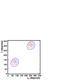
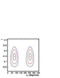
Figure 9: Two-dimensional projections of confidence region onto $(\phi_{3},\delta_{B})$ and $(\phi_{3},r_{B})$ planes (one-, two-, and three standard deviations).

Systematic errors in $\mu$ are obtained by varying the measured parameters $z$ within their systematic errors (Gaussian distribution is taken) and calculating the RMS of $\mu_{\rm best}(z)$. In this calculation we assume that the systematic errors are uncorrelated. In the case of $c_{i},s_{i}$ systematics, we test that assumption: when the fluctuation in $c_{i}$ and $s_{i}$ is generated, we perform the fits to both $B^{+}$ and $B^{-}$ data with the same fluctuated $c_{i},s_{i}$. We observe no significant correlation between resulting $x_{-}$ and $x_{+}$ ($y_{-}$ and $y_{+}$).

The final results are:

$$\begin{split}\phi_{3}&=(77.3^{+15.1}_{-14.9}\pm 4.2\pm 4.3)^{\circ}\\ r_{B}&=0.145\pm 0.030\pm 0.011\pm 0.011\\ \delta_{B}&=(129.9\pm 15.0\pm 3.9\pm 4.7)^{\circ},\end{split}$$ (18)

where the first error is statistical, the second is systematic error without $c_{i},s_{i}$ uncertainty, and the third error is due to $c_{i},s_{i}$ uncertainty.

We do not calculate the statistical significance of $CP$ violation as it is done in the previous analyses by taking the CL for $\phi_{3}=0$: this number is purely based on the behavior of the tails of $p(z|\mu)$ distribution far from the central value, and Gaussian assumption can lead to overestimation of $CP$ violation significance. As a preliminary number we use the estimate of probability of the fluctuation in the difference of number of events in bins for $B^{+}$ and $B^{-}$ data: the probability of such fluctuation in the case of $CP$ conservation is $p=0.42$%.

XI Conclusion

We report the results of a measurement of the unitarity triangle angle $\phi_{3}$ using a model-independent Dalitz plot analysis of $D\to K^{0}_{S}\pi^{+}\pi^{-}$ decay in the process $B^{\pm}\to DK^{\pm}$. The measurement was performed with a full data sample of 711 fb^-1 ($772\times 10^{6}$ $B\overline{B}$ pairs) collected by the Belle detector at $\Upsilon(4S)$. The model independence is reached by binning the Dalitz plot of $D\to K^{0}_{S}\pi^{+}\pi^{-}$ decay and using the strong phase coefficients for bins measured by CLEO experiment cleo_2 . We obtain the value $\phi_{3}=(77.3^{+15.1}_{-14.9}\pm 4.2\pm 4.3)^{\circ}$; of the two possible solutions we choose the one with $0<\phi_{3}<180^{\circ}$. We also obtain the value of the amplitude ratio $r_{B}=0.145\pm 0.030\pm 0.011\pm 0.011$. These results are preliminary.

This analysis is a first application of the novel method of $\phi_{3}$ measurement. Although currently it does not offer significant advantages over the model-dependent Dalitz plot analyses of the same decay chain, it is promising for the measurement at super-B factories superkekb ; superb . We expect that the statistical error of the $\phi_{3}$ measurement using the statistics of 50 ab^-1 to be available at the super-B factory will reach $1-2^{\circ}$. With the use of BES-III data besiii the error due to the phase terms of $D\to K^{0}_{S}\pi^{+}\pi^{-}$ decay will decrease to $1^{\circ}$ or less. We also expect that the experimental systematic error can be kept at the level below $1^{\circ}$ since most of its sources are limited by the statistics of the control channels.

References

(1)
A. Giri, Yu. Grossman, A. Soffer, J. Zupan, Phys. Rev. D 68,
054018 (2003).
(2)
A. Bondar. Proceedings of BINP Special Analysis Meeting on Dalitz Analysis,
24-26 Sep. 2002, unpublished.
(3)
BaBar Collaboration, B. Aubert, et al., Phys. Rev. Lett. 95,
121802 (2005).
(4)
BaBar Collaboration, B. Aubert, et al.,
Phys. Rev. D 78, 034023 (2008).
(5)
BaBar Collaboration, P. del Amo Sanchez, et al.,
Phys. Rev. Lett 105, 121801 (2010).
(6)
Belle Collaboration, A. Poluektov, et al., Phys. Rev. D 70, 072003 (2004).
(7)
Belle Collaboration, A. Poluektov, et al., Phys. Rev. D 73, 112009 (2006).
(8)
Belle Collaboration, A. Poluektov, A. Bondar, B. Yabsley, et al.,
Phys. Rev. D 81, 112002 (2010).
(9) A. Bondar and A. Poluektov,
Eur. Phys. J. C 47, 347 (2006).
(10) A. Bondar and A. Poluektov,
Eur. Phys. J. C 55, 51 (2008).
(11)
CLEO Collaboration, R. A. Briere, et al., Phys. Rev. D 80, 032002 (2009).
(12)
CLEO Collaboration, J. Libby, et al., Phys. Rev. D 82, 112006 (2010).
(13)
A. Bondar, A. Poluektov and V. Vorobiev, Phys. Rev. D 82, 034033 (2010).
(14)
Belle Collaboration, A. Abashian, et al., Nucl. Instr. and Meth. A 479, 117 (2002).
(15)
Y. Ushiroda (Belle SVD2 Group), Nucl. Instr. and Meth. A 511, 6 (2003).
(16)
CLEO Collaboration, D. M. Asner, et al., Phys. Rev. D 53, 1039
(1996).
(17)
ARGUS Collaboration, H. Albrecht, et al., Phys. Lett. B 241, 278
(1990).
(18)
T. Abe, et al., Belle-II Technical Design Report, KEK Report 2010-1,
arXiv:1011.0352 [physics.ins-det].