The spatial $\Lambda$-Fleming–Viot process on a large torus: Genealogies in the presence of recombination

Abstract

We extend the spatial $\Lambda$-Fleming–Viot process introduced in [Electron. J. Probab. 15 (2010) 162–216] to incorporate recombination. The process models allele frequencies in a population which is distributed over the two-dimensional torus $\mathbb{T}(L)$ of sidelength $L$ and is subject to two kinds of reproduction events: small events of radius $\mathcal{O}(1)$ and much rarer large events of radius $\mathcal{O}(L^{\alpha})$ for some $\alpha\in(0,1]$. We investigate the correlation between the times to the most recent common ancestor of alleles at two linked loci for a sample of size two from the population. These individuals are initially sampled from “far apart” on the torus. As $L$ tends to infinity, depending on the frequency of the large events, the recombination rate and the initial distance between the two individuals sampled, we obtain either a complete decorrelation of the coalescence times at the two loci, or a sharp transition between a first period of complete correlation and a subsequent period during which the remaining times needed to reach the most recent common ancestor at each locus are independent. We use our computations to derive approximate probabilities of identity by descent as a function of the separation at which the two individuals are sampled.

and

t1Supported in part by EPSRC Grant EP/E065945/1. t2Supported in part by the chaire Modélisation Mathématique et Biodiversité of Veolia Environnement-École Polytechnique-Museum National d’Histoire Naturelle-Fondation X and by the ANR project MANEGE (ANR-09-BLAN-0215).

1 Introduction

1.1 Background

In the 30 years since its introduction, Kingman’s coalescent has become a fundamental tool in population genetics. It provides an elegant description of the genealogical trees relating individuals in a sample from a highly idealized biological population, in which it is assumed that all individuals are selectively neutral and experience identical conditions, and that population size is constant. Spurred on by the flood of DNA sequence data, theoreticians have successfully extended the classical coalescent to incorporate more realistic biological assumptions such as varying population size, natural selection and genetic structure. However, it has proved surprisingly difficult to produce satisfactory extensions for populations living (as many do) in continuous two-dimensional habitats—a problem dubbed the pain in the torus by Felsenstein Fel75 .

In the classical models of population genetics, it is customary to assume that populations are either panmictic, meaning, in particular, that they have no spatial structure, or that they are subdivided into “demes.” The demes sit at the vertices of a graph which is chosen to caricature the geographic region in which the population resides. Thus, for example, for a population living in a two-dimensional spatial continuum one typically takes the graph to be (a subset of) $\mathbb{Z}^{2}$. Reproduction takes place within demes and interaction between the subpopulations is through migration along the edges of the graph. Models of this type are collectively known as stepping stone models.

However, in order to apply a stepping stone model to populations that are distributed across continuous space, one is forced to make an artificial subdivision. Moreover, the predictions of stepping stone models fail to match observed patterns of genetic variation. For example, they overestimate genetic diversity (often by many orders of magnitude) and they fail to predict the long-range correlations in allele frequencies seen in real populations.

In recent work etheridge2008 , BEV2010 , bartonkelleheretheridge2010 we introduced a new framework in which to model populations evolving in a spatial continuum. The key idea, which enables us to overcome the pain in the torus, is that reproduction is driven by a Poisson process of events which are based on geographical space rather than on individuals. This leads, in particular, to a class of models that could reasonably be called continuum stepping stone models, but it also allows one to incorporate large-scale extinction/recolonization events. Such events dominate the demographic history of many species. They appear in our framework as “local population bottlenecks.” In bartonkelleheretheridge2010 , we show (numerically) how the inclusion of such events can lead to long-range correlations in allele frequencies. In BEV2010 a rigorous mathematical analysis of a class of models on a torus in $\mathbb{R}^{2}$ illustrates the reduction in genetic diversity that can result from such large-scale demographic events. We expand further on this in Section 2. Thus, large-scale events provide one plausible explanation of the two deficiencies of stepping stone models highlighted above, but of course they are not the only possible explanation.

A natural question now arises: how could we infer the existence of these large-scale events from data? One possible answer is through correlations in patterns of variation at different genetic loci. Recall that in a diploid population (in which chromosomes are carried in pairs) correlations between linked genes (i.e., genes occurring on the same chromosome) are broken down over time by recombination (which results in two genes on the same chromosome being inherited from different chromosomes in the parent). We say that genes are loosely linked, if the rate of recombination events is high [e.g., if the chance of a recombination in a single generation is ${\mathcal{O}}(1)$]. In the Kingman coalescent, genealogies relating loosely linked genes evolve independently. This is because on the timescale of the coalescent, the states in which lineages ancestral to both loci are in the same individual vanish instantaneously. It is well known that if a population experiences a bottleneck, this is no longer the case. As we trace backward in time, when we reach the bottleneck, we expect to see a significant proportion of surviving lineages coalesce at the same time and so we see correlations in genealogies even at unlinked loci. With local bottlenecks we can expect a rather more complicated picture. The degree of correlations across loci will depend upon the spatial separation of individuals in the sample.

The purpose of this paper is to extend the model of BEV2010 to diploid populations, to incorporate recombination, and to provide a first rigorous analysis of the correlations in genealogies at different loci in the presence of local extinction/recolonization events. Since the questions we shall address and some of the methods we shall use here are related to those of BEV2010 , the reader may find it useful to have some familiarity with the results of that paper.

1.2 The model

In BEV2010 , we introduced the spatial $\Lambda$-Fleming–Viot process as a model of a haploid population evolving in a spatial continuum. It is a Markov process taking its values in the set of functions which associate to each point of the geographical space a probability measure on a compact space, $K$, of genetic types. If $\Phi$ is the current state of the population and $x$ is a spatial location, the measure $\Phi(x)$ can be interpreted as the distribution of the type of an individual sampled from location $x$. The dynamics are driven by a Poisson point process of events. An event specifies a spatial region, $A$, say, and a number $u\in(0,1]$. As a result of the event, a proportion $u$ of individuals within $A$ are replaced by offspring of a parent sampled from a point picked uniformly at random from $A$. In BEV2010 the regions $A$ are chosen to be discs of random radius (whose centers fall with intensity proportional to the Lebesgue measure) and the distribution of $u$ can depend on the radius of the disc. Under appropriate conditions, existence and uniqueness in law of the process were established.

Here we wish to extend this framework in a number of directions. First, whereas in BEV2010 a single parent was chosen from the region $A$, here we allow $A$ to be repopulated by the offspring of a finite (random) number of its inhabitants. Second, we assume that the population is diploid. We shall follow (neutral) genes at two distinct (linked) loci, with recombination acting between them. Writing $K_{1}$ and $K_{2}$ for the possible types at the two loci, the type of an individual is an element of $K_{1}\times K_{2}$ (which we can identify with $[0,1]\times[0,1]$). As in BEV2010 , we work on the torus $\mathbb{T}(L)$ of side $L$ in $\mathbb{R}^{2}$ and we suppose that there are two types of events: small events, affecting regions of radius $\mathcal{O}(1)$, which might be thought of as “ordinary” reproduction events; and “large” events, representing extinction/recolonization events, affecting regions of radius $\mathcal{O}(L^{\alpha})$ where $\alpha\in(0,1]$ is a fixed parameter. In order to keep the notation as simple as possible, we shall only allow two different radii for our events, $R_{s}$ corresponding to “small” reproduction events and $R_{B}L^{\alpha}$ corresponding to “large” local bottlenecks. We shall also suppose that the corresponding proportions $u_{s}$ and $u_{B}$ are fixed. Neither of these assumptions is essential to the results, which would carry over to the more general setting in which each of $R_{s}$, $R_{B}$, $u_{s}$ and $u_{B}$ is sampled (independently) from given distributions each time an event occurs.

Let us specify the dynamics of the process more precisely. Let:

• $R_{s},R_{B}\in(0,\infty)$, $u_{s},u_{B}\in(0,1)$ and $\alpha\in(0,1]$;

• $\lambda_{s},\lambda_{B}$ be two distributions on $\mathbb{N}=\{1,2,\ldots\}$ with bounded support and such that $\lambda_{s}(\{1\})<1$;

• $(\rho_{L})_{L\in\mathbb{N}}$ be an increasing sequence such that $\rho_{L}\geq\log L$ for all $L\in\mathbb{N}$, and $L^{-2\alpha}\rho_{L}$ tends to a finite limit (possibly zero) as $L\rightarrow\infty$; and

• $(r_{L})_{L\in\mathbb{N}}$ be a nonincreasing sequence with values in $(0,1]$.

For $L\in\mathbb{N}$, we denote by $\Pi_{s}^{L}$ a Poisson point process on $\mathbb{R}\times\mathbb{T}(L)$ with intensity measure $dt\otimes dx$, and by $\Pi_{B}^{L}$ another Poisson point process on $\mathbb{R}\times\mathbb{T}(L)$, independent of $\Pi^{L}_{s}$, with intensity measure $(\rho_{L}L^{2\alpha})^{-1}dt\otimes dx$. The spatial $\Lambda$-Fleming–Viot process $\Phi^{L}$ on $\mathbb{T}(L)$ evolves as follows.

Small events: If $(t,x)$ is a point of $\Pi^{L}_{s}$, a reproduction event takes place at time $t$ within the closed ball $B(x,R_{s})$:

• a number $j$ is sampled according to the measure $\lambda_{s}$;

• $j$ sites, $z_{1},\ldots,z_{j}$ are selected uniformly at random from $B(x,R_{s})$; and,

• for each $i=1,\ldots,j$, a type $(a_{i},b_{i})$ is sampled according to $\Phi_{t-}^{L}(z_{i})$.

If $j>1$, then for all $y\in B(x,R_{s})$,

$$\Phi_{t}^{L}(y):=(1-u_{s})\Phi_{t-}^{L}(y)+\frac{u_{s}(1-r_{L})}{j}\sum_{i=1}^{j}\delta_{(a_{i},b_{i})}+\frac{u_{s}r_{L}}{j(j-1)}\sum_{i_{1}\neq i_{2}}\delta_{(a_{i_{1}},b_{i_{2}})}.$$

If $j=1$, for each $y\in B(x,R_{s})$,

$$\Phi_{t}^{L}(y):=(1-u_{s})\Phi_{t-}^{L}(y)+u_{s}\delta_{(a_{1},b_{1})}.$$

In both cases, sites outside $B(x,R_{s})$ are not affected.

Large events: If $(t,x)$ is a point of $\Pi^{L}_{B}$, an extinction/recolonization event takes place at time $t$ within the closed ball $B(x,L^{\alpha}R_{B})$:

• a number $j$ is sampled according to the measure $\lambda_{B}$;

• $j$ sites, $z_{1},\ldots,z_{j}$ are selected uniformly at random from $B(x,L^{\alpha}R_{B})$; and

• for each $i=1,\ldots,j$, a type $(a_{i},b_{i})$ is sampled according to $\Phi_{t-}^{L}(z_{i})$.

For each $y\in B(x,L^{\alpha}R_{B})$,

$$\Phi_{t}^{L}(y):=(1-u_{B})\Phi_{t-}^{L}(y)+\frac{u_{B}}{j}\sum_{k=1}^{j}\delta_{(a_{k},b_{k})}.$$

Again, sites outside the ball are not affected.

Remark 1.1.

(1) The scheme of choosing $j$ parental locations and then sampling a parental type at each of those locations is convenient when one is interested in tracing lineages ancestral to a sample from the population. It can be thought of as sampling $j$ individuals, uniformly at random from the ball affected by the reproduction (or extinction/recolonization) event, to reproduce. Of course this scheme allows for the possibility of more than one parent contributing offspring so that we should more correctly call this model a spatial $\Xi$-Fleming–Viot process, but to emphasize the close link with previous work we shall abuse terminology and use the name $\Lambda$-Fleming–Viot process. [(2)]

The recombination scheme mirrors that generally employed in Moran models. The quantity $r_{L}$ is the proportion of offspring who, as a result of recombination, inherit the types at the two loci from different parental chromosomes. We have chosen to sample the types of those two chromosomes from different points in space. The result of this is that provided the individuals sampled from the current population are in distinct geographic locations, if two ancestral lineages are at spatial distance zero, then they are necessarily in the same individual. This is mathematically convenient (cf. Remark 3.2) but, arguably, not terribly natural biologically. However, changing the sampling scheme, for example, so that the two recombining chromosomes are sampled from the same location, would not materially change our results.

We are assuming that recolonization is so rapid after an extinction event that the effects of recombination during recolonization are negligible.

Since $\mathbb{T}(L)$ is compact, the overall rate at which events fall is finite for any $L$ and the corresponding spatial $\Lambda$-Fleming–Viot process with recombination is well-defined. Notice that a given site, $x$, say, is affected by a small event at rate $\pi R_{s}^{2}=\mathcal{O}(1)$ (since the center of the event must fall within a distance $R_{s}$ of $x$), whereas it is hit by a large event at rate $\pi R_{B}^{2}\rho_{L}^{-1}=\mathcal{O}(\rho_{L}^{-1})$. So reproduction events are frequent, but massive extinction/recolonization events are rare.

1.3 Genealogical relationships

Having established the (forward in time) dynamics of allele frequencies in our model, we now turn to the genealogical relationships between individuals in a sample from the population.

First suppose that we are tracing the lineage ancestral to a single locus on a chromosome carried by just one individual in the current population. Recombination does not affect us and we see that the lineage will move in a series of jumps: if its current location is $z$, then it will jump to $z+x$ (resp., $z+L^{\alpha}x$) due to a small (resp., large) event with respective intensities

$$L_{R_{s}}(0,x)u_{s}\frac{dx}{\pi R_{s}^{2}}\quad\mbox{and}\quad\frac{L_{R_{B}}(0,x)}{\rho_{L}}u_{B}\frac{dx}{\pi R_{B}^{2}},$$ (1)

where $L_{R}(x,y)$ denotes the volume of the intersection $B(x,R)\cap B(y,R)$ [viewed as a subset of $\mathbb{T}(L)$ for the first intensity measure, and of $\mathbb{T}(L^{1-\alpha})$ for the second]. To see this, note first that by translation invariance of the model we may suppose that $z=0$. In order for the lineage to experience a small jump, say, from the origin to $x$, the origin and the position $x$ must be covered by the same event. This means that the center of the event must lie in both $B(0,R_{s})$ and $B(x,R_{s})$. The rate at which such events occur is $L_{R_{s}}(0,x)$. The lineage will only jump if it is sampled from the portion $u_{s}$ of the population that are offspring of the event and then it will jump to the position of its parent, which is uniformly distributed on a ball of area $\pi R_{s}^{2}$. Combining these observations gives the first intensity in (1). A lineage ancestral to a single locus in a single individual thus follows a compound Poisson process on $\mathbb{T}(L)$.

Suppose now that we sample a single individual, but trace back its ancestry at both loci. We start with a single lineage which moves, as above, in a series of jumps as long as it is in the fraction $u_{s}(1-r_{L})$ of “nonrecombinants” in the population. However, every time it is hit by a small event, there is a probability $u_{s}r_{L}$ that it was created by recombination from two parental chromosomes, whose locations are sampled uniformly at random from the region affected by the event. If this happens, we must follow two distinct lineages, one for each locus, which jump around $\mathbb{T}(L)$ in an a priori correlated manner (since they may be hit by the same events), until they coalesce again. This will happen if they are both affected by an event (small or large) and are both derived from the same parent (which for a given event has probability $1/j$ in our notation above).

Thus, the ancestry of the two loci from our sampled individual is encoded in a system of splitting and coalescing lineages. If we now sample two individuals, $(A,B)$ and $(a,b)$, we represent their genealogical relations at the two loci by a process $\mathcal{A}^{L}$ taking values in the set of partitions of $\{A,a,B,b\}$ whose blocks are labeled by an element of $\mathbb{T}(L)$. As in BEV2010 , at time $t\geq 0$ each block of $\mathcal{A}^{L}_{t}$ contains the labels of all the lineages having a common ancestor (i.e., carried by the same individual) $t$ units of time in the past, and the mark of the block records the spatial location of this ancestor. The only difference with the ancestral process defined in BEV2010 is that blocks can now split due to a recombination event.

Of course, if $r_{L}$ is small, then the periods of time when the lineages are in a single individual, that is, during which they have coalesced and not split apart again, can be rather extensive. This has the potential to create strong correlations between the two loci. The other source of correlation is the large events which can cause coalescences between lineages even when they are geographically far apart. To gain an understanding of these correlations, we ask the following question:

The problem: Given $\alpha$, $\rho_{L}$ and $r_{L}$, is there a minimal distance $D_{L}^{*}$ such that, asymptotically as $L\rightarrow\infty$,

• if we sample two individuals $(A,B)$ and $(a,b)$ at distance at least $D_{L}^{*}$ from each other, then the coalescence time of the ancestral lineages of $A$ and $a$ is independent of that of the ancestral lineages of $B$ and $b$ (in other words, genealogies at the two loci are completely decorrelated);

• if two individuals are sampled at a distance less than $D_{L}^{*}$, then the genealogies at the two loci are correlated (i.e., the lineages ancestral to $A$ and $B$, and, similarly, those of $a$ and $b$, remain sufficiently “close together” for a sufficiently long time that there is a significant chance that the coalescence of $A$ and $a$ implies that of $B$ and $b$ at the same time or soon after)?

1.4 Main results

Before stating our main results, we introduce some notation. We shall always denote the types of the two individuals in our sample by $(A,B)$ and $(a,b)$. The same letters will be used to distinguish the corresponding ancestral lineages. As we briefly mentioned in the last section, the genealogical relationships between the two loci at time $t\geq 0$ before the present are represented by a marked partition of $\{A,a,B,b\}$, in which each block corresponds to an individual in the ancestral population at time $t$ who carries lineages ancestral to our sample. The labels in the block are those of the corresponding lineages and the mark is the spatial location of the ancestor. For any such marked partition $a_{L}$, we write $\mathbb{P}_{a_{L}}$ for the probability measure under which the genealogical process starts from $a_{L}$, with the understanding that marks then evolve on the torus $\mathbb{T}(L)$. Typically, our initial configuration will be of the form

$$a_{L}:=\{(\{A,B\},x_{L}^{1}),(\{a,b\},x_{L}^{2})\},$$

where the separation $x_{L}:=x_{L}^{1}-x_{L}^{2}$ between the two sampled individuals will be assumed to be large. The coalescence times of the ancestral lineages at each locus are denoted by $\tau_{Aa}^{L}$ and $\tau_{Bb}^{L}$. Finally, we write $|x|$ for the Euclidean norm of $x\in\mathbb{R}^{2}$ (or in a torus of any size) and $\sigma^{2}>0$ is a constant, whose value is given just after (3). (It corresponds, after a suitable space–time rescaling, to the limit as $L\rightarrow\infty$ of the variance of the displacement of a lineage during a time interval of length one.)

For later comparison, we first record the asymptotic behaviour of the coalescence time at a single locus. The proof of the following result is in Section 3.

Proposition 1.2

Suppose that for each $L\in\mathbb{N}$ the two individuals comprising our initial configuration $a_{L}$ are at separation $x_{L}\in\mathbb{T}(L)$. Suppose also that $\frac{\log|x_{L}|}{\log L}\rightarrow\beta\in(\alpha,1]$ as $L\rightarrow\infty$. (In particular, $\alpha<1$ here.) Then:

For all $t\in[\beta,1]$,

$$\lim_{L\rightarrow\infty}\mathbb{P}_{a_{L}}\bigl{[}\tau_{Aa}^{L}>\rho_{L}L^{2(t-\alpha)}\bigr{]}=\frac{\beta-\alpha}{t-\alpha}.$$

For all $t>0$,

$$\lim_{L\rightarrow\infty}\mathbb{P}_{a_{L}}\biggl{[}\tau_{Aa}^{L}>\frac{1-\alpha}{2\pi\sigma^{2}}\rho_{L}L^{2(1-\alpha)}\log Lt\biggr{]}=\frac{\beta-\alpha}{1-\alpha}e^{-t}.$$

Remark 1.3.

Observe that the timescale considered in case (b) above coincides with the quantity $\varpi_{L}$ defined in Theorem 3.3 of BEV2010 . Indeed, using the notation of BEV2010 , the variance $\sigma^{2}$ is given by the following limit:

$$\sigma^{2}=\lim_{L\rightarrow\infty}\frac{\rho_{L}}{L^{2\alpha}}\sigma_{s}^{2}+\sigma_{B}^{2},$$

where $\sigma_{s}^{2}$ and $\sigma_{B}^{2}$ are defined in equation (20) of BEV2010 . Now, if $\rho_{L}L^{-2\alpha}\rightarrow 0$ as in case (a) of Theorem 3.3, we obtain

$$\frac{1-\alpha}{2\pi\sigma^{2}}\rho_{L}L^{2(1-\alpha)}\log L\approx\frac{1-\alpha}{2\pi\sigma_{B}^{2}}\rho_{L}L^{2(1-\alpha)}\log L,$$

while if $\rho_{L}L^{-2\alpha}\rightarrow 1/b>0$, we have

$$\frac{1-\alpha}{2\pi\sigma^{2}}\rho_{L}L^{2(1-\alpha)}\log L \approx \frac{1-\alpha}{2\pi(({1}/{b})\sigma^{2}_{s}+\sigma_{B}^{2})}\frac{1}{b}L^{2}\log L$$

$$= \frac{1-\alpha}{2\pi(\sigma^{2}_{s}+b\sigma_{B}^{2})}L^{2}\log L.$$

In both cases, the timescale considered in Proposition 1.2 is the same as the quantity $\varpi_{L}$ of Theorem 3.3 of BEV2010 .

In the case $\alpha=0$, Proposition 1.2 precisely matches corresponding results of CG1986 and ZCD2005 for coalescing random walks on a torus in $\mathbb{Z}^{2}$. For $\alpha>0$, we see that if lineages start at a separation of $\mathcal{O}(L^{\beta})$, with $\beta>\alpha$, then the small events don’t affect the asymptotic coalescence times; they are the same as those for a random walk with bounded jumps on $\mathbb{T}(L^{1-\alpha})$ started at separation $\mathcal{O}(L^{\beta(1-\alpha)})$. In particular, the first statement tells us that the chance that coalescence occurs at a time $\ll\rho_{L}L^{2(1-\alpha)}\log L$ is $(1-\beta)/(1-\alpha)$. If this does not happen, then since the time taken for the random walks to reach their equilibrium distribution is $\mathcal{O}(\rho_{L}L^{2(1-\alpha)}\log L)$, in these units, the additional time that we must wait to see a coalescence is asymptotically exponential.

When we consider the genealogies at two loci, several regimes appear depending on the recombination rate and the initial distance between the individuals sampled.

Theorem 1.4

Suppose $(a_{L})_{L\in\mathbb{N}}$ is as in Proposition 1.2. If

$$\limsup_{L\rightarrow\infty}\frac{\log(1+{\log\rho_{L}}/{(r_{L}\rho_{L})})}{2\log L}\leq\beta-\alpha,$$ (2)

then we have the following:

For all $t\in[\beta,1]$,

$$\lim_{L\rightarrow\infty}\mathbb{P}_{a_{L}}\bigl{[}\tau_{Aa}^{L}\wedge\tau_{Bb}^{L}>\rho_{L}L^{2(t-\alpha)}\bigr{]}=\frac{(\beta-\alpha)^{2}}{(t-\alpha)^{2}}.$$

For all $t>0$,

$$\lim_{L\rightarrow\infty}\mathbb{P}_{a_{L}}\biggl{[}\tau_{Aa}^{L}\wedge\tau_{Bb}^{L}>\frac{1-\alpha}{2\pi\sigma^{2}}\rho_{L}L^{2(1-\alpha)}\log Lt\biggr{]}=\frac{(\beta-\alpha)^{2}}{(1-\alpha)^{2}}e^{-2t}.$$

Under the conditions of Theorem 1.4, the individuals are initially sampled at a distance much larger than the radius of the large events, and recombination is fast enough for the coalescence times at the two loci to be asymptotically independent (see Remark 1.7). For slower recombination rates this is no longer the case. When Condition (2) is not satisfied, we have instead:

Theorem 1.5

Suppose $(a_{L})_{L\in\mathbb{N}}$ is as in Proposition 1.2. Assume there exists $\gamma\in(\beta,1)$ such that

$$\lim_{L\rightarrow\infty}\frac{\log(1+{\log\rho_{L}}/{(r_{L}\rho_{L})})}{2\log L}=\gamma-\alpha.$$ (3)

Then:

For all $t\in[\beta,\gamma]$,

$$\lim_{L\rightarrow\infty}\mathbb{P}_{a_{L}}\bigl{[}\tau_{Aa}^{L}\wedge\tau_{Bb}^{L}>\rho_{L}L^{2(t-\alpha)}\bigr{]}=\frac{\beta-\alpha}{t-\alpha}.$$

For all $t\in(\gamma,1]$,

$$\lim_{L\rightarrow\infty}\mathbb{P}_{a_{L}}\bigl{[}\tau_{Aa}^{L}\wedge\tau_{Bb}^{L}>\rho_{L}L^{2(t-\alpha)}\bigr{]}=\frac{(\beta-\alpha)(\gamma-\alpha)^{2}}{(\gamma-\alpha)(t-\alpha)^{2}}.$$

For all $t>0$,

$$\lim_{L\rightarrow\infty}\mathbb{P}_{a_{L}}\biggl{[}\tau_{Aa}^{L}\wedge\tau_{Bb}^{L}>\frac{1-\alpha}{2\pi\sigma^{2}}\rho_{L}L^{2(1-\alpha)}\log Lt\biggr{]}=\frac{(\beta-\alpha)(\gamma-\alpha)^{2}}{(\gamma-\alpha)(1-\alpha)^{2}}e^{-2t}.$$

This time, we observe a “phase transition” at time $\rho_{L}L^{2(\gamma-\alpha)}$. Asymptotically, coalescence times are completely correlated for times of $\mathcal{O}(\rho_{L}L^{2(\gamma-\alpha)})$, but conditional on being greater than this “decorrelation threshold” they are independent. To understand this threshold, recall from Proposition 1.2 that, initially, coalescence of lineages ancestral to a single locus happens on the exponential timescale $\rho_{L}L^{2(t-\alpha)}$, $t\in[\beta,1]$ and is driven by large events. This tells us that the effect of recombination will be felt only if exactly one of the lineages ancestral to $A$ and $B$ (or to $a$ and $b$) is “hit” by a large event. Since recombination events between $A$ and $B$ result in only a small separation of the corresponding ancestral lineages, we can expect that many of them will rapidly be followed by coalescence of the corresponding lineages (due to small events). This leads us to the idea of an “effective” recombination event, which is one following which at least one of the lineages ancestral to $A$ and $B$ is affected by a large event before they coalesce due to small events. We shall see in Proposition 4.1 that recombination is “effective” on the linear timescale $\rho_{L}(1+(\log\rho_{L})/(r_{L}\rho_{L}))t$, $t\geq 0$. Under condition (3) the timescales of coalescence and effective recombination cross over precisely at time $\rho_{L}L^{2(\gamma-\alpha)}$.

Two cases remain:

The case $\alpha<\beta\leq 1$, $\gamma\geq 1$: If $\gamma>1$, the arguments of the proof of Theorem 1.5 show that the recombination is too slow to be effective on the timescale of coalescence and so the coalescence times at the two loci are completely correlated and are given by Proposition 1.2. For $\gamma=1$, the result depends on the precise form of $(\log\rho_{L})/(r_{L}\rho_{L})$. If it remains close enough to $L^{2(1-\alpha)}$ (or smaller), the proof of Theorem 1.5 shows that lineages are completely correlated on the timescale $\rho_{L}L^{2(t-\alpha)}$, $t\leq 1$, and then, conditional on not having coalesced before $\rho_{L}L^{2(1-\alpha)}$, they evolve independently on the timescale $\rho_{L}L^{2(1-\alpha)}\log L~{}t$. On the other hand, if $(\log\rho_{L})/(r_{L}\rho_{L}L^{2(1-\alpha)})$ grows to infinity sufficiently fast, then, just as in the case $\gamma>1$, recombination is too slow to be effective.

The case $\beta\leq\alpha\leq 1$: If we drop our assumption that the separation of the individuals in our sample is much greater than the radius of the largest events, then we can no longer make such precise statements. Proposition 6.4(a) in BEV2010 (with $\psi_{L}=L^{\alpha}$) shows that the coalescence time for lineages ancestral to a single locus will now be at most $\mathcal{O}(\rho_{L})$. This does tell us that if $r_{L}\rho_{L}\rightarrow 0$ as $L\rightarrow\infty$, then asymptotically we will not see any recombination before coalescence and the coalescence times $\tau_{Aa}^{L}$ and $\tau_{Bb}^{L}$ are identical. However, in contrast to the setting of Proposition 1.2, even asymptotically, their common value depends on the exact separation of the individuals sampled. The same reasoning is valid when $r_{L}\ll(\log\rho_{L})/\rho_{L}$. In this case, although we may see some recombination events before any coalescence occurs, a closer look at the proof of Proposition 4.1 reveals that the time spent in distinct individuals by the two lineages ancestral to $A,B$, say, in $\mathcal{O}(\rho_{L})$ units of time, is negligible compared to $\rho_{L}$. Thus, with high probability, any large event affecting lineages ancestral to our sample will occur at a time when the lineages ancestral to $A$ and $B$ are in the same individual, (as are those ancestral to $a$ and $b$). As a result, once again $\tau_{Aa}^{L}=\tau_{Bb}^{L}$ with probability tending to $1$.

On the other hand, suppose $r_{L}$ remains large enough that lineages ancestral to $A$ and $B$ have a chance to be hit by a large event while they are in different individuals and thus jump to a separation $\mathcal{O}(L^{\alpha})$ (the effective recombination of Section 4.1). We are still unable to recover precise results. The reason is that even after such an event, we may be in a situation in which all lineages could be hit by the same large event, or at least remain at separations $\mathcal{O}(L^{\alpha})$. But we shall see that a key to the proofs of Theorems 1.4 and 1.5 is the fact that, in the settings considered there, where individuals are sampled from far apart, whenever two lineages come to within $2R_{B}L^{\alpha}$ of one another, the other ancestral lineages are still very far from them. This gives the pair time to merge without “interference” from the other lineages. Since lineages at separations $\mathcal{O}(L^{\alpha})$ are correlated and their coalescence times depend strongly on their precise (geographical) paths on this scale, it is difficult to quantify the extent to which the fact that the ancestral lines of $A,B$ and of $a,b$ start within the same individuals makes the coalescence times $\tau_{Aa}^{L}$ and $\tau_{Bb}^{L}$ more correlated. Nonetheless, this is an important question and will be addressed elsewhere.

To answer our initial question, we see from Theorems 1.4 and 1.5 (and the subsequent discussion) that $D_{L}^{*}$ is informally given by

$$\log\biggl{(}1+\frac{\log\rho_{L}}{r_{L}\rho_{L}}\biggr{)}\approx 2(\log D_{L}^{*}-\alpha\log L),\qquad\mbox{i.e., }D_{L}^{*}\approx L^{\alpha}\sqrt{1+\frac{\log\rho_{L}}{r_{L}\rho_{L}}}.$$

When the sampling distance is greater than the radius of the largest events, correlated genealogies are only possible when recombination is slow enough, or large events occur rarely enough, that $(\log\rho_{L})/(r_{L}\rho_{L})\gg 1$. If, for instance, $r_{L}\equiv r>0$, the two loci are always asymptotically decorrelated. On the other hand, if $\gamma$ is as in (3) [note that $\gamma$ does not need to exist for condition (2) to hold] and the sampling distance is $L^{\beta}$, Theorem 1.4 shows that if $\beta\geq\gamma$, the genealogies at the two loci are asymptotically independent, whereas Theorem 1.5 tells us that if $\beta\in(\alpha,\gamma)$, there is a first phase of complete correlation. Thus, $D_{L}^{*}\mbox{``}=\mbox{''}L^{\gamma}$.

Before closing this section, let us make two remarks:

Remark 1.6 ((Bounds on the rates of large events)).

Recall that we imposed the condition $\log L\leq\rho_{L}\leq CL^{2\alpha}$. The reason for the upper bound is that in BEV2010 , we showed that the coalescence of the ancestral lineages is then driven by the large events and, moreover, is very rapid once lineages are at separation $\mathcal{O}(L^{\alpha})$ (see the proof of Theorem 3.3 in BEV2010 ). Similar results should hold, although on different timescales, in the other cases presented in BEV2010 . However, to keep the presentation of our results as simple as possible, we have chosen to concentrate on this upper bound. The (rather undemanding) lower bound is needed in the proof of Proposition 4.4.

Remark 1.7 ((Generalization of Theorems 1.4 and 1.5 to distinct coalescence times)).

In these two theorems, we could also consider the probabilities of events of the form $\{\tau_{Aa}^{L}>\rho_{L}L^{2(t-\alpha)}\mbox{ and }\tau_{Bb}^{L}>\rho_{L}L^{2(t^{\prime}-\alpha)}\}$, with $t<t^{\prime}$. However, they can be computed by a simple application of Theorem 1.4 or 1.5 at time $t$, and the Markov property. Indeed, arguments similar to those of the proofs of Lemma C and Lemma 3.7 in Section 3 tell us that the distance between lineages ancestral to $B$ and $b$ at time $\rho_{L}L^{2(t-\alpha)}$, conditional on not having coalesced by this time, lies in $[L^{t}/(\log L),L^{t}\log L]$. Proposition 1.2 then enables us to conclude. We leave this generalization to the reader.

The rest of the paper is laid out as follows. In Section 2 we provide more detail of the motivation for the question addressed here. In Section 3 we prove Proposition 1.2 and collect several results on genealogies of a sample from a single locus that we shall need in the sequel. Since most of these results are close to those established in BEV2010 , or require techniques used in CG1986 and ZCD2005 for similar questions on the discrete torus, their proofs will only be sketched. Our main results are proved in Section 4: we define an effective recombination rate in Section 4.1, use it to find an upper bound on the time we must wait before the two lineages ancestral to $A$ and $B$ start to evolve independently in Section 4.2 and finally derive the asymptotic coalescence times of our two pairs of lineages in Section 4.3.

2 Biological motivation

In this section we expand on the biological motivation for our work.

It has long been understood that for many models of spatially distributed populations, if individuals are sampled sufficiently far from one another, then the genealogical tree that records the relationships between the alleles carried by those individuals at a single locus is well-approximated by a Kingman coalescent with an “effective population size” capturing the influence of the geographical structure. If the underlying population model is a stepping stone model, with the population residing in discrete demes located at the vertices of $\mathbb{Z}^{2}$ or $\mathbb{T}(L)\cap\mathbb{Z}^{2}$, individuals reproducing within demes and migration modeled as a random walk, then the genealogical trees relating individuals in a finite sample from the population are traced out by a system of coalescing random walks. The case in which random walks coalesce instantly on meeting corresponds (loosely) to a single individual living in each deme in which case the stepping stone model reduces to the voter model. In this setting, and with symmetric nearest neighbour migration, convergence to the Kingman coalescent as the separation of individuals in the initial sample tends to infinity was established for $\mathbb{Z}^{2}$ in CG1986 , CG1990 , and for $\mathbb{T}(L)\cap\mathbb{Z}^{2}$ in COX1989 . In CD2002 , ZCD2005 , Zähle, Cox and Durrett prove the same kind of convergence for coalescing random walks on $\mathbb{T}(L)\cap\mathbb{Z}^{2}$ with finite variance jumps and delayed coalescence (describing the genealogy for a sample from Kimura’s stepping stone model on the discrete torus in which reproduction within each deme is modeled by a Wright–Fisher diffusion). In limicsturm2006 , Limic and Sturm prove the analogous result when mergers between random walks within a deme are not necessarily pairwise. In the same spirit but on the continuous space $\mathbb{T}(L)$ and with additional large extinction/recolonization events (similar to those described in Section 1.2), the same asymptotic behavior is obtained in BEV2010 for the systems of coalescing compound Poisson processes describing the genealogy of a sample from the spatial $\Lambda$-Fleming–Viot process, under suitable conditions on the frequency and extent of the large events.

In all of these examples, the result stems from a separation of timescales. For example, in BEV2010 we were concerned with the genealogy of a sample picked uniformly at random from the whole torus. Under this assumption, the time that two lineages need to be “gathered” close enough together that they can both be affected by the same event dominates the additional time the lineages take to coalesce, having being gathered. As explained in Section 1.4, this decomposition does not hold when lineages start too close together, and so the tools developed for well-separated samples are of no use in the study of local correlations. However, although we still cannot make precise statements about the genealogy of samples which are initially too close together, the work of Sections 4.1 and 4.2, which are concerned with “effective recombination” and “decorrelation,” provides a much better understanding than we had before of the local mechanisms that create correlations between nearby lineages, how strong these correlations are, and how to “escape” them.

Our main results in this paper are concerned with samples taken at “intermediate” scales. Individuals are sampled at pairwise distances much larger than the radius of the largest events, but these distances can still be much less than the radius of the torus. In this case, the “gathering time” of two lineages starting at separation $x_{L}$ depends on that separation, but asymptotically this dependence is only through $\log|x_{L}|/\log L$. As in the case of a uniform sample, the gathering time dominates the additional time to coalescence. In Theorem 3.3 of BEV2010 we showed that if we sample a finite number of individuals uniformly at random from the geographic range of a population which is subject to small and large demographic events, then measuring time in units of size $\varpi_{L}=\frac{1-\alpha}{2\pi\sigma^{2}}(\rho_{L}/L^{2\alpha})L^{2}\log L$ (under the assumption on $\rho_{L}$ used here), their genealogical tree is determined by Kingman’s coalescent. In particular, if $\rho_{L}<L^{2\alpha}$ (i.e., large events are not too rare), one major effect of the presence of large extinction/recolonization events is to reduce the effective population size and, consequently, genetic diversity. The assumption of uniform sampling guarantees that initially ancestral lineages are $\mathcal{O}(L/\log L)$ apart. Proposition 1.2 extends the result by showing that, if we sample our individuals from much closer together, then we should consider two timescales. The first is $(\rho_{L}/L^{2\alpha})L^{2t},t\in[\beta,1]$. The second kicks in after $\mathcal{O}(\rho_{L}L^{2(1-\alpha)})$, when the lineages start to feel the fact that space is limited and their ancestries evolve on the linear timescale $\varpi_{L}t$. Now, by the same reasoning, if there were no large events, these timescales would be, respectively, $L^{2t},t\in[\beta,1]$, and $\frac{1}{2\pi\sigma_{s}^{2}}L^{2}\log Lt$, $t>0$. Of course, one never observes genealogies directly and so, for illustration, we introduce (infinitely many alleles) mutation into our model and compute the probability that two individuals sampled at a given separation are identical by descent (IBD) as a function of the exponent $\beta$. In other words, what is the probability that the two individuals carry the same type (at a given locus) because it was inherited from a common ancestor.

Since mutations are generally assumed to occur at a linear rate, while the first phase of the genealogical tree develops on a much slower exponential timescale, for a given time parameter $t\in[\beta,1]$, asymptotically as $L\rightarrow\infty$, we would see either zero or infinitely many mutations on the tree. However, let us suppose that $L$ is large and write $\theta$ for the mutation rate at locus $A$. We denote by $c_{L}$ the ratio $\rho_{L}/L^{2\alpha}$. Since IBD is equivalent to our individuals experiencing no mutation between the time of their most recent common ancestor and the present, the probability of IBD of two individuals sampled at distance $L^{\beta}$ is given by

$$\mathbb{E}_{L^{\beta}}[e^{-2\theta\tau_{Aa}^{L}}] \approx \mathbb{E}_{L^{\beta}}\bigl{[}e^{-2\theta\tau_{Aa}^{L}}\mathbf{1}_{\{c_{L}L^{2\beta}\leq\tau_{Aa}^{L}\leq c_{L}L^{2}\}}\bigr{]}+\mathbb{E}_{L^{\beta}}\bigl{[}e^{-2\theta\tau_{Aa}^{L}}\mathbf{1}_{\{c_{L}L^{2}<\tau_{Aa}^{L}\}}\bigr{]}$$

$$= \int_{c_{L}L^{2\beta}}^{c_{L}L^{2}}e^{-2\theta t}\mathbb{P}_{L^{\beta}}[\tau_{Aa}^{L}\in dt]+\int_{c_{L}L^{2}}^{\infty}e^{-2\theta t}\mathbb{P}_{L^{\beta}}[\tau_{Aa}^{L}\in dt]$$

$$\approx (\beta-\alpha)\int_{\beta}^{1}\frac{e^{-2\theta c_{L}L^{2u}}}{(u-\alpha)^{2}}\,du+\frac{\beta-\alpha}{1-\alpha}\int_{1/\log L}^{\infty}e^{-2\theta c_{L}L^{2}\log Lu}e^{-u}\,du,$$

where the last line uses a change of variable and the results of Proposition 1.2. The corresponding quantity when there are no large events is given by

$$\beta\int_{\beta}^{1}\frac{e^{-2\theta L^{2u}}}{u^{2}}\,du+\beta\int_{1/\log L}^{\infty}e^{-2\theta L^{2}\log Lu}e^{-u}\,du.$$

The leading term in each sum is the first one, and we thus see that if $c_{L}\ll 1$ (i.e., $\rho_{L}\ll L^{2\alpha}$), then, as expected, the probability of IBD is higher in the presence of large events and, moreover, as a consequence of shorter genealogies, correlations between gene frequencies persist over longer spatial scales. See Figure 1 for an illustration (in which only the leading terms are plotted). In classical models IBD decays approximately exponentially with the sampling distance, at least over small scales. In bartonkelleheretheridge2010 , a numerical investigation of a similar model to that presented here revealed approximately exponential decay over small scales followed by a transition to a different exponential rate over somewhat larger scales. Since the (rigorous) results of Proposition 1.2 only apply for sufficiently well separated samples, our arguments above cannot capture this. They do, on the other hand, give a clear indication of the reduction of effective population size due to large events.

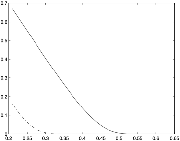
Figure 1: Probability of IBD at a single locus, as a function of $\beta$. Here, $L=10^{5}$, $\alpha=0.1$, $c_{L}=0.01$ and $\theta=10^{-3}$. The solid line corresponds to the case with small and large events, the dash–dot line to the case with only small events. Geographical correlations vanish around $\beta=0.32$ without large events, and are positive up to $\beta=0.52$ when large events occur.

Local bottlenecks are not the only explanations for a reduced effective population size. For example, selection or fluctuating population sizes can have the same effect, and so we should like to find a more “personal” signature of the presence of demographic events of different orders of magnitude. The idea that we explore here is to consider several loci on the same chromosome, subject to recombination, and to investigate the pattern of linkage disequilibrium obtained under the assumptions of Section 1.4. Using the results of Theorems 1.4 and 1.5, we have

$$\mathbb{P}_{L^{\beta}}[\mbox{IBD at both loci}]$$

$$\qquad=\mathbb{E}_{L^{\beta}}\bigl{[}e^{-2(\theta_{1}\tau_{Aa}^{L}+\theta_{2}\tau_{Bb}^{L})}\bigr{]}$$

$$\qquad\approx\mathbb{E}_{L^{\beta}}\bigl{[}e^{-2\theta_{1}\tau_{Aa}^{L}-2\theta_{2}\tau_{Bb}^{L}}\mathbf{1}_{\{c_{L}L^{2\beta}\leq\tau_{Aa}^{L}=\tau_{Bb}^{L}\leq c_{L}L^{2\gamma}\}}\bigr{]}$$

$$\qquad\quad{}+\mathbb{E}_{L^{\beta}}\bigl{[}e^{-2\theta_{1}\tau_{Aa}^{L}}\mathbf{1}_{\{\tau_{Aa}^{L}>c_{L}L^{2\gamma}\}}\bigr{]}\times\mathbb{E}_{L^{\beta}}\bigl{[}e^{-2\theta_{2}\tau_{Bb}^{L}}\mathbf{1}_{\{\tau_{Bb}^{L}>c_{L}L^{2\gamma}\}}\bigr{]},$$

where $\theta_{1}$ and $\theta_{2}$ denote the mutation rates at each locus and the first integral is $0$ if condition (2) holds (i.e., if there is no first period of complete correlation). By the same computations as in (2), the leading terms in this expression are

$$(\beta-\alpha)\int_{\beta}^{\gamma}\frac{e^{-2(\theta_{1}+\theta_{2})c_{L}L^{2u}}}{(u-\alpha)^{2}}\,du$$

(5)

$$\qquad{}+(\beta-\alpha)^{2}\biggl{(}\int_{\gamma}^{1}\frac{e^{-2\theta_{1}c_{L}L^{2u}}}{(u-\alpha)^{2}}\,du\biggr{)}\biggl{(}\int_{\gamma}^{1}\frac{e^{-2\theta_{2}c_{L}L^{2u}}}{(u-\alpha)^{2}}\,du\biggr{)}.$$

On the other hand, when there are no large events, the analysis of Lemma 4.3 (with effective recombination replaced by recombination and the separation to attain of the order of $L$) tells us that the time two lineages initially in the same individual need to “decorrelate” is of the order of $r_{L}^{-1}\log L$. Here $r_{L}^{-1}$ is the expected time to wait until we see a recombination event, and $\log L$ is (roughly) the mean number of recombination events before we see one after which the lineages remain separated for a duration $\mathcal{O}(L^{t})$ for some $t\in[\beta,1]$. Hence, when there are only small events, the leading terms in the probability of IBD at both loci are

$$\beta\int_{\beta}^{\gamma^{*}_{L}}\frac{e^{-2(\theta_{1}+\theta_{2})L^{2u}}}{u^{2}}\,du+\beta^{2}\biggl{(}\int_{\gamma^{*}_{L}}^{1}\frac{e^{-2\theta_{1}L^{2u}}}{u^{2}}\,du\biggr{)}\biggl{(}\int_{\gamma^{*}_{L}}^{1}\frac{e^{-2\theta_{2}L^{2u}}}{u^{2}}\,du\biggr{)},$$

where we have set $\gamma^{*}_{L}:=\log(r_{L}^{-1}\log L)/(2\log L)$ and the first integral is again zero if $\beta>\gamma^{*}_{L}$. Figure 2 compares the different curves obtained when (i) we always have decorrelation ($\gamma\leq\alpha$), (ii) we always have complete correlation ($\gamma\geq 1$), or (iii) when we have a transition between these two regimes [$\gamma\in(\alpha,1)$]. As expected, we see that the probability of IBD at both loci is higher in the presence of large events (when $\rho_{L}\leq L^{2\alpha}$), and there is correlation between the two loci when individuals are sampled over large spatial distances. Furthermore, (2) gives us an idea of how the correlations between the two loci decay with sampling distance, as this grows from the radius of the large events to the whole population range. Correlations for sampling distances smaller than or equal to the size of the large events will be the object of future work.

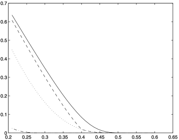
Figure 2: Probability of IBD at both loci, as a function of $\beta$. As in Figure 1, $L=10^{5}$, $\alpha=0.1$, $c_{L}=0.01$ and $\theta_{1}=\theta_{2}=10^{-3}$. The solid line corresponds to the case $\gamma\geq 1$ (complete correlation for any $\beta$), the dotted line to the case $\gamma\leq\alpha$ (decorrelation for any $\beta$) and the dashed line to the intermediate case $\gamma=0.4$. The dash–dot line corresponds to the case without large events, for which $\gamma_{L}^{*}$ is computed from the same parameter values (i.e., $\gamma_{L}^{*}=0.2$).

3 Genealogies at one locus

In this section we prove Proposition 1.2. In the process we introduce a rescaling of the spatial motion of our ancestral lineages and collect together several results on the time required to “gather” two lineages to within distance $2R_{B}L^{\alpha}$ which will also be needed in Section 4. Since the techniques mirror closely those used in previous work, in the interests of brevity, we restrict ourselves to sketching the proofs and providing references where appropriate.

Assume for the rest of this section that $\alpha<1$.

The following local central limit theorem, corresponding to Lemma 5.4 of BEV2010 , is the key to understanding the behavior of two lineages. Suppose that for each $L\in\mathbb{N}$, $\ell^{L}$ is a Lévy process on $\mathbb{T}(L)$ such that $\ell^{L}(1)-\ell^{L}(0)$ has a covariance matrix of the form $\sigma_{L}^{2}\operatorname{Id}$, and that: [(ii)]

there exists $\sigma^{2}>0$ such that $\sigma_{L}^{2}\rightarrow\sigma^{2}$ as $L\rightarrow\infty$;

$\mathrm{E}_{0}[|\ell^{L}(1)|^{4}]$ is bounded uniformly in $L$.

We shall implicitly suppose that all processes $\ell^{L}$ are defined on the same probability space, and that under the probability measure $\mathrm{P}_{x}$ the Lévy process we consider starts at $x$. Let $(d_{L})_{L\geq 1}$ be a sequence of positive reals such that $\liminf_{L\rightarrow\infty}d_{L}>0$ and $\frac{\log^{+}(d_{L})}{\log L}\rightarrow\eta\in[0,1)$. Finally, let us write $p^{L}(x,t)$ for $\mathrm{P}_{x}[\ell^{L}(t)\in B(0,d_{L})]$ and $\lfloor z\rfloor$ for the integer part of $z\in\mathbb{R}$.

Lemma A ((Lemma 5.4 in BEV2010 ))

Let $\varepsilon_{L}:=(\log L)^{-1/2}$. There exists a constant $C_{1}<\infty$ such that for every $L\geq 2$,

$$\sup_{t\geq\lfloor\varepsilon_{L}L^{2}\rfloor}\sup_{x\in\mathbb{T}(L)}\frac{\lfloor\varepsilon_{L}L^{2}\rfloor}{d_{L}^{2}}p^{L}(x,t)\leq C_{1}.$$

If $v_{L}\rightarrow\infty$ as $L\rightarrow\infty$, then

$$\lim_{L\rightarrow\infty}\sup_{t\geq\lfloor v_{L}L^{2}\rfloor}\sup_{x\in\mathbb{T}(L)}\frac{L^{2}}{d_{L}^{2}}\biggl{|}p^{L}(x,t)-\frac{\pi d_{L}^{2}}{L^{2}}\biggr{|}=0.$$

If $u_{L}\rightarrow\infty$ as $L\rightarrow\infty$ and $I(d_{L},x):=1+(|x|^{2}\vee d_{L}^{2})$, then

$$\lim_{L\rightarrow\infty}\sup_{x\in\mathbb{T}(L)}\sup_{u_{L}I(d_{L},x)\leq t\leq\varepsilon_{L}L^{2}}\frac{2\sigma_{L}^{2}t}{d_{L}^{2}}\biggl{|}p^{L}(x,t)-\frac{d_{L}^{2}}{2\sigma_{L}^{2}t}\biggr{|}=0.$$

There exists a constant $C_{2}<\infty$ such that for every $L\geq 1$,

$$\sup_{t\geq 0}\sup_{x\in\mathbb{T}(L)}\biggl{(}1+\frac{|x|^{2}}{d_{L}^{2}}\biggr{)}p^{L}(x,t)\leq C_{2}.$$

What Lemma A shows is that, for times which are large but of order at most $\mathcal{O}(L^{2})$, $\ell^{L}$ behaves like two-dimensional Brownian motion (case $c$), and, in particular, it has not yet explored the torus enough to “see” that space is limited. On the other hand, $\ell^{L}(t)$ is nearly uniformly distributed over $\mathbb{T}(L)$ at any time much greater than $L^{2}$ (case $b$).

Fix $R>0$. As a direct corollary of this local central limit theorem, we proved in Lemma 5.5 of BEV2010 that, if $T(R,\ell^{L})$ denotes the entrance time of $\ell^{L}$ into the ball $B(0,R)$, then the following inequality holds.

Lemma B ((Lemma 5.5 in BEV2010 ))

Let $(U_{L})_{L\geq 1}$ and $(u_{L})_{L\geq 1}$ be two sequences increasing to infinity such that $U_{L}L^{-2}\rightarrow\infty$ as $L\rightarrow\infty$ and $2u_{L}\leq L^{2}(\log L)^{-1/2}$ for every $L\geq 1$. Then, there exist $C_{0}>0$ and $L_{0}\in\mathbb{N}$ such that for every sequence $(U_{L}^{\prime})_{L\geq 1}$ satisfying $U_{L}^{\prime}\geq U_{L}$ for each $L$, every $L\geq L_{0}$ and all $x\in\mathbb{T}(L)$,

$$\mathrm{P}_{x}\bigl{[}T(R,\ell^{L})\in[U_{L}^{\prime}-u_{L},U_{L}^{\prime}]\bigr{]}\leq\frac{C_{0}u_{L}}{L^{2}}.$$

Lemma B tells us about the regime in which $\ell^{L}$ has already homogenized over $\mathbb{T}(L)$. Using exactly the same method, but employing parts (c) and (d) of Lemma A rather than (b), we obtain the analogous result for the regime in which $\ell^{L}$ behaves as Brownian motion on $\mathbb{R}^{2}$:

Lemma 3.1

If $U_{L}\leq L^{2}(\log L)^{-1/2}$ for each $L\geq 1$, $U_{L},u_{L}\rightarrow\infty$ and $u_{L}/U_{L}\rightarrow 0$ as $L\rightarrow\infty$, then there exist $C_{1}>0$ and $L_{1}\in\mathbb{N}$ such that for every sequence $(U_{L}^{\prime})_{L\geq 1}$ satisfying $U_{L}\leq U_{L}^{\prime}\leq L^{2}(\log L)^{-1/2}$ for each $L$, for every $L\geq L_{1}$ and $x\in\mathbb{T}(L)$,

$$\mathrm{P}_{x}\bigl{[}T(R,\ell^{L})\in[U_{L}^{\prime}-u_{L},U_{L}^{\prime}]\bigr{]}\leq\frac{C_{1}u_{L}}{U_{L}^{\prime}}.\vspace*{-2pt}$$

Let us now introduce the processes to which we wish to apply these results. For each $L\in\mathbb{N}$, let $\{\tilde{X}_{Aa}^{L}(t),t\geq 0\}$ be the process recording the difference between the locations on $\mathbb{T}(L)$ of the ancestral lineages of $A$ and $a$ (i.e., the first locus of each of the two individuals sampled). The process $\tilde{X}_{Aa}^{L}$ is the difference between two dependent compound Poisson processes. Under the probability measures we shall use, it is a Markov process (see Remark 3.2). Observe that, because the largest events have radius $R_{B}L^{\alpha}$, the lineages have to be within a distance less than $2R_{B}L^{\alpha}$ of each other to be hit by the same event. As a consequence, the law of $\tilde{X}_{Aa}^{L}$ outside $B(0,2R_{B}L^{\alpha})$ is equal to that of the difference $\tilde{Y}^{L}$ of two i.i.d. Lévy processes, each of which follows the evolution given in (1), and thus is also equal to the law of the motion of a single lineage run at twice the speed. We define the processes $X_{Aa}^{L}$ and $Y^{L}$ by

$$X_{Aa}^{L}(t)=\frac{1}{L^{\alpha}}\tilde{X}_{Aa}^{L}(\rho_{L}t)\quad\mbox{and}\quad Y^{L}(t)=\frac{1}{L^{\alpha}}\tilde{Y}^{L}(\rho_{L}t),\qquad t\geq 0,$$ (6)

both evolving on $\mathbb{T}(L^{1-\alpha})$. Using computations from the proof of Proposition 6.2 in BEV2010 and the jump intensities given in (1), we find that the covariance matrix of $Y^{L}(1)-Y^{L}(0)$ is the identity matrix multiplied by

$$2\biggl{\{}\frac{u_{s}\rho_{L}}{\pi R_{s}^{2}L^{2\alpha}}\int_{\mathbb{R}^{2}}(x_{1})^{2}L_{R_{s}}(x,0)\,dx+\frac{u_{B}}{\pi R_{B}^{2}}\int_{\mathbb{R}^{2}}(x_{1})^{2}L_{R_{B}}(x,0)\,dx\biggr{\}}+o(1)$$

$$\qquad=:2\sigma_{L}^{2}+o(1),$$

with $\sigma_{L}^{2}$ tending to a finite limit $\sigma^{2}>0$ as $L\rightarrow\infty$ (by our assumption on $L^{-2\alpha}\rho_{L}$). The $o(1)$ remainder here is the error we make by considering $\tilde{Y}^{L}$ as evolving on $\mathbb{R}^{2}$ instead of $\mathbb{T}(L)$ (see the proof of Proposition 6.2 in BEV2010 ). Assumption (ii) is also satisfied, and so Lemma A and its corollaries apply to $(Y^{L})_{L\geq 1}$, with the torus sidelength $L$ replaced by $L^{1-\alpha}$. Furthermore, $X_{Aa}^{L}$ and $Y^{L}$ follow the same evolution outside $B(0,2R_{B})$ for every $L$. This will be sufficient to prove Proposition 1.2: we shall show that the time the ancestral lineages of $A$ and $a$ need to coalesce once they are within distance $2R_{B}L^{\alpha}$ of one another [or, equivalently, once $X_{Aa}^{L}$ has entered $B(0,2R_{B})$] is negligible compared to the time they need to be gathered at distance $2R_{B}L^{\alpha}$. It is therefore the “gathering time” that dictates the coalescence time of two lineages starting at separation $|x_{L}|\gg L^{\alpha}$.

Remark 3.2.

It is here that we take advantage of the form of our recombination mechanism (recall Remark 1.1). When $\tilde{X}_{Aa}^{L}(t)\neq 0$, its future evolution is determined by the homogeneous Poisson point processes of events $\Pi_{B}^{L}$ and $\Pi_{s}^{L}$, and depends only on the current separation of the two lineages. If $\tilde{X}_{Aa}^{L}(t)=0$, the situation depends upon whether the two lineages are in the same individual (i.e., they have coalesced and will require a recombination event to separate again), or in two distinct individuals at the same spatial location. However, because of the form of our recombination mechanism, two lineages can jump onto the same location only if they are descendants of the same parent (in which case they necessarily coalesce). This means that provided we choose our initial condition in such a way that two lineages in the same spatial location are actually in the same individual, with probability one we will never see two lineages in distinct individuals but the same spatial location and so $\tilde{X}_{Aa}^{L}$ is indeed a Markov process under $\mathbb{P}_{a_{L}}$.

Notation 3.3.

As at the beginning of the section, we assume that all $Y^{L}$’s are defined on the same probability space, and start at $x$ under the probability measure $\mathrm{P}_{x}$. Since $X_{Aa}^{L}$ is a function of the genealogical process of $A,a,B$ and $b$, we retain the notation $\mathbb{P}_{a_{L}}$ when referring to it, and $X_{Aa}^{L}$ then starts a.s. at $L^{-\alpha}x_{L}$ if $x_{L}\in\mathbb{T}(L)$ is the initial separation between lineages $A$ and $a$.

The proof of Proposition 1.2 will require two subsidiary results. For each $L\in\mathbb{N}$, let $T_{Aa}^{L}$ be the first time the two lineages $A$ and $a$ are at separation less than $2R_{B}L^{\alpha}$. Equivalently, $\rho_{L}^{-1}T_{Aa}^{L}$ is the entrance time of $X_{Aa}^{L}$ into $B(0,2R_{B})$. By the observation made in the paragraph preceding Remark 3.2, $\rho_{L}^{-1}T_{Aa}^{L}$ under $\mathbb{P}_{a_{L}}$ has the same distribution as $T(2R_{B},Y^{L})$ under $\mathrm{P}_{L^{-\alpha}x_{L}}$, which yields the following lemma.

Lemma 3.4

Under the assumptions of Proposition 1.2, we have

$$\lim_{L\rightarrow\infty}\mathbb{P}_{a_{L}}\bigl{[}T_{Aa}^{L}>\rho_{L}L^{2(t-\alpha)}\bigr{]} = \frac{\beta-\alpha}{t-\alpha}\qquad\forall t\in[\beta,1]\quad\mbox{and}$$ (8)

$$\qquad\lim_{L\rightarrow\infty}\mathbb{P}_{a_{L}}\biggl{[}T_{Aa}^{L}>\frac{1-\alpha}{2\pi\sigma^{2}}\rho_{L}L^{2(1-\alpha)}\log Lt\biggr{]} = \frac{\beta-\alpha}{1-\alpha}e^{-t}\qquad\forall t>0.$$ (9)

Furthermore, for any $\beta_{0}\in(\alpha,1)$ and $\varepsilon>0$, the convergence in the first (resp., second) expression is uniform in $\beta,t\in[\beta_{0},1]$ (resp., $\beta\in[\beta_{0},1]$ and $t\geq\varepsilon$) and $a_{L}$ such that $|x_{L}|\in[L^{\beta}/(\log L),L^{\beta}\log L]$.

When $\beta=1$, the results are a weaker version of Proposition 6.2 in BEV2010 , in which the convergence in (9) is uniform over $t\geq 0$ and over the set of sequences $(x_{L})_{L\geq 1}$ such that $|x_{L}|\geq L(\log L)^{-1}$ for every $L$. Here, we relax the condition on $(x_{L})_{L\geq 1}$, but since the arguments in the proof of convergence (without requiring uniformity) only use the asymptotic behavior of $\log|x_{L}|$, they are still valid.

If $\beta<1$, the reasoning is the same as in the proofs of Lemma 3.6 in ZCD2005 (note that as above we allow more general sequences of initial separations at the expense of the uniformity of the convergence) and Theorem 2 in CD2002 . This does not come as a surprise, since the same local central limit theorem applies to both $Y^{L}$ [on $\mathbb{T}(L^{1-\alpha})$] and Zähle, Cox and Durrett’s $Y$ [on $\mathbb{T}(L)\cap\mathbb{Z}^{2}$] up to some constants depending on the geometry of the geographical patches considered. Hence, since $X_{Aa}^{L}$ starts from $L^{-\alpha}x_{L}$ and $\log(L^{-\alpha}|x_{L}|)/(\log L)\rightarrow\beta-\alpha$ by assumption, we can write (as in Lemma 3.6 of ZCD2005 )

$$\lim_{L\rightarrow\infty}\sup_{\beta\leq t\leq\kappa_{L}}\biggl{|}\mathbb{P}_{a_{L}}\bigl{[}T_{Aa}^{L}>\rho_{L}L^{2(t-\alpha)}\bigr{]}-\frac{\beta-\alpha}{t-\alpha}\biggr{|}$$

$$\qquad=\lim_{L\rightarrow\infty}\sup_{\beta\leq t\leq\kappa_{L}}\biggl{|}\mathrm{P}_{L^{-\alpha}x_{L}}\bigl{[}T(2R_{B},Y^{L})>L^{2(t-\alpha)}\bigr{]}-\frac{\beta-\alpha}{t-\alpha}\biggr{|}$$

$$\qquad=0,$$

where $\kappa_{L}=1-(\log\log L)/(2\log L)$ [so that $L^{2(\kappa_{L}-\alpha)}=L^{2(1-\alpha)}/(\log L)$]. Now, as in Lemma 3.8 of ZCD2005 , there exists $L_{0}\in\mathbb{N}$ and a constant $C$ such that, for every $L\geq L_{0}$ and $x\in\mathbb{T}(L)$,

$$\mathrm{P}_{x}\biggl{[}Y^{L}(s)=0\mbox{ for some }s\in\biggl{[}\frac{L^{2(1-\alpha)}}{\log L},L^{2(1-\alpha)}\biggr{]}\biggr{]}\leq\frac{C\log\log L}{\log L}.$$ (10)

Combining these two results, we obtain (8).

Finally, (9) is the analogue of Theorem 2 in CD2002 and can either be proved using the same technique or in the same way as Proposition 6.2 in BEV2010 (which, in addition, gives the appropriate constant in the time-rescaling). The uniform convergence stated in the second part of Lemma 3.4 follows from a direct application of the techniques of ZCD2005 and BEV2010 cited above.

The next result we need is the time that two lineages starting at separation at most $2R_{B}L^{\alpha}$ take to coalesce. Under our assumption that $(\rho_{L}L^{-2\alpha})_{L\geq 1}$ is bounded, Proposition 6.4(a) in BEV2010 applied with $\psi_{L}:=L^{\alpha}$ shows that for any sequence $(\phi_{L})_{L\geq 1}$ tending to infinity, we have

$$\lim_{L\rightarrow\infty}\sup_{a_{L}^{\prime}}\mathbb{P}_{a_{L}^{\prime}}[\tau_{Aa}^{L}>\phi_{L}\rho_{L}]=0,$$ (11)

where the supremum is taken over all configurations $a_{L}^{\prime}$ such that the distance between the blocks containing $A$ and $a$ is at most $2R_{B}L^{\alpha}$. Observe that in BEV2010 , only one individual reproduces during an event, and so if several lineages are affected by this event, they necessarily coalesce. Here, the distributions $\lambda_{s}$ and $\lambda_{B}$ of the number of potential parents are more general, but we assumed that their supports were compact. Thus, the probability that several individuals in the area of an event come from the same parent does not vanish as $L$ tends to infinity, which is all that we need to prove (11).

Remark 3.5.

Since (11) shows that coming to within $2R_{B}L^{\alpha}$ is almost equivalent to coalescing for two lineages, this is the only point where the distributions $\lambda_{s}$ and $\lambda_{B}$ appear in our discussion.

Proof of Proposition 1.2 Equipped with these results and the corollaries of Lemma A, we can now write for any given $t\in[\beta,1]$

$$\mathbb{P}_{a_{L}}\bigl{[}\tau_{Aa}^{L}>\rho_{L}L^{2(t-\alpha)}\bigr{]}$$

$$\qquad=\mathbb{P}_{a_{L}}\bigl{[}\tau_{Aa}^{L}>\rho_{L}L^{2(t-\alpha)};T_{Aa}^{L}>\rho_{L}\bigl{(}L^{2(t-\alpha)}-\log L\bigr{)}\bigr{]}$$ (12)

$$\qquad\quad{}+\mathbb{P}_{a_{L}}\bigl{[}\tau_{Aa}^{L}>\rho_{L}L^{2(t-\alpha)};T_{Aa}^{L}\leq\rho_{L}\bigl{(}L^{2(t-\alpha)}-\log L\bigr{)}\bigr{]}.$$

The second term on the right-hand side of (3) tends to zero by the strong Markov property applied at time $T_{Aa}^{L}$ and (11) with $\phi_{L}=\log L$. Then, we have, for each $L$,

$$\bigl{|}\mathbb{P}_{a_{L}}\bigl{[}\tau_{Aa}^{L}>\rho_{L}L^{2(t-\alpha)};T_{Aa}^{L}>\rho_{L}\bigl{(}L^{2(t-\alpha)}-\log L\bigr{)}\bigr{]}-\mathbb{P}_{a_{L}}\bigl{[}T_{Aa}^{L}>\rho_{L}L^{2(t-\alpha)}\bigr{]}\bigr{|}$$

$$\qquad\leq\mathbb{P}_{a_{L}}\bigl{[}\rho_{L}\bigl{(}L^{2(t-\alpha)}-\log L\bigr{)}\leq T_{Aa}^{L}\leq\rho_{L}L^{2(t-\alpha)}\bigr{]}$$

$$\qquad=\mathrm{P}_{L^{-\alpha}x_{L}}\bigl{[}L^{2(t-\alpha)}-\log L\leq T(2R_{B},Y^{L})\leq L^{2(t-\alpha)}\bigr{]},$$

which tends to zero by Lemma 3.1 applied with $L$ replaced by $L^{1-\alpha}$ (the size of the torus on which $Y^{L}$ evolves) if $t<1$, and by (10) if $t=1$. Lemma 3.4 enables us to deduce (a).

For (b), the same technique applies but with the last argument replaced by the use of Lemma B.

Proposition 1.2 is, in fact, a particular case of a more general result which we shall use in Section 4.3 (with $k=4$). Suppose we follow the ancestry at one locus of $k\geq 2$ different individuals. By analogy with above, we label individuals $1,\ldots,k$, we write $x_{ij}^{L}$ for the initial separation of lineages $i$ and $j$, $T_{ij}^{L}$ for the time at which their ancestral lineages first come within $2R_{B}L^{\alpha}$ and $\tau_{ij}^{L}$ for their coalescence time. We also write $T_{*}^{L}$ (resp., $\tau_{*}^{L}$) for the minimum over $\{i\neq j\}$ of the $T_{ij}^{L}$’s (resp., the $\tau_{ij}^{L}$’s). Although (in the same way as above) we could state a result for a more general sequence $(a_{L})_{L\geq 1}$ of initial configurations, for the proof of Theorem 1.4 we shall need some uniformity in the convergence. For this reason, we consider $\Gamma(L,k,\eta)$, the set of all configurations of $k$ lineages on $\mathbb{T}(L)$ such that all pairwise distances $|x_{ij}^{L}|$ belong to $[L^{\eta}/(\log L),L^{\eta}\log L]$.

Proposition 3.6

For any $\beta\in(\alpha,1]$, $\varepsilon>0$ and $i\neq j$, we have

$$\lim_{L\rightarrow\infty}\sup_{\beta\leq\eta\leq t\leq 1}\sup_{a_{L}\in\Gamma(L,k,\eta)}\biggl{|}\mathbb{P}_{a_{L}}\bigl{[}\tau_{*}^{L}=\tau_{ij}^{L}\leq\rho_{L}L^{2(t-\alpha)}\bigr{]}-\frac{1}{{k\choose 2}}\biggl{(}1-\biggl{(}\frac{\eta-\alpha}{t-\alpha}\biggr{)}^{{k}\choose{2}}\biggr{)}\biggr{|}$$

$$\qquad=0,$$

$$\lim_{L\rightarrow\infty}\sup_{t\geq\varepsilon,\beta\leq\eta\leq 1}\sup_{a_{L}\in\Gamma(L,k,\eta)}\biggl{|}\mathbb{P}_{a_{L}}\biggl{[}\tau_{*}^{L}=\tau_{ij}^{L}\leq\frac{1-\alpha}{2\pi\sigma^{2}}\rho_{L}L^{2(1-\alpha)}\log Lt\biggr{]}$$

$$\hskip 150.0pt\qquad{}-\frac{1}{{k\choose 2}}\biggl{(}1-\biggl{(}\frac{\eta-\alpha}{1-\alpha}e^{-t}\biggr{)}^{{k}\choose{2}}\biggr{)}\biggr{|}=0.$$

The same is true with $\tau^{L}$ replaced by $T^{L}$.

In essence, Proposition 3.6 tells us that on the timescale $\rho_{L}L^{2(t-\alpha)},t\in[\eta,1]$, the time of the first coalescence (or of the first “gathering”) is approximately the same as that of the first merger in a Kingman coalescent timechanged by $\log(\frac{t-\alpha}{\eta-\alpha})$, and that the approximation is uniform over $\eta$’s bounded away from $\alpha$. Moreover, asymptotically, just as in the Kingman coalescent, each pair of lineages has the same chance to be the first to coalesce. On the other hand, on the timescale $\frac{1-\alpha}{2\pi\sigma^{2}}\rho_{L}L^{2(1-\alpha)}\log Lt$, conditional on $T_{*}^{L}>\rho_{L}L^{2(1-\alpha)}$, the asymptotic behavior corresponds to Kingman’s coalescent run at speed $1$.

Sketch of proof The proof of Proposition 3.6 is a straightforward adaptation of those of Lemma 4.2 and of Lemma 5.2 in ZCD2005 (see also the comments given in the paragraph following the proof of Lemma 4.2). The interested reader will also find there references to earlier results for the random walks with instantaneous coalescence which are dual to the two-dimensional voter model.

Let us end this section by recalling a lemma of BEV2010 and by stating an analogous result. For every $L\in\mathbb{N}$, $i\neq j$ and $t\geq 0$, let $\tilde{X}_{ij}^{L}(t)$ be the separation [on $\mathbb{T}(L)$ at time $t$] of lineages $i$ and $j$.

Lemma C ((Lemma 6.9 in BEV2010 ))

Suppose $k=4$ and

$$\lim_{L\rightarrow\infty}\frac{\min_{i\neq j}\log|x_{ij}^{L}|}{\log L}=\lim_{L\rightarrow\infty}\frac{\max_{i\neq j}\log|x_{ij}^{L}|}{\log L}=1.$$ (13)

Then,

$$\lim_{L\rightarrow\infty}\mathbb{P}_{a_{L}}\biggl{[}\tau_{*}^{L}=\tau_{12}^{L};|\tilde{X}_{13}^{L}(\tau_{*}^{L})|\leq\frac{L}{\log L}\biggr{]} = 0,$$

$$\lim_{L\rightarrow\infty}\mathbb{P}_{a_{L}}\biggl{[}\tau_{*}^{L}=\tau_{12}^{L};|\tilde{X}_{34}^{L}(\tau_{*}^{L})|\leq\frac{L}{\log L}\biggr{]} = 0.$$

These results are also true if $\tau^{L}$ is replaced by $T^{L}$.

In words, when two lineages meet and coalesce, with probability tending to one the others are at distance at least $L/\log L$ of each other and of the coalescing pair (in particular, such a merger involves at most two lineages at a time). When the initial distance between the lineages is of the order of $L^{\beta}$ with $\beta<1$, we have instead:

Lemma 3.7

Suppose again $k=4$ and the limit in (13) is equal to $\beta\in(\alpha,1)$. Then,

$$\lim_{L\rightarrow\infty}\mathbb{P}_{a_{L}}\biggl{[}\tau_{*}^{L}=\tau_{12}^{L}\leq\frac{\rho_{L}L^{2(1-\alpha)}}{\log L};|\tilde{X}_{13}^{L}(\tau_{*}^{L})|\notin\biggl{[}\frac{L^{\alpha}}{\log L}\frac{\sqrt{\tau_{*}^{L}}}{\sqrt{\rho_{L}}},L^{\alpha}\log L\frac{\sqrt{\tau_{*}^{L}}}{\sqrt{\rho_{L}}}\biggr{]}\biggr{]}$$

$$\qquad=0,$$

$$\lim_{L\rightarrow\infty}\mathbb{P}_{a_{L}}\biggl{[}\tau_{*}^{L}=\tau_{12}^{L}\leq\frac{\rho_{L}L^{2(1-\alpha)}}{\log L};|\tilde{X}_{34}^{L}(\tau_{*}^{L})|\notin\biggl{[}\frac{L^{\alpha}}{\log L}\frac{\sqrt{\tau_{*}^{L}}}{\sqrt{\rho_{L}}},L^{\alpha}\log L\frac{\sqrt{\tau_{*}^{L}}}{\sqrt{\rho_{L}}}\biggr{]}\biggr{]}$$

$$\qquad=0.$$

The result is also true if $\tau^{L}$ is replaced by $T^{L}$.

Notice the rescalings of time by $\rho_{L}$ and space by $L^{\alpha}$ introduced in (6) under which the behavior of the lineages is close to that of finite variance random walks. In fact, although their formulations are rather different, Lemma 3.7 is very similar to Lemma 1 in CG1986 or Lemma 5.1 in ZCD2005 for coalescing random walks.

Sketch of proof of Lemma 3.7 The method of proof is identical to that of Lemma 6.9 in BEV2010 , to which we refer for more complete arguments. It is based on two facts. First, by time $\rho_{L}L^{2(1-\alpha)}/(\log L)$ the separation of the lineages is never on the order of the side of the torus. Second, if $T_{*}^{L}=T_{12}^{L}$, then $L^{-\alpha}\tilde{X}_{13}^{L}(\rho_{L}\cdot)$ and $L^{-\alpha}\tilde{X}_{34}^{L}(\rho_{L}\cdot)$, considered separately, follow the same law as the difference of two independent lineages (on $\mathbb{R}^{2}$, by the first fact) conditioned on not entering $B(0,2R_{B})$ before $T_{*}^{L}/\rho_{L}$. By Lemma 3.4, with high probability $T_{*}^{L}/\rho_{L}\gg L^{2(\beta-\alpha)}$, and so the result for $T^{L}$ follows from a standard central limit theorem.

The modifications needed for $\tau^{L}$ use the very rapid coalescence of two lineages gathered at distance $2R_{B}L^{\alpha}$ to obtain that, with probability tending to $1$, if $\tau_{*}^{L}=\tau_{12}^{L}$, then no other pairs of lineages come within $2R_{B}L^{\alpha}$ of one another before time $\tau_{*}^{L}$. An application of Lemma 3.7 (with $T^{L}$) completes the proof.

4 Genealogies at two loci

From now on, we work with the rescaling of time and space introduced in (6). As we saw in the previous section, these are the appropriate scales on which to understand the behavior of a collection of independent processes following the dynamics driven by (1). Because our lineages move independently as long as they are at distance greater than $2R_{B}$ (in rescaled units) of each other, it is also the relevant regime in which to understand “gathering” and coalescence of ancestral lineages.

The aim of Sections 4.1 and 4.2 is to understand how two lineages, initially present in the same individual, can “decorrelate” and how much time they need to do so. Once this phenomenon is understood for two lineages, we can consider the more complex situation described in the Section 1.4 and prove Theorems 1.4 and 1.5. This is achieved in Section 4.3.

4.1 Effective recombination time

For every $L$, let $X_{AB}^{L}$ be the process that records the (rescaled) difference between the locations of the lineages labeled $A$ and $B$. Recall that under our working assumptions, these lineages start within the same individual (in other words, $A$ and $B$ belong to the same block of the marked partition $a_{L}$).

By construction, recombination occurs only during small events. In our rescaled space and time units, a recombination event results in a separation of the lineages of $\mathcal{O}(L^{-\alpha})$, and then small events affect them at rate $\mathcal{O}(\rho_{L})$. Hence, it is very likely that (in our rescaled time units) the lineages very rapidly coalesce and have to wait for the next recombination event [i.e., roughly $(\rho_{L}r_{L})^{-1}$ units of rescaled time] to be geographically separated again, and so on. An efficient way for the lineages to escape this “flickering” due to small events is for a large event to send them to a separation of $\mathcal{O}(1)$. This necessarily occurs at a time when $X_{AB}^{L}\neq 0$. Thus, let us define $S^{L}$ as the first time $t$ at which at least one of the two lineages is affected by a large event and $X_{AB}^{L}(t-)\neq 0$ [which does not prohibit $X_{AB}^{L}(t)=0$]. We call $S^{L}$ the effective recombination time. Its large-$L$ behavior is given by the following proposition.

Proposition 4.1

There exist $\theta_{1},\theta_{2}>0$ such that for every $\theta>\theta_{2}$ and every nonvanishing sequence $(\phi_{L})_{L\geq 1}$ satisfying $\phi_{L}\leq L^{2}/(\rho_{L}\log L)$ for every $L$, we have for $L$ large enough

$$\mathbb{P}_{a_{L}}\biggl{[}S^{L}\geq\phi_{L}\biggl{(}1+\frac{\theta\log(\phi_{L}\rho_{L})}{r_{L}\rho_{L}}\biggr{)}\biggr{]}\leq e^{-\theta_{1}\phi_{L}}+e^{-(\theta-\theta_{2})\phi_{L}\log(\phi_{L}\rho_{L})}.$$

The idea of the proof of Proposition 4.1 is to show that, with very high probability, the number of visits to $0$ of $X_{AB}^{L}$ before it has accumulated a time $\phi_{L}$ outside $0$ is less than $\phi_{L}\log(\phi_{L}\rho_{L})$. Since each visit lasts a time proportional to $(r_{L}\rho_{L})^{-1}$, the total amount of time it takes for $X_{AB}^{L}$ to accumulate $\phi_{L}$ units of time outside zero is at most of the order of $\phi_{L}+\phi_{L}\log(\phi_{L}\rho_{L})/(r_{L}\rho_{L})$. The probability that by this time the two lineages have not been affected by a large event while in distinct locations is bounded by a quantity of the form $e^{-C\phi_{L}}$.

Let us write $\mathcal{R}_{L}(x)$ for the rate at which at least one of the lineages is affected by a large event when $X_{AB}^{L}=x$, and recall that time is rescaled by a factor $\rho_{L}$. From the expression for the intensity of $\Pi_{B}^{L}$, we can find a constant $C_{B}>0$ such that $\mathcal{R}_{L}(x)\geq C_{B}$ for all $x\in\mathbb{T}(L^{1-\alpha})\setminus\{0\}$ [in fact, one can even show that the function $x\mapsto\mathcal{R}_{L}(x)$ is increasing in $|x|$, and so one can take $C_{B}:=\mathcal{R}_{L}(0)>0$]. Let $\hat{X}^{L}$ be a $\mathbb{T}(L^{1-\alpha})$-valued Markov process distributed in the same way as the difference between two lineages subject only to the events of $\Pi_{s}^{L}$, and $\hat{S}^{L}$ be an exponential random variable with instantaneous rate $\mathcal{R}_{L}(\hat{X}^{L}(t))\mathbf{1}_{\{\hat{X}^{L}(t)\neq 0\}}$. By the preceding remark, $\hat{S}^{L}$ is stochastically bounded by an exponential random variable with instantaneous rate $C_{B}\mathbf{1}_{\{\hat{X}^{L}(t)\neq 0\}}$. Because large events have no effect when $X_{AB}^{L}=0$, the law of the stopped process $\{X_{AB}^{L}(t),t\in[0,S^{L}]\}$ is the same as that of $\{\hat{X}^{L}(t),t\in[0,\hat{S}^{L}]\}$. Thus, for the proof of Proposition 4.1 we work with $\hat{X}^{L}$ and $\hat{S}^{L}$ and use $\mathrm{P}_{x}$ to denote the law of $\hat{X}^{L}$ under which $\mathbb{P}[\hat{X}^{L}(0)=x]=1$.

For each $L\in\mathbb{N}$, let us define the stopping times $(\hat{Q}_{i}^{L})_{i\geq 0}$ and $(\hat{q}_{i}^{L})_{i\geq 0}$ by $\hat{Q}_{0}^{L}=\hat{q}_{0}^{L}=0$ and for every $i\geq 1$,

$$\hat{Q}_{i}^{L} := \inf\{t\geq\hat{q}_{i-1}^{L}\dvtx\hat{X}^{L}(t)\neq 0\},$$

$$\hat{q}_{i}^{L} := \inf\{t\geq\hat{Q}_{i}^{L}\dvtx\hat{X}^{L}(t)=0\}.$$

[Note that $\hat{Q}_{1}^{L}=0$ if $\hat{X}^{L}(0)\neq 0$, in which case $\hat{q}_{1}^{L}$ is the first hitting time of $0$.] By construction, the random variables $(\hat{Q}_{i}^{L}-\hat{q}_{i-1}^{L})_{i\in\mathbb{N}}$ are i.i.d. and distributed according to an exponential random variable with parameter $C_{\mathrm{rec}}r_{L}\rho_{L}$, where $C_{\mathrm{rec}}:=\pi R_{s}^{2}u_{s}(1-\lambda_{s}(\{1\}))>0$ (the last factor arises since the number of reproducing individuals needs to be greater than one for recombination to occur). We have the following result for the excursions of $\hat{X}^{L}$ away from $0$.

Lemma 4.2

There exist $C_{e}>0$ and $u_{e}>0$ such that for every $L\geq 1$ and $u_{e}\leq u\leq L^{2}/(\log L)$, for every $x\in B(0,2R_{s}L^{-\alpha})\setminus\{0\}$,

$$\mathrm{P}_{x}[\hat{q}_{1}^{L}>u\rho_{L}^{-1}]\geq\frac{C_{e}}{\log u}.$$

Here (and only here) it is easier to work with the initial time and space units and show that the probability of an excursion outside $0$ of length greater than $u$ is bounded from below by $C_{e}/(\log u)$ when $u$ is large. Let us thus define $\tilde{X}^{L}$ by $\tilde{X}^{L}(t):=L^{\alpha}\hat{X}^{L}(\rho_{L}^{-1}t)$ for all $t\geq 0$, with the understanding that $\tilde{X}^{L}$ starts at $L^{\alpha}x$ under the probability measure $\mathrm{P}_{x}$.

The desired result is shown in RR1966 for standard discrete space random walks whose jumps have finite variance as well as for Brownian motion (with the hitting time of $0$ replaced by the entrance time into a ball of fixed radius) in two dimensions. To see why it is true for $\tilde{X}^{L}$ on $\mathbb{T}(L)$, observe first that by time $L^{2}/(\log L)$, the process $\tilde{X}^{L}$ does not see that space is limited, and so it behaves as though it were moving in $\mathbb{R}^{2}$. More precisely, there exists a constant $C>0$ such that for all $z\in B(0,6R_{s}L^{-\alpha})$,

$$\mathrm{P}_{z}\biggl{[}\sup_{u\leq L^{2}/(\log L)}|\tilde{X}^{L}(u)|>\frac{L}{3}\biggr{]}\leq\frac{C}{\log L}.$$

(Use the $L^{2}$-maximal inequality and the fact that $|\tilde{X}^{L}|$ is bounded by the corresponding quantity for the same process defined on $\mathbb{R}^{2}$, which is proportional to $L^{2}/(\log L)$ by equation (22) in BEV2010 ). Hence, let us assume that $\tilde{X}^{L}$ is defined on $\mathbb{R}^{2}$ instead of $\mathbb{T}(L)$. Since the evolution due to small events depends on $L$ only through the torus sidelength, with our new convention all $\tilde{X}^{L}$’s have the same distribution and we can drop the exponent $L$ in the notation. For the same reason, we also write $\tilde{q}_{1}$ for the random times $\rho_{L}\hat{q}_{1}^{L}$, that is, the length of the first excursion outside $0$ of $\tilde{X}$.

Let $\tilde{\mathrm{T}}_{(4R_{s})}$ denote the first time $\tilde{X}$ leaves $B(0,4R_{s})$ [and so $\tilde{X}(\tilde{\mathrm{T}}_{(4R_{s})})\in B(0,6R_{s})\setminus B(0,4R_{s})$ by our assumption on the jump sizes], and let $\tilde{\mathrm{T}}_{[2R_{s}]}$ be the first return time of $\tilde{X}$ into $B(0,2R_{s})$ after $\tilde{\mathrm{T}}_{(4R_{s})}$. We have for every $x\in B(0,2R_{s}L^{-\alpha})\setminus\{0\}$,

$$\mathrm{P}_{x}[\tilde{q}_{1}>u]$$

$$\qquad\geq\mathrm{P}_{x}\bigl{[}\tilde{q}_{1}>u;\tilde{\mathrm{T}}_{(4R_{s})}<\tilde{q}_{1}\bigr{]}$$

$$\qquad\geq\mathrm{P}_{x}\bigl{[}\tilde{q}_{1}-\tilde{\mathrm{T}}_{(4R_{s})}>u;\tilde{\mathrm{T}}_{(4R_{s})}<\tilde{q}_{1}\bigr{]}$$

(14)

$$\qquad=\mathrm{E}_{x}\Bigl{[}\mathbf{1}_{\{\tilde{\mathrm{T}}_{(4R_{s})}<\tilde{q}_{1}\}}\mathrm{P}_{\tilde{X}(\tilde{\mathrm{T}}_{(4R_{s})})}[\tilde{q}_{1}>u]\Bigr{]}$$

$$\qquad\geq\mathrm{E}_{x}\bigl{[}\mathbf{1}_{\{\tilde{\mathrm{T}}_{(4R_{s})}<\tilde{q}_{1}\}}\mathrm{P}_{\tilde{X}(\tilde{\mathrm{T}}_{(4R_{s})})}\bigl{[}\tilde{\mathrm{T}}_{[2R_{s}]}>u\bigr{]}\bigr{]}$$

$$\qquad\geq\Bigl{(}\inf_{B(0,2R_{s})\setminus\{0\}}\mathrm{P}_{L^{-\alpha}y}\bigl{[}\tilde{\mathrm{T}}_{(4R_{s})}<\tilde{q}_{1}\bigr{]}\Bigr{)}\Bigl{(}\inf_{B(0,6R_{s})\setminus B(0,4R_{s})}\mathrm{P}_{L^{-\alpha}z}\bigl{[}\tilde{\mathrm{T}}_{[2R_{s}]}>u\bigr{]}\Bigr{)}.$$

The first infimum is strictly positive. To see this, note that $\mathrm{P}_{L^{-\alpha}y}[\tilde{\mathrm{T}}_{(4R_{s})}<\tilde{q}_{1}]$ is bounded from below by the probability that the first four small events affecting the lineages send them to a distance at least $4R_{s}$ of each other before they coalesce, and the infimum over $B(0,2R_{s})\setminus\{0\}$ of the latter probability is positive since $u_{s}<1$ (if $u_{s}=1$, only one of the lineages can be in the geographical range of such separating events, and so their probability of occurrence shrinks to $0$ as $|y|\rightarrow 0$).

For the second infimum in (4.1), we use the same construction as in the proof of Skorokhod embedding (see, e.g., BIL1995 ) to write the path of $\tilde{X}$ as that of a standard Brownian motion $W$ considered at particular times. More precisely, if $(\tilde{\sigma}_{i})_{i\in\mathbb{N}}$ is the sequence of jump times of $\tilde{X}$, we can find a sequence of Brownian stopping times $(\sigma_{i})_{i\in\mathbb{N}}$ such that $(W(\sigma_{i}))_{i\geq 0}$ has the same joint distributions as $(\tilde{X}(\tilde{\sigma}_{i}))_{i\geq 0}$. For every $i\in\mathbb{N}$, conditional on $W(\sigma_{i-1})$, $\sigma_{i}$ is the first time greater than $\sigma_{i-1}$ at which $W$ leaves $B(W(\sigma_{i-1}),l_{i})$, where the random variable $l_{i}$ is independent of $W$ and of $\{\sigma_{j},j<i\}$ and has the same distribution as the length of the first jump of $\tilde{X}$. As a consequence, if $\tilde{n}(u):=\max\{i\dvtx\tilde{\sigma}_{i}\leq u\}$, by comparing the paths of $\tilde{X}$ and of $W$ we obtain

$$\mathrm{P}_{L^{-\alpha}z}\bigl{[}\tilde{\mathrm{T}}_{[2R_{s}]}>u\bigr{]}\geq\mathrm{P}_{z}\bigl{[}W(t)\notin B(0,2R_{s}),\forall t\leq\sigma_{\tilde{n}(u)}\bigr{]}.$$

Now, each $\tilde{\sigma}_{i}-\tilde{\sigma}_{i-1}$ is stochastically bounded from below by an exponential random variable with positive parameter $k_{1}>0$, and so by standard large deviation results we can find $k_{2}>0$ large enough and $k_{3}>0$ such that for all $u>1$ and $y\in\mathbb{R}^{2}$,

$$\mathrm{P}_{y}[\tilde{n}(u)>k_{2}u]\leq e^{-k_{3}u}.$$

By construction, each $\sigma_{i}-\sigma_{i-1}$ is stochastically bounded from above by the first time Brownian motion started at $0$ leaves $B(0,2R_{s})$, which also has an exponential moment. Hence, there exist $k_{4},k_{5}>0$ such that for all $u>1$ and $y\in\mathbb{R}^{2}$,

$$\mathrm{P}_{y}\bigl{[}\sigma_{\lfloor k_{2}u\rfloor+1}>k_{4}u\bigr{]}\leq e^{-k_{5}u}.$$

Using these bounds and the result already established in RR1966 for Brownian motion at time $k_{4}u$, Lemma 4.2 is proved.

We now have all the ingredients we require to prove Proposition 4.1.

Proof of Proposition 4.1 Set

$$\psi_{L}:=\phi_{L}\biggl{(}1+\frac{\theta\log(\phi_{L}\rho_{L})}{r_{L}\rho_{L}}\biggr{)},$$ (15)

and call $\mathbf{t}(\psi_{L})$ the time $\hat{X}^{L}$ spends away from $0$ before time $\psi_{L}$. We have, for every $L$,

$$\mathrm{P}_{0}[\hat{S}^{L}\geq\psi_{L}] = \mathrm{P}_{0}[\hat{S}^{L}\geq\psi_{L};\mathbf{t}(\psi_{L})\leq\phi_{L}]+\mathrm{P}_{0}[\hat{S}^{L}\geq\psi_{L};\mathbf{t}(\psi_{L})>\phi_{L}]$$

$$\leq \mathrm{P}_{0}[\mathbf{t}(\psi_{L})\leq\phi_{L}]+e^{-C_{B}\phi_{L}},$$

where $C_{B}$ is the lower bound on the rate of effective large events introduced just below the statement of the proposition. Next, if we set $\hat{k}_{L}:=\sup\{i\dvtx\hat{Q}_{i}^{L}\leq\psi_{L}\}$, that is, $\hat{k}_{L}$ is the number of excursions of $\hat{X}^{L}$ away from $0$ which start before time $\psi_{L}$, we can write

$$\mathrm{P}_{0}[\mathbf{t}(\psi_{L})\leq\phi_{L}] = \mathrm{P}_{0}[\mathbf{t}(\psi_{L})\leq\phi_{L};\hat{k}_{L}\leq\phi_{L}\log(\phi_{L}\rho_{L})]$$

$${}+\mathrm{P}_{0}[\mathbf{t}(\psi_{L})\leq\phi_{L};\hat{k}_{L}>\phi_{L}\log(\phi_{L}\rho_{L})].$$

On the one hand,

$$\mathrm{P}_{0}[\mathbf{t}(\psi_{L})\leq\phi_{L};\hat{k}_{L}>\phi_{L}\log(\phi_{L}\rho_{L})] \leq \mathrm{P}_{0}\Biggl{[}\sum_{i=1}^{\lfloor\phi_{L}\log(\phi_{L}\rho_{L})\rfloor}(\hat{q}_{i}^{L}-\hat{Q}_{i}^{L})\leq\phi_{L}\Biggr{]}$$

$$\leq \mathrm{P}_{0}[\hat{q}_{1}^{L}-\hat{Q}_{1}^{L}\leq\phi_{L}]^{\lfloor\phi_{L}\log(\phi_{L}\rho_{L})\rfloor}$$

$$\leq \biggl{(}1-\frac{C_{e}}{\log(\phi_{L}\rho_{L})}\biggr{)}^{\lfloor\phi_{L}\log(\phi_{L}\rho_{L})\rfloor}$$

$$\leq e^{-C_{e}^{\prime}\phi_{L}},$$

for a constant $C_{e}^{\prime}>0$ and $L$ large enough. The second line is obtained by an obvious recursion using the strong Markov property at the successive times $\hat{q}_{i}^{L}$ in decreasing order, and the third line uses Lemma 4.2 [recall that by assumption on $\phi_{L}$, we have $\phi_{L}\rho_{L}\rightarrow\infty$ and $\phi_{L}\rho_{L}\leq L^{2}/(\log L)$]. Hence, we can set $\theta_{1}:=C_{B}\wedge C_{e}^{\prime}$. On the other hand,

$$\mathrm{P}_{0}[\mathbf{t}(\psi_{L})\leq\phi_{L};\hat{k}_{L}\leq\phi_{L}\log(\phi_{L}\rho_{L})]$$

$$\qquad\leq\mathrm{P}_{0}\Biggl{[}\sum_{i=1}^{\lfloor\phi_{L}\log(\phi_{L}\rho_{L})\rfloor+1}(\hat{Q}_{i}^{L}-\hat{q}_{i-1}^{L})\geq\psi_{L}-\phi_{L}\Biggr{]}$$

$$\qquad=\mathrm{P}_{0}\Biggl{[}\exp\Biggl{\{}r_{L}\rho_{L}\sum_{i=1}^{\lfloor\phi_{L}\log(\phi_{L}\rho_{L})\rfloor+1}(\hat{Q}_{i}^{L}-\hat{q}_{i-1}^{L})\Biggr{\}}\geq\exp\{r_{L}\rho_{L}(\psi_{L}-\phi_{L})\}\Biggr{]}$$

$$\qquad\leq e^{-\theta\phi_{L}\log(\phi_{L}\rho_{L})}\mathrm{E}_{0}\Biggl{[}\exp\Biggl{\{}r_{L}\rho_{L}\sum_{i=1}^{\lfloor\phi_{L}\log(\phi_{L}\rho_{L})\rfloor+1}(\hat{Q}_{i}^{L}-\hat{q}_{i-1}^{L})\Biggr{\}}\Biggr{]},$$

where the last line uses the Markov inequality. As we pointed out above, the random variables $r_{L}\rho_{L}(\hat{Q}_{i}^{L}-\hat{q}_{i-1}^{L})$ are i.i.d. with law $\operatorname{Exp}(C_{\mathrm{rec}})$. Therefore, we can write for a constant $\theta_{2}>0$

$$\mathrm{P}_{0}[\mathbf{t}(\psi_{L})\leq\phi_{L};\hat{k}_{L}\leq\phi_{L}\log(\phi_{L}\rho_{L})]\leq e^{-(\theta-\theta_{2})\phi_{L}\log(\phi_{L}\rho_{L})}.$$

Combining these results, the proof of Proposition 4.1 is complete.

Finally, let us use Proposition 4.1 to obtain some estimates on the time two lineages starting in the same individual need to reach a separation at which they start to evolve independently. The following lemma will be a key result for the proof of Proposition 4.4 in the next section. For every $L\in\mathbb{N}$, let $\mathrm{T}_{(3R_{B})}^{L}$ denote the exit time of $X_{AB}^{L}$ from $B(0,3R_{B})$.

Lemma 4.3

There exists a constant $\theta_{3}>0$ such that if $(\phi_{L})_{L\geq 1}$ is as in Proposition 4.1, $\phi_{L}\rightarrow\infty$ as $L\rightarrow\infty$ and $\theta>\theta_{2}$, there exists $L_{0}=L_{0}(\theta,(\phi_{L})_{L\in\mathbb{N}})$ such that for every $L\geq L_{0}$,

$$\mathbb{P}_{a_{L}}\biggl{[}\mathrm{T}_{(3R_{B})}^{L}\geq\phi_{L}\biggl{(}1+\frac{\theta\log(\phi_{L}\rho_{L})}{r_{L}\rho_{L}}\biggr{)}\biggr{]}\leq\sqrt{\phi_{L}}e^{-\theta_{3}\sqrt{\phi_{L}}}.$$

For conciseness, we again use the notation $\psi_{L}$ introduced in (15). This time we define $Q_{0}^{L}=q_{0}^{L}=0$ and

$$Q_{i}^{L} := \inf\{t>q_{i-1}^{L}\dvtx t\mbox{ is the epoch of an effective recombination}\},$$

$$q_{i}^{L} := \inf\{t\geq Q_{i}^{L}\dvtx X_{AB}^{L}(t)=0\mbox{ or }X_{AB}^{L}(t)\notin B(0,3R_{B})\},$$

$$k_{L} := \max\bigl{\{}i\dvtx Q_{i}^{L}\leq\mathrm{T}_{(3R_{B})}^{L}\bigr{\}}.$$

First, we claim that there exists a constant $\wp>0$ independent of $L$ such that, for $L$ large enough, $k_{L}+1$ is stochastically bounded by a geometric random variable with success probability $\wp$. In other words, the probability that $X_{AB}^{L}$ starting at $x\in B(0,3R_{B})\setminus\{0\}$ leaves $B(0,3R_{B})$ before hitting $0$ is bounded from below by $\wp$, independently of $x$. The proof of this claim is given in the first paragraph of the proof of Lemma 6.6 in BEV2010 . (The quantity $\wp$ is taken to be the probability that a sequence of large events sends the lineages to a distance of at least $3R_{B}$ without meanwhile being counteracted by small events bringing them too close together.) As a consequence, for any large $L$,

$$\mathbb{P}_{a_{L}}\bigl{[}\mathrm{T}_{(3R_{B})}^{L}\geq\psi_{L}\bigr{]}\leq\mathbb{P}_{a_{L}}\bigl{[}\mathrm{T}_{(3R_{B})}^{L}\geq\psi_{L};k_{L}<\sqrt{\phi_{L}}\bigr{]}+(1-\wp)^{\sqrt{\phi_{L}}}.$$

Next, let us write

$$\mathbb{P}_{a_{L}}\bigl{[}\mathrm{T}_{(3R_{B})}^{L}\geq\psi_{L};k_{L}<\sqrt{\phi_{L}}\bigr{]}$$

(16)

$$\qquad=\mathbb{P}_{a_{L}}\Biggl{[}\mathrm{T}_{(3R_{B})}^{L}\geq\psi_{L};k_{L}<\sqrt{\phi_{L}};\sum_{i=1}^{k_{L}}(Q_{i}^{L}-q_{i-1}^{L})\geq\frac{\psi_{L}}{2}\Biggr{]}$$

$$\qquad\quad{}+\mathbb{P}_{a_{L}}\Biggl{[}\mathrm{T}_{(3R_{B})}^{L}\geq\psi_{L};k_{L}<\sqrt{\phi_{L}};\sum_{i=1}^{k_{L}}(Q_{i}^{L}-q_{i-1}^{L})<\frac{\psi_{L}}{2}\Biggr{]}.$$ (17)

The quantity in (4.1) is bounded by

$$\mathbb{P}_{a_{L}}\Biggl{[}\sum_{i=1}^{\lfloor\sqrt{\phi_{L}}\rfloor}(Q_{i}^{L}-q_{i-1}^{L})\geq\frac{\psi_{L}}{2}\Biggr{]} = 1-\mathbb{P}_{a_{L}}\Biggl{[}\sum_{i=1}^{\lfloor\sqrt{\phi_{L}}\rfloor}(Q_{i}^{L}-q_{i-1}^{L})<\frac{\psi_{L}}{2}\Biggr{]}$$

$$\leq 1-\mathbb{P}_{a_{L}}\biggl{[}\forall i\leq\lfloor\sqrt{\phi_{L}}\rfloor,Q_{i}^{L}-q_{i-1}^{L}<\frac{\psi_{L}}{2\sqrt{\phi_{L}}}\biggr{]}$$

$$\leq 1-\biggl{(}1-\sup_{a_{L}^{\prime}}\mathbb{P}_{a_{L}^{\prime}}\biggl{[}S^{L}\geq\frac{\psi_{L}}{2\sqrt{\phi_{L}}}\biggr{]}\biggr{)}^{\lfloor\sqrt{\phi_{L}}\rfloor},$$

where the last line is obtained by recursion (notice that, conditionally on $q_{i-1}^{L}$, $Q_{i}^{L}-q_{i-1}^{L}$ has the same law as the effective recombination time $S_{L}$) and the supremum is taken over all initial configurations $a_{L}^{\prime}$ in which lineages $A$ and $B$ are either at distance $0$ or at distance greater than $3R_{B}$. We can in fact restrict our attention to the set of configurations in which $A$ and $B$ belong to the same block. Indeed, if $|X_{AB}^{L}(0)|>3R_{B}$, we can decompose the probability that $S^{L}\geq\psi_{L}/(2\sqrt{\phi_{L}})$ into the sum of:

• the probability that $S^{L}\geq\psi_{L}/(2\sqrt{\phi_{L}})$ and $X_{AB}^{L}$ does not hit $0$ before time $\psi_{L}/(4\sqrt{\phi_{L}})$, which decreases like $e^{-C\psi_{L}/\sqrt{\phi_{L}}}$ since the rate at which large events affect the lineages when $X_{AB}^{L}\neq 0$ is bounded from below by a positive constant;

• the probability that $S^{L}\geq\psi_{L}/(2\sqrt{\phi_{L}})$ and $X_{AB}^{L}$ hits $0$ before time $\psi_{L}/\break(4\sqrt{\phi_{L}})$, which boils down to the case $X_{AB}^{L}(0)=0$ by the strong Markov property applied at the first time $X_{AB}^{L}=0$.

Now, by Proposition 4.1 applied with $\phi_{L}$ replaced by $\sqrt{\phi_{L}}/2$, we have

$$\mathbb{P}_{a_{L}^{\prime}}\biggl{[}S^{L}\geq\frac{\psi_{L}}{2\sqrt{\phi_{L}}}\biggr{]} \leq \mathbb{P}_{a_{L}^{\prime}}\biggl{[}S^{L}\geq\frac{\sqrt{\phi_{L}}}{2}\biggl{(}1+\frac{\theta\log(\sqrt{\phi_{L}}\rho_{L}/2)}{r_{L}\rho_{L}}\biggr{)}\biggr{]}$$

$$\leq e^{-(\theta_{1}/2)\sqrt{\phi_{L}}}+e^{-((\theta-\theta_{2})/2)\sqrt{\phi_{L}}\log(\sqrt{\phi_{L}}\rho_{L}/2)}.$$

Substituting in (4.1) and using the asymptotic relation $1-(1-e^{-t})^{t}\sim te^{-t}$ as $t\rightarrow\infty$, we obtain that for $L$ large enough, the quantity in $(\ref{effect1})$ is bounded by $\sqrt{\phi_{L}}e^{-(\theta_{1}/4)\sqrt{\phi_{L}}}$.

As concerns $(\ref{effect2})$, observe that there exists $\theta_{4}>0$ such that for every $L\geq 1$, each of the $q_{i}^{L}-Q_{i}^{L}$ is stochastically bounded by an exponential random variable with parameter $\theta_{4}$. Indeed, when $X_{AB}^{L}$ lies within $B(0,(3/2)R_{B})$, the rate at which a coalescence occurs due to a large event is bounded from below by a positive constant. On the other hand, it is not difficult to check that when $X_{AB}^{L}$ lies within $B(0,(3/2)R_{B})^{c}$, the rate at which the two lineages are sent at a distance greater than $3R_{B}$ by a large event is also bounded from below by a positive constant. The quantity in (17) is therefore bounded by

$$\mathbb{P}_{a_{L}}\Biggl{[}\sum_{i=1}^{\lfloor\sqrt{\phi_{L}}\rfloor}(q_{i}^{L}-Q_{i}^{L})\geq\frac{\psi_{L}}{2}\Biggr{]}\leq\mathbb{P}\Biggl{[}\sum_{i=1}^{\lfloor\sqrt{\phi_{L}}\rfloor}\mathcal{E}_{i}\geq\frac{\psi_{L}}{2}\Biggr{]}\leq\exp\biggl{\{}-\frac{\psi_{L}}{2}+c\sqrt{\phi_{L}}\biggr{\}},$$

where $(\mathcal{E}_{i})_{i\in\mathbb{N}}$ is a sequence of i.i.d. exponential random variables with parameter $\theta_{4}$ and $c$ is a positive constant expressed in terms of the exponential moment of $\mathcal{E}_{1}$. The result follows.

4.2 Decorrelation time of two lineages starting in the same individual

In the previous section we obtained some information on the time required for two lineages starting in the same individual to become separated by a distance greater than $3R_{B}$. We know that the lineages behave independently whenever they are at distance greater than $2R_{B}$. However, nothing guarantees that after the random time $\mathrm{T}_{(3R_{B})}^{L}$ of Lemma 4.3, the ancestral lineages of $A$ and $B$ will evolve independently. Indeed, it is very likely that after some time they will once again be within distance $2R_{B}$ of one another and coalescence events will keep them close together for a potentially long period of time. Hence, in order to prove Theorem 1.4, we would like to know how much time our lineages need before they start “looking” as if they were independent. That is, we are interested in the time until their separation is of the same order as if they had evolved according to independent copies of $\ell^{L}$ started from $0$. Recall from Lemma A that for (large) times less than $L^{2(1-\alpha)}/\sqrt{\log L}$, the difference of two independent lineages behaves like Brownian motion on $\mathbb{R}^{2}$. The following proposition thus tells us that the decorrelation time we are looking for is asymptotically bounded from above by $(\log L)^{5}(1+\frac{\log\rho_{L}}{r_{L}\rho_{L}})$.

Proposition 4.4

Let $(T_{L})_{L\geq 1}$ be a sequence of times such that$(\log L)^{5}(1+\frac{\log\rho_{L}}{r_{L}\rho_{L}})\leq T_{L}\leq\frac{L^{2(1-\alpha)}}{\log L}$ for every $L$. Then,

$$\lim_{L\rightarrow\infty}\mathbb{P}_{a_{L}}\biggl{[}|X_{AB}^{L}(T_{L})|\notin\biggl{[}\frac{\sqrt{T_{L}}}{\log L},\sqrt{T_{L}}\log L\biggr{]}\biggr{]}=0.$$

The scheme of the proof of Proposition 4.4 will again be to decompose the path of $X_{AB}^{L}$ into appropriate excursions and incursions. We shall show that the proportion of the time before $T_{L}$ that $X_{AB}^{L}$ spends in the region of space where it does not evolve like the difference of two independent lineages is asymptotically negligible.

To this end, for every $L\in\mathbb{N}$, let us define the stopping times $(Q_{i}^{L})_{i\geq 0}$ and $(q_{i}^{L})_{i\geq 0}$ by $q_{0}^{L}=Q_{0}^{L}=0$, and for every $i\geq 1$,

$$Q_{i}^{L} := \inf\{t>q_{i-1}^{L}\dvtx X_{AB}^{L}(t)\notin B(0,3R_{B})\},$$

$$q_{i}^{L} := \inf\{t>Q_{i}^{L}\dvtx X_{AB}^{L}(t)\in B(0,2R_{B})\},$$

with the convention that $\inf\varnothing=+\infty$. We also write $k_{L}$ for the number of “excursions” that start before time $T_{L}$, that is,

$$k_{L}:=\max\{i\dvtx Q_{i}^{L}\leq T_{L}\}.$$

The first step in proving Proposition 4.4 is to show that

Lemma 4.5

For every $\delta\in(0,1/2)$, there exist $K(\delta)>0$ such that for all $L$ large enough,

$$\mathbb{P}_{a_{L}}[k_{L}>K(\delta)\log T_{L}]\leq\delta.$$

We postpone the proof of Lemma 4.5 until the end of the section and instead exploit it to prove Proposition 4.4.

Proof of Proposition 4.4 We construct a coupling between $X_{AB}^{L}$ and a compound Poisson process $Y^{L}$ which evolves as the difference between two independent copies of $\ell^{L}$. Define $Y^{L}$ as follows: during an excursion of $X_{AB}^{L}$, $Y^{L}$ makes the same jumps as $X_{AB}^{L}$ at the same times, that is,

$$\forall i\geq 1,\forall t\in(Q_{i}^{L},q_{i}^{L}],\qquad Y^{L}(t)-Y^{L}(t-)=X_{AB}^{L}(t)-X_{AB}^{L}(t-).$$

During the remaining time, $Y^{L}$ jumps independently of $X_{AB}^{L}$ with a jump intensity equal to twice that given in (1) rescaled in an appropriate manner. It is easy to check that the law of $Y^{L}$ is indeed as claimed, since outside $B(0,2R_{B})$, $X_{AB}^{L}$ evolves like the difference of two independent lineages and so the jump intensity corresponding to the process $Y^{L}$ is equal to twice that in the rescaled version of (1) at any time. Furthermore, by construction, the difference between $X_{AB}^{L}$ and $Y^{L}$ changes only during the time intervals $[q_{i-1}^{L},Q_{i}^{L}]$. For convenience, we retain the notation $\mathbb{P}$ for the probability measures on the (larger) space of definition of the pair $(X_{AB}^{L},Y^{L})$, and set $Y^{L}(0)=0$, $\mathbb{P}_{a_{L}}$-a.s.

Let us call $I_{L}$ the amount of time before $T_{L}$ during which $X_{AB}^{L}$ and $Y^{L}$ behave independently, that is,

$$I_{L}:=\sum_{i=1}^{k_{L}}(Q_{i}^{L}-q_{i-1}^{L})+(T_{L}-q_{k_{L}}^{L})_{+}.$$

If $\theta_{2}$ is as in Proposition 4.1, we have

$$\mathbb{P}_{a_{L}}\biggl{[}|X_{AB}^{L}(T_{L})|\notin\biggl{[}\frac{\sqrt{T_{L}}}{\log L},\sqrt{T_{L}}\log L\biggr{]}\biggr{]}$$

$$\qquad\leq\mathbb{P}_{a_{L}}\biggl{[}I_{L}<(\log L)^{2}\biggl{(}1+\frac{2\theta_{2}\log(\rho_{L}\log L)}{r_{L}\rho_{L}}\biggr{)};$$

(19)

$$\hskip 60.0pt\qquad{}|X_{AB}^{L}(T_{L})|\notin\biggl{[}\frac{\sqrt{T_{L}}}{\log L},\sqrt{T_{L}}\log L\biggr{]}\biggr{]}$$

$$\qquad\quad{}+\mathbb{P}_{a_{L}}\biggl{[}I_{L}\geq(\log L)^{2}\biggl{(}1+\frac{2\theta_{2}\log(\rho_{L}\log L)}{r_{L}\rho_{L}}\biggr{)}\biggr{]}.$$

First, let us show that the second term in the right-hand side of (4.2) converges to $0$ as $L\rightarrow\infty$. Let $\delta\in(0,1/2)$. By Lemma 4.5, there exists $K>1$ such that for $L$ large enough, $\mathbb{P}_{a_{L}}[k_{L}>K\log T_{L}]\leq\delta$. Hence, we can write

$$\mathbb{P}_{a_{L}}\biggl{[}I_{L}\geq(\log L)^{2}\biggl{(}1+\frac{2\theta_{2}\log(\rho_{L}\log L)}{r_{L}\rho_{L}}\biggr{)}\biggr{]}$$

$$\qquad\leq\mathbb{P}_{a_{L}}\biggl{[}I_{L}\geq(\log L)^{2}\biggl{(}1+\frac{2\theta_{2}\log(\rho_{L}\log L)}{r_{L}\rho_{L}}\biggr{)};k_{L}\leq K\log T_{L}\biggr{]}+\delta.$$

Now, by the same reasoning as in (4.1), we have

$$\mathbb{P}_{a_{L}}\biggl{[}I_{L}\geq(\log L)^{2}\biggl{(}1+\frac{2\theta_{2}\log(\rho_{L}\log L)}{r_{L}\rho_{L}}\biggr{)};k_{L}\leq K\log T_{L}\biggr{]}$$

$$\qquad\leq\mathbb{P}_{a_{L}}\Biggl{[}\sum_{i=1}^{\lfloor K\log T_{L}\rfloor+1}Q_{i}^{L}-q_{i-1}^{L}\geq(\log L)^{2}\biggl{(}1+\frac{2\theta_{2}\log(\rho_{L}\log L)}{r_{L}\rho_{L}}\biggr{)}\Biggr{]}$$

(20)

$$\qquad\leq 1-\biggl{(}1-\sup_{a_{L}^{\prime}}\mathbb{P}_{a_{L}^{\prime}}\biggl{[}Q_{1}^{L}\geq\frac{(\log L)^{2}}{K\log T_{L}+1}$$

$$\hskip 120.0pt\qquad{}\times\biggl{(}1+\frac{2\theta_{2}\log(\rho_{L}\log L)}{r_{L}\rho_{L}}\biggr{)}\biggr{]}\biggr{)}^{\lfloor K\log T_{L}\rfloor+1},$$

where the supremum is taken over all initial configurations $a_{L}^{\prime}$ in which the distance between the blocks containing $A$ and $B$ is at most $2R_{B}$. Again, as in (4.1), we can restrict our attention to initial configurations in which $A$ and $B$ belong to the same block (recall from the proof of Lemma 4.3 that the rate at which a sequence of “separating” events occurs is bounded from below by a positive constant whenever $X_{AB}^{L}\neq 0$). By assumption, $\log T_{L}\leq 2\log L$ and $K>1$, and so using Lemma 4.3 with $\phi_{L}=(\log L)/(2K)$ for the last inequality we obtain that for all large $L$, uniformly in $a_{L}^{\prime}$ as above,

$$\mathbb{P}_{a_{L}^{\prime}}\biggl{[}Q_{1}^{L}\geq\frac{(\log L)^{2}}{K\log T_{L}+1}\biggl{(}1+\frac{2\theta_{2}\log(\rho_{L}\log L)}{r_{L}\rho_{L}}\biggr{)}\biggr{]}$$

$$\qquad\leq\mathbb{P}_{a_{L}^{\prime}}\biggl{[}Q_{1}^{L}\geq\frac{\log L}{2K}\biggl{(}1+\frac{2\theta_{2}\log((2K)^{-1}\rho_{L}\log L)}{r_{L}\rho_{L}}\biggr{)}\biggr{]}$$

$$\qquad\leq\sqrt{(2K)^{-1}\log L}e^{-\theta_{3}\sqrt{(2K)^{-1}\log L}}.$$

Consequently, we obtain from the asymptotic relation $1-(1-te^{-t})^{t^{2}}\sim t^{3}e^{-t}$ that the quantity in the right-hand side of (4.2) tends to zero as $L\rightarrow\infty$ and

$$\limsup_{L\rightarrow\infty}\mathbb{P}_{a_{L}}\biggl{[}I_{L}\geq(\log L)^{2}\biggl{(}1+\frac{2\theta_{2}\log(\rho_{L}\log L)}{r_{L}\rho_{L}}\biggr{)}\biggr{]}\leq\delta.$$

Since $\delta$ was arbitrary, this limit is actually zero.

Let us now show that the first term in the right-hand side of (4.2) tends to zero as $L\rightarrow\infty$. To this end, observe that it is bounded by

$$\mathbb{P}_{a_{L}}\biggl{[}I_{L}<(\log L)^{2}\biggl{(}1+\frac{2\theta_{2}\log(\rho_{L}\log L)}{r_{L}\rho_{L}}\biggr{)};$$

$$\qquad|X_{AB}^{L}(T_{L})-Y^{L}(T_{L})|>(\log\log L)(\log L)\biggl{\{}1+\frac{2\theta_{2}\log(\rho_{L}\log L)}{r_{L}\rho_{L}}\biggr{\}}^{1/2}\biggr{]}$$ (21)

$$\qquad{}+\mathbb{P}_{a_{L}}\biggl{[}I_{L}<(\log L)^{2}\biggl{(}1+\frac{2\theta_{2}\log(\rho_{L}\log L)}{r_{L}\rho_{L}}\biggr{)};$$

$$\hskip 35.0pt\qquad|X_{AB}^{L}(T_{L})|\notin\biggl{[}\frac{\sqrt{T_{L}}}{\log L},\sqrt{T_{L}}\log L\biggr{]};$$

$$\hskip 35.0pt\qquad|X_{AB}^{L}(T_{L})-Y^{L}(T_{L})|\leq(\log\log L)(\log L)$$

$$\hskip 142.0pt\qquad{}\times\biggl{\{}1+\frac{2\theta_{2}\log(\rho_{L}\log L)}{r_{L}\rho_{L}}\biggr{\}}^{1/2}\biggr{]}.$$

Because the difference $X_{AB}^{L}-Y^{L}$ changes only during the periods $[q_{i-1}^{L},Q_{i}^{L}]$, during which $|X_{AB}^{L}|\leq 3R_{B}$ and $Y^{L}$ jumps around according to twice the jump intensity given by the appropriate rescaling of (1), the first term in (4.2) is bounded by

$$\mathbb{P}_{a_{L}}\biggl{[}I_{L}<(\log L)^{2}\biggl{(}1+\frac{2\theta_{2}\log(\rho_{L}\log L)}{r_{L}\rho_{L}}\biggr{)};$$

$$\phantom{\mathbb{P}_{a_{L}}\biggl{[}}|\hat{Y}^{L}(I_{L})|+3R_{B}>(\log\log L)(\log L)\biggl{\{}1+\frac{2\theta_{2}\log(\rho_{L}\log L)}{r_{L}\rho_{L}}\biggr{\}}^{1/2}\biggr{]},$$

where $\hat{Y}^{L}$ is an independent copy of $Y^{L}$ starting from $0$. Hence, we also have as an upper bound

$$\mathbb{P}_{a_{L}}[|\hat{Y}^{L}(I_{L})|>(\log\log L)\sqrt{I_{L}}-3R_{B}],$$

which tends to zero by a standard use of Markov’s inequality and equation (22) of BEV2010 .

As concerns the second term in (4.2), it is bounded by

$$\mathbb{P}_{a_{L}}\biggl{[}|Y^{L}(T_{L})|\notin\biggl{[}\frac{\sqrt{T_{L}}}{\log L}+(\log\log L)(\log L)\biggl{\{}1+\frac{2\theta_{2}\log(\rho_{L}\log L)}{r_{L}\rho_{L}}\biggr{\}}^{1/2},$$

$$\hskip 80.0pt\sqrt{T_{L}}\log L-(\log\log L)(\log L)\biggl{\{}1+\frac{2\theta_{2}\log(\rho_{L}\log L)}{r_{L}\rho_{L}}\biggr{\}}^{1/2}\biggr{]}\biggr{]}$$

$$\qquad=\mathbb{P}_{a_{L}}\biggl{[}|Y^{L}(T_{L})|\notin\biggl{[}\frac{\sqrt{T_{L}}}{\log L}\bigl{(}1+\varepsilon_{L}^{(1)}\bigr{)},\sqrt{T_{L}}\log L\bigl{(}1-\varepsilon_{L}^{(2)}\bigr{)}\biggr{]}\biggr{]},$$

where by assumption on $T_{L}$ and the fact that $\rho_{L}\geq\log L$,

$$\varepsilon_{L}^{(1)}:=\frac{(\log L)^{2}\log\log L}{\sqrt{T_{L}}}\biggl{\{}1+\frac{2\theta_{2}\log(\rho_{L}\log L)}{r_{L}\rho_{L}}\biggr{\}}^{1/2}\leq C\frac{\log\log L}{\sqrt{\log L}}$$

and

$$\varepsilon_{L}^{(2)}:=\frac{\log\log L}{\sqrt{T_{L}}}\biggl{\{}1+\frac{2\theta_{2}\log(\rho_{L}\log L)}{r_{L}\rho_{L}}\biggr{\}}^{1/2}\leq C^{\prime}\frac{\log\log L}{(\log L)^{5/2}}.$$

An application of the central limit theorem then gives the result.

The proof of Lemma 4.5 rests upon the following lemma.

Lemma 4.6

There exists $C_{q},v_{q}>0$ such that for every $L$ large enough, $v_{q}\leq v\leq L^{2(1-\alpha)}/(\log L)$ and every initial condition $a_{L}^{\prime}$ in which the separation between $A$ and $B$ belongs to $B(0,5R_{B})\setminus B(0,3R_{B})$,

$$\mathbb{P}_{a_{L}^{\prime}}[q_{1}^{L}>v]\geq\frac{C_{q}}{\log v}.$$

The proof of Lemma 4.6 uses the same arguments as the second half of the proof of Lemma 4.2 (based on Skorokhod embedding) and so we omit it.

Proof of Lemma 4.5 Our strategy is to show that if we choose $K$ large enough, the probability that none of the first $K\log T_{L}$ excursions outside $B(0,3R_{B})$ has duration of $\mathcal{O}(T_{L})$ is smaller than $\delta$. To achieve this, let $K>0$. We have

$$\mathbb{P}_{a_{L}}[k_{L}>K\log T_{L}] = \mathbb{P}_{a_{L}}\bigl{[}Q^{L}_{\lfloor K\log T_{L}\rfloor+1}\leq T_{L}\bigr{]}$$

$$= \mathbb{P}_{a_{L}}\Biggl{[}\sum_{i=1}^{\lfloor K\log T_{L}\rfloor}(q_{i}^{L}-Q_{i}^{L})+\sum_{i=1}^{\lfloor K\log T_{L}\rfloor+1}(Q_{i}^{L}-q_{i-1}^{L})\leq T_{L}\Biggr{]}$$

$$\leq \mathbb{P}_{a_{L}}\Biggl{[}\sum_{i=1}^{\lfloor K\log T_{L}\rfloor}(q_{i}^{L}-Q_{i}^{L})\leq T_{L}\Biggr{]}$$

$$\leq \mathbb{P}_{a_{L}}[\forall i\in\{1,\ldots,\lfloor K\log T_{L}\rfloor\},q_{i}^{L}-Q_{i}^{L}\leq T_{L}].$$

Using a recursion and Lemma 4.6 together with the fact that $|X_{AB}^{L}(Q_{i}^{L})|\in[3R_{B},5R_{B}]$ (recall the jump lengths are bounded by $2R_{B}$), we arrive at

$$\mathbb{P}_{a_{L}}[\forall i\in\{1,\ldots,\lfloor K\log T_{L}\rfloor\},q_{i}^{L}-Q_{i}^{L}\leq T_{L}] \leq \biggl{(}1-\frac{C_{q}}{\log T_{L}}\biggr{)}^{\lfloor K\log T_{L}\rfloor}$$

$$\rightarrow e^{-KC_{q}}\qquad\mbox{as }L\rightarrow\infty.$$

Now choose $K(\delta)$ large enough that $e^{-K(\delta)C_{q}}\leq\delta/2$, and Lemma 4.5 is proved.

4.3 Proof of the main results

Now that we understand decorrelation better, we can prove Theorems 1.4 and 1.5. Recall the rescalings of time by a factor $\rho_{L}$ and of space by $L^{-\alpha}$ that have been in force since the beginning of Section 4 and the notation $\tau_{ij}^{L}$ for the coalescence time of lineages $i$ and $j$ in original units. In order to work in the rescaled setting, we define $\mathrm{t}_{ij}^{L}:=\tau_{ij}^{L}/\rho_{L}$ for every $i,j\in\{A,a,B,b\}$, and $\mathrm{t}^{L}:=\mathrm{t}_{Aa}^{L}\wedge\mathrm{t}_{Bb}^{L}$. We denote the genealogical process (on the original space and time scales) of the four loci corresponding to step $L$ by $\mathcal{A}^{L}$. As explained in Section 1.4, this Markov process takes its values in the set of all marked partitions of $\{A,a,B,b\}$. For any $t\geq 0$, each block of $\mathcal{A}^{L}(t)$ contains the labels of the lineages present in the same individual at (genealogical) time $t$, and its mark gives the current location on $\mathbb{T}(L)$ of this common ancestor.

Remark 4.7.

Several times during the course of the proofs below we shall apply Proposition 4.4 with $T_{L}=L^{2(\beta-\alpha)}$. Strictly speaking, we can only do this if $L^{2(\beta-\alpha)}\geq(\log L)^{5}(1+\frac{\log\rho_{L}}{r_{L}\rho_{L}})$, at least for $L$ large enough, which is not guaranteed by (2). However, if it is not the case, we can still find a sequence $(\phi_{L})_{L\in\mathbb{N}}$ tending to infinity and such that

$$\phi_{L}L^{2(\beta-\alpha)}\geq(\log L)^{5}\biggl{(}1+\frac{\log\rho_{L}}{r_{L}\rho_{L}}\biggr{)}\qquad\forall L\in\mathbb{N}\quad\mbox{and}\quad\lim_{L\rightarrow\infty}\frac{\log\phi_{L}}{\log L}=0.$$

Now, for the sake of clarity we presented the results of Lemma 3.4 at times of the form $\rho_{L}L^{2(t-\alpha)}$ but its proof shows that, because $\log(\phi_{L}L^{2(\beta-\alpha)})\sim\log(L^{2(\beta-\alpha)})$ as $L\rightarrow\infty$, we also have

$$\lim_{L\rightarrow\infty}\mathbb{P}_{a_{L}}\bigl{[}T_{Aa}^{L}>\rho_{L}\phi_{L}L^{2(\beta-\alpha)}\bigr{]}=1.$$

(Another way to see this is to use the inequality $\mathbb{P}_{a_{L}}[T_{Aa}^{L}>\rho_{L}\phi_{L}L^{2(t-\alpha)}]\leq\mathbb{P}_{a_{L}}[T_{Aa}^{L}>\rho_{L}\phi_{L}L^{2(\beta-\alpha)}]$ for any fixed $t>\beta$ and $L$ large enough, and then let $t$ tend to $\beta$.) Hence, all the above arguments carry over with $L^{2(\beta-\alpha)}$ replaced by $\phi_{L}L^{2(\beta-\alpha)}$. Since the modifications are minor, we work with $L^{2(\beta-\alpha)}$ in all cases.

Proof of Theorem 1.4 The main difficulty is that we are interested in the first coalescence times of the pairs $(A,a)$ and $(B,b)$, regardless of that of any other pair. As a consequence, several coalescence and subsequent recombination events may occur before $\mathrm{t}^{L}$, creating some correlation between lineages originally far from each other ($A$ and $b$, e.g.). The point is to show that on the timescale of interest, decorrelation occurs fast enough for the system of ancestral lineages to behave like two independent genealogical processes, one for each locus.

Let us start by showing (a). Note that we can assume $\beta<1$, since otherwise the result follows from Proposition 1.2 and the bound

$$\mathbb{P}_{a_{L}}\bigl{[}\mathrm{t}^{L}\leq L^{2(1-\alpha)}\bigr{]}\leq\mathbb{P}_{a_{L}}\bigl{[}\mathrm{t}_{Aa}^{L}\leq L^{2(1-\alpha)}\bigr{]}+\mathbb{P}_{a_{L}}\bigl{[}\mathrm{t}_{Bb}^{L}\leq L^{2(1-\alpha)}\bigr{]}\rightarrow 0$$

$$\eqntext{\mbox{as }L\rightarrow\infty.}$$ (22)

Hence, suppose $\beta<1$, fix $t\in(\beta,1]$ (the case $t=\beta$ is treated as above) and let $L\in\mathbb{N}$. By the Markov property applied to $\mathcal{A}^{L}$ at time $\rho_{L}L^{2(\beta-\alpha)}$, we have

$$\mathbb{P}_{a_{L}}[\mathrm{t}^{L}>L^{2(t-\alpha)}]$$

$$\qquad=\mathbb{E}_{a_{L}}\bigl{[}\mathbf{1}_{\{\mathrm{t}^{L}>L^{2(\beta-\alpha)}\}}\mathbb{P}_{\mathcal{A}^{L}(\rho_{L}L^{2(\beta-\alpha)})}\bigl{[}\mathrm{t}^{L}>L^{2(t-\alpha)}-L^{2(\beta-\alpha)}\bigr{]}\bigr{]}$$

(23)

$$\qquad=\mathbb{E}_{a_{L}}\bigl{[}\mathbb{P}_{\mathcal{A}^{L}(\rho_{L}L^{2(\beta-\alpha)})}\bigl{[}\mathrm{t}^{L}>L^{2(t-\alpha)}-L^{2(\beta-\alpha)}\bigr{]}\bigr{]}$$

$$\qquad\quad{}-\mathbb{E}_{a_{L}}\bigl{[}\mathbf{1}_{\{\mathrm{t}^{L}\leq L^{2(\beta-\alpha)}\}}\mathbb{P}_{\mathcal{A}^{L}(\rho_{L}L^{2(\beta-\alpha)})}\bigl{[}\mathrm{t}^{L}>L^{2(t-\alpha)}-L^{2(\beta-\alpha)}\bigr{]}\bigr{]}.$$

Again, the second term in (4.3) is bounded by

$$\mathbb{P}_{a_{L}}\bigl{[}\mathrm{t}_{Aa}^{L}\leq L^{2(\beta-\alpha)}\bigr{]}+\mathbb{P}_{a_{L}}\bigl{[}\mathrm{t}_{Bb}^{L}\leq L^{2(\beta-\alpha)}\bigr{]},$$

which tends to $0$ as $L\rightarrow\infty$ by Proposition 1.2. Since Lemma 3.7 shows that, with probability tending to $1$, at most two lineages at a time can meet at distance less than $2R_{B}$, we can define $\mathrm{T}_{1}^{L}$ as the first time two of the four lineages come within distance $2R_{B}$ of each other and write

$$\mathbb{E}_{a_{L}}\bigl{[}\mathbb{P}_{\mathcal{A}^{L}(\rho_{L}L^{2(\beta-\alpha)})}\bigl{[}\mathrm{t}^{L}>L^{2(t-\alpha)}-L^{2(\beta-\alpha)}\bigr{]}\bigr{]}$$

$$\qquad=\mathbb{E}_{a_{L}}\bigl{[}\mathbb{P}_{\mathcal{A}^{L}(\rho_{L}L^{2(\beta-\alpha)})}\bigl{[}\mathrm{T}_{1}^{L}>L^{2(t-\alpha)}-L^{2(\beta-\alpha)}\bigr{]}\bigr{]}$$

(24)

$$\qquad\quad{}+\mathbb{E}_{a_{L}}\bigl{[}\mathbb{P}_{\mathcal{A}^{L}(\rho_{L}L^{2(\beta-\alpha)})}\bigl{[}\mathrm{T}_{1}^{L}\leq L^{2(t-\alpha)}-L^{2(\beta-\alpha)};$$

$$\hskip 118.0pt\qquad\mathrm{t}^{L}>L^{2(t-\alpha)}-L^{2(\beta-\alpha)}\bigr{]}\bigr{]}.$$

Setting aside the first term in the right-hand side of (4.3) for a moment, we further decompose the event corresponding to the second term:

$$\mathbb{E}_{a_{L}}\bigl{[}\mathbb{P}_{\mathcal{A}^{L}(\rho_{L}L^{2(\beta-\alpha)})}\bigl{[}\mathrm{T}_{1}^{L}\leq L^{2(t-\alpha)}-L^{2(\beta-\alpha)};\mathrm{t}^{L}>L^{2(t-\alpha)}-L^{2(\beta-\alpha)}\bigr{]}\bigr{]}$$

$$\qquad=\mathbb{E}_{a_{L}}\bigl{[}\mathbb{P}_{\mathcal{A}^{L}(\rho_{L}L^{2(\beta-\alpha)})}\bigl{[}\mathrm{T}_{1}^{L}\leq L^{2(t-\alpha)}-L^{2(\beta-\alpha)};m_{1}^{L}\notin\{Aa,Bb\};$$

$$\qquad\hskip 180.0pt\mathrm{t}^{L}>L^{2(t-\alpha)}-L^{2(\beta-\alpha)}\bigr{]}\bigr{]}$$ (25)

$$\qquad\quad{}+\mathbb{E}_{a_{L}}\bigl{[}\mathbb{P}_{\mathcal{A}^{L}(\rho_{L}L^{2(\beta-\alpha)})}\bigl{[}\mathrm{T}_{1}^{L}\leq L^{2(t-\alpha)}-L^{2(\beta-\alpha)};m_{1}^{L}\in\{Aa,Bb\};$$

$$\hskip 190.0pt\qquad\mathrm{t}^{L}>L^{2(t-\alpha)}-L^{2(\beta-\alpha)}\bigr{]}\bigr{]},$$

where $m_{1}^{L}$ denotes the pair of labels of the lineages which “meet” at time $\mathrm{T}_{1}^{L}$. Let us show that the second term in (4.3) tends to $0$ as $L\rightarrow\infty$. Using Lemma 3.4, we know that, with probability tending to one, no pairs of lineages starting at (rescaled) separation $L^{-\alpha}x_{L}$ have met at distance less than $2R_{B}$ by time $L^{2(\beta-\alpha)}$. Hence, until this time any of these pairs taken separately evolves like two independent compound Poisson processes, and their mutual distance at time $L^{2(\beta-\alpha)}$ lies within $[L^{\beta-\alpha}/(\log L),L^{\beta-\alpha}\log L]$ with probability tending to one (by a standard application of the Central Limit Theorem). On the other hand, by condition (2) we can use Proposition 4.4 with $T_{L}=L^{2(\beta-\alpha)}$ (see Remark 4.7) and conclude that with probability tending to $1$, the distance at time $T_{L}$ between each pair of lineages starting within the same individual also lies in $[L^{\beta-\alpha}/(\log L),L^{\beta-\alpha}\log L]$. The situation has thus become rather symmetric by time $L^{2(\beta-\alpha)}$. Suppose, for instance, that $m_{1}^{L}=Aa$. Then, either $\mathrm{T}_{1}^{L}<L^{2(t-\alpha)}-L^{2(\beta-\alpha)}-\log L$ and $\mathrm{t}^{L}>L^{2(t-\alpha)}-L^{2(\beta-\alpha)}$ or $\mathrm{T}_{1}^{L}\in[L^{2(t-\alpha)}-L^{2(\beta-\alpha)}-\log L,L^{2(t-\alpha)}-L^{2(\beta-\alpha)}]$. The probability of the first event tends to $0$ by (11), which shows that once $A$ and $a$ are gathered at distance smaller than $2R_{B}$, they coalesce in a time smaller than $\log L$. Lemma 3.1 (if $t<1$) or (10) (if $t=1$) shows that the probability of the second event also tends to $0$ as $L\rightarrow\infty$. Hence, the second term in (4.3) does indeed vanish as $L\rightarrow\infty$.

So far, we have obtained

$$\mathbb{P}_{a_{L}}\bigl{[}\mathrm{t}^{L}>L^{2(t-\alpha)}\bigr{]}$$

$$\qquad=\mathbb{E}_{a_{L}}\bigl{[}\mathbb{P}_{\mathcal{A}^{L}(\rho_{L}L^{2(\beta-\alpha)})}\bigl{[}\mathrm{T}_{1}^{L}>L^{2(t-\alpha)}-L^{2(\beta-\alpha)}\bigr{]}\bigr{]}$$

(26)

$$\qquad\quad{}+\mathbb{E}_{a_{L}}\bigl{[}\mathbb{P}_{\mathcal{A}^{L}(\rho_{L}L^{2(\beta-\alpha)})}\bigl{[}\mathrm{T}_{1}^{L}\leq L^{2(t-\alpha)}-L^{2(\beta-\alpha)};m_{1}^{L}\notin\{Aa,Bb\};$$

$$\hskip 190.0pt\qquad\mathrm{t}^{L}>L^{2(t-\alpha)}-L^{2(\beta-\alpha)}\bigr{]}\bigr{]}+\delta_{L}^{1},$$

where $\delta_{L}^{1}\rightarrow 0$ as $L\rightarrow\infty$. Next, by the strong Markov property applied to $\mathcal{A}^{L}$ at time $\rho_{L}\mathrm{T}_{1}^{L}$ and the fact that $\mathrm{T}_{1}^{L}<\mathrm{t}^{L}$ a.s., we have

$$\mathbb{E}_{a_{L}}\bigl{[}\mathbb{P}_{\mathcal{A}^{L}(\rho_{L}L^{2(\beta-\alpha)})}\bigl{[}\mathrm{T}_{1}^{L}\leq L^{2(t-\alpha)}-L^{2(\beta-\alpha)};m_{1}^{L}\notin\{Aa,Bb\};$$

$$\hskip 145.0pt\qquad\mathrm{t}^{L}>L^{2(t-\alpha)}-L^{2(\beta-\alpha)}\bigr{]}\bigr{]}$$

$$\qquad=\mathbb{E}_{a_{L}}\bigl{[}\mathbb{E}_{\mathcal{A}^{L}(\rho_{L}L^{2(\beta-\alpha)})}\bigl{[}\mathbf{1}_{\{\mathrm{T}_{1}^{L}\leq L^{2(t-\alpha)}-L^{2(\beta-\alpha)};m_{1}^{L}\notin\{Aa,Bb\}\}}$$

$$\hskip 97.0pt\qquad{}\times\mathbb{P}_{\mathcal{A}^{L}(\rho_{L}\mathrm{T}_{1}^{L})}\bigl{[}\mathrm{t}^{L}>L^{2(t-\alpha)}-L^{2(\beta-\alpha)}-\mathrm{T}_{1}^{L}\bigr{]}\bigr{]}\bigr{]}.$$

If $t<1$, Lemma 3.7 tells us that with probability tending to $1$, the mutual distance between each of the $5$ pairs of lineages different from $m_{1}^{L}$ at time $\mathrm{T}_{1}^{L}$ belongs to the interval $[(\mathrm{T}_{1}^{L})^{1/2}/(\log L),(\mathrm{T}_{1}^{L})^{1/2}\log L]$. If $t=1$, equation (10) shows that we can replace $\mathbf{1}_{\{\mathrm{T}_{1}^{L}\leq L^{2(1-\alpha)}-L^{2(\beta-\alpha)}\}}$ by $\mathbf{1}_{\{\mathrm{T}_{1}^{L}\leq L^{2(1-\alpha)}/(\log L)\}}$, up to an asymptotically vanishing error term, and so Lemma 3.7 still applies. Hence, by the uniform convergence stated in Lemma 3.4, the probability that one of these pairs meet at distance less than $2R_{B}$ before $2\mathrm{T}_{1}^{L}$ tends to zero. Furthermore, Proposition 4.4 guarantees that with very high probability, the pair that meet at time $\mathrm{T}_{1}^{L}$ is also at a distance belonging to $[(\mathrm{T}_{1}^{L})^{1/2}/(\log L),(\mathrm{T}_{1}^{L})^{1/2}\log L]$ after another $\mathrm{T}_{1}^{L}$ units of time. (This statement uses a conditioning on $\mathrm{T}_{1}^{L}$, which turns $2\mathrm{T}_{1}^{L}$ into a deterministic time and enables us to use Proposition 4.4.) Defining $\mathrm{T}_{2}^{L}$ and $m_{2}^{L}$ in the same manner as above (we number the different quantities which appear here to make the recursion clearer) and using exactly the same arguments as those leading to (4.3), we can thus write that with probability tending to $1$,

$$\mathbb{P}_{\mathcal{A}^{L}(\rho_{L}\mathrm{T}_{1}^{L})}\bigl{[}\mathrm{t}^{L}>L^{2(t-\alpha)}-L^{2(\beta-\alpha)}-\mathrm{T}_{1}^{L}\bigr{]}$$

$$\qquad=\mathbb{E}_{\mathcal{A}^{L}(\rho_{L}\mathrm{T}_{1}^{L})}\bigl{[}\mathbb{P}_{\mathcal{A}^{L}(\rho_{L}\mathrm{T}_{1}^{L})}\bigl{[}\mathrm{T}_{2}^{L}>L^{2(t-\alpha)}-L^{2(\beta-\alpha)}-2\mathrm{T}_{1}^{L}\bigr{]}\bigr{]}$$

$$\qquad\quad{}+\mathbb{E}_{\mathcal{A}^{L}(\rho_{L}\mathrm{T}_{1}^{L})}\bigl{[}\mathbb{P}_{\mathcal{A}^{L}(\rho_{L}\mathrm{T}_{1}^{L})}\bigl{[}\mathrm{T}_{2}^{L}\leq L^{2(t-\alpha)}-L^{2(\beta-\alpha)}-2\mathrm{T}_{1}^{L};$$

$$\qquad\hskip 124.0ptm_{2}^{L}\notin\{Aa,Bb\};$$

$$\qquad\hskip 128.0pt\mathrm{t}^{L}>L^{2(t-\alpha)}-L^{2(\beta-\alpha)}-2\mathrm{T}_{1}^{L}\bigr{]}\bigr{]}+\delta_{L}^{2},$$

with $\delta_{L}^{2}\rightarrow 0$ as $L\rightarrow\infty$. It is easy to check that the above equality is also valid if $L^{2(t-\alpha)}-L^{2(\beta-\alpha)}-2\mathrm{T}_{1}^{L}\leq 0$. By induction, we obtain for any $k\in\mathbb{N}$

$$\mathbb{P}_{a_{L}}\bigl{[}\mathrm{t}^{L}>L^{2(t-\alpha)}\bigr{]}$$

$$\qquad=\mathbb{E}_{a_{L}}\bigl{[}\mathbb{P}_{\mathcal{A}^{L}(\rho_{L}L^{2(\beta-\alpha)})}\bigl{[}\mathrm{T}_{1}^{L}>L^{2(t-\alpha)}-L^{2(\beta-\alpha)}\bigr{]}\bigr{]}$$

$$\qquad\quad{}+\mathbb{E}_{a_{L}}\bigl{[}\mathbb{E}_{\mathcal{A}^{L}(\rho_{L}L^{2(\beta-\alpha)})}\bigl{[}\mathbf{1}_{\{\mathrm{T}_{1}^{L}\leq L^{2(t-\alpha)}-L^{2(\beta-\alpha)};m_{1}^{L}\notin\{Aa,Bb\}\}}$$

$$\quad\qquad{}\times\mathbb{P}_{\mathcal{A}^{L}(2\rho_{L}\mathrm{T}_{1}^{L})}\bigl{[}\mathrm{T}_{2}^{L}>L^{2(t-\alpha)}-L^{2(\beta-\alpha)}-2\mathrm{T}_{1}^{L}\bigr{]}\bigr{]}\bigr{]}+\cdots$$

$$\qquad\quad{}+\mathbb{E}_{a_{L}}\bigl{[}\mathbb{E}_{\mathcal{A}^{L}(\rho_{L}L^{2(\beta-\alpha)})}\bigl{[}\mathbf{1}_{\{\mathrm{T}_{1}^{L}\leq L^{2(t-\alpha)}-L^{2(\beta-\alpha)};m_{1}^{L}\notin\{Aa,Bb\}\}}$$

$$\quad\qquad{}\times\mathbb{E}_{\mathcal{A}^{L}(2\rho_{L}\mathrm{T}_{1}^{L})}\bigl{[}\mathbf{1}_{\{\mathrm{T}_{2}^{L}\leq L^{2(t-\alpha)}-L^{2(\beta-\alpha)}-2\mathrm{T}_{1}^{L}\}}\mathbf{1}_{\{m_{2}^{L}\notin\{Aa,Bb\}\}}$$ (27)

$$\qquad\quad{}\times\mathbb{E}_{\mathcal{A}^{L}(2\rho_{L}\mathrm{T}_{2}^{L})}\bigl{[}\cdots\mathbb{E}_{\mathcal{A}^{L}(2\rho_{L}\mathrm{T}_{k-2}^{L})}\bigl{[}\mathbf{1}_{\{\mathrm{T}_{k-1}^{L}<L^{2(t-\alpha)}-L^{2(\beta-\alpha)}-2\mathrm{T}_{1}^{L}-\cdots-2\mathrm{T}_{k-2}^{L}\}}$$

$$\qquad\quad{}\times\mathbf{1}_{\{m_{k-1}^{L}\notin\{Aa,Bb\}\}}\mathbb{P}_{\mathcal{A}^{L}(2\rho_{L}\mathrm{T}_{k-1}^{L})}\bigl{[}\mathrm{T}_{k}^{L}>L^{2(t-\alpha)}-L^{2(\beta-\alpha)}$$

$$\hskip 182.0pt\qquad\quad{}-\cdots-2\mathrm{T}_{k-1}^{L}\bigr{]}\bigr{]}\cdots\bigr{]}\bigr{]}\bigr{]}\bigr{]}$$

$$\quad\qquad{}+\mathbb{E}_{a_{L}}\bigl{[}\cdots\mathbb{P}_{\mathcal{A}^{L}(2\rho_{L}\mathrm{T}_{k-1}^{L})}\bigl{[}\mathrm{T}_{k}^{L}\leq L^{2(t-\alpha)}-L^{2(\beta-\alpha)}-2\mathrm{T}_{1}^{L}-\cdots-2\mathrm{T}_{k-1}^{L};$$

$$\hskip 3.0pt\qquad\quad{}\mathrm{t}^{L}>L^{2(t-\alpha)}-L^{2(\beta-\alpha)}-2\mathrm{T}_{1}^{L}-\cdots-2\mathrm{T}_{k-1}^{L}\bigr{]}\cdots\bigr{]}+\sum_{i=1}^{k}\delta_{L}^{i},$$

in which all occurrences of $L^{2(1-\alpha)}$ are replaced by $L^{2(1-\alpha)}/(\log L)$ if we are considering the case $t=1$. In order to stop the recursion, let us show that for any $\varepsilon>0$, there exists $k\in\mathbb{N}$ such that the last but one term in (4.3) is bounded by $\varepsilon$ for all $L$ large enough. To this end, define the sequence of random times $(\gamma_{i}^{L})_{i\geq 1}$ by

$$\gamma_{1}^{L}:=\inf\bigl{\{}t\geq L^{2(\beta-\alpha)}\dvtx 2\mbox{ rescaled lineages meet at distance less than }2R_{B}\bigr{\}},$$

and for any $i\geq 2$,

$$\gamma_{i}^{L}:=\inf\{t\geq 2\gamma_{i-1}^{L}\dvtx 2\mbox{ rescaled lineages meet at distance less than }2R_{B}\}.$$

A simple recursion shows that for all $i\in\mathbb{N}$, $\gamma_{i}^{L}$ and $2\gamma_{i}^{L}$ are stopping times. We can thus apply the strong Markov property at time $\rho_{L}\gamma_{1}^{L}$, then $\rho_{L}\gamma_{2}^{L}$, and so on, and obtain that

$$\mathbb{E}_{a_{L}}\bigl{[}\mathbb{E}_{\mathcal{A}^{L}(\rho_{L}L^{2(\beta-\alpha)})}\bigl{[}\mathbf{1}_{\{\mathrm{T}_{1}^{L}\leq L^{2(t-\alpha)}-L^{2(\beta-\alpha)}\}}\mathbb{E}_{\mathcal{A}^{L}(2\rho_{L}\mathrm{T}_{1}^{L})}\bigl{[}\mathbf{1}_{\{\mathrm{T}_{2}^{L}\leq L^{2(t-\alpha)}-L^{2(\beta-\alpha)}-2\mathrm{T}_{1}^{L}\}}$$

$$\quad\qquad\cdots\times\mathbb{P}_{\mathcal{A}^{L}(2\rho_{L}\mathrm{T}_{k-1}^{L})}\bigl{[}\mathrm{T}_{k}^{L}\leq L^{2(t-\alpha)}-L^{2(\beta-\alpha)}-2\mathrm{T}_{1}^{L}-\cdots-2\mathrm{T}_{k-1}^{L}\bigr{]}\cdots\bigr{]}\bigr{]}\bigr{]}$$

$$\qquad=\mathbb{P}_{a_{L}}\bigl{[}\gamma_{k}^{L}\leq L^{2(t-\alpha)}\bigr{]}.$$

Since with probability tending to $1$ at each time $2\gamma_{i}^{L}$ the four lineages are at distance of the order of $(\gamma_{i}^{L})^{1/2}$ of each other, Proposition 3.6 guarantees that, up to an asymptotically vanishing error term, the conditional probability that $\gamma_{i+1}^{L}$ is less than $L^{2(t-\alpha)}-L^{2(\beta-\alpha)}-2\gamma_{1}^{L}-\cdots-2\gamma_{i}^{L}$ is bounded from above by $\mathcal{C}:=(1+c)(1-(\frac{\beta-\alpha}{t-\alpha})^{6})$, where $c>0$ can be chosen arbitrarily close to $0$. It remains to choose $k\in\mathbb{N}$ such that $\mathcal{C}^{k}\leq\varepsilon$ and to notice that the left-hand side of (4.3) is an upper bound for the last but one term in (4.3) to conclude.

Finally, let us show that the other terms in (4.3) are close to those corresponding to a system of four independent lineages. Using the integer $k=k(\varepsilon)$ obtained in the last paragraph, we rewrite the decomposition (4.3) in terms of $(\gamma_{i}^{L})_{i\in\mathbb{N}}$ as follows (we retain the notation $m_{i}^{L}$ for the labels of the two lineages meeting at time $\gamma_{i}^{L}$ and we set $\gamma_{0}^{L}:=0$):

$$\mathbb{P}_{a_{L}}\bigl{[}\mathrm{t}^{L}>L^{2(t-\alpha)}\bigr{]} = \eta_{L}(\varepsilon)+\sum_{j=1}^{k}\mathbb{P}_{a_{L}}\bigl{[}\gamma_{j-1}^{L}\leq L^{2(t-\alpha)};$$

$$\qquad\hskip 54.0ptm_{l}^{L}\notin\{Aa,Bb\}\ \forall l\in\{1,\ldots,j-1\};$$

$$\hskip 173.0pt\gamma_{j}^{L}>L^{2(t-\alpha)}\bigr{]},$$

where $\eta_{L}(\varepsilon)$ is the sum of the last but one term in (4.3) and of the error terms $\delta_{L}^{i}$, and is smaller than $2\varepsilon$ for $L$ large enough by definition of $k(\varepsilon)$. Now, let us denote by $\hat{\mathcal{A}}^{L}$ a system of four independent lineages moving around on $\mathbb{T}(L)$ according to the law of the motion of a single (unrescaled) lineage, and let us define $(\hat{\gamma}_{i}^{L})_{i\geq 1}$ in the same way as $(\gamma_{i}^{L})_{L\geq 1}$ but with $\mathcal{A}^{L}$ replaced by $\hat{\mathcal{A}}^{L}$. Let us also write $\hat{\mathrm{t}}_{Aa}^{L}$ (resp., $\hat{\mathrm{t}}_{Bb}^{L}$) for the smallest time $t$ such that the lineages $A$ and $a$ (resp., $B$ and $b$) meet at distance less than $2R_{B}L^{\alpha}$ at time $\rho_{L}t$, and $\hat{m}_{i}^{L}$ for the indices of the pair meeting at time $\hat{\gamma}_{i}^{L}$. Exactly the same chain of arguments as above leads to a decomposition of $\mathbb{P}_{a_{L}}[\hat{\mathrm{t}}_{Aa}^{L}\wedge\hat{\mathrm{t}}_{Bb}^{L}>L^{2(t-\alpha)}]$ of the form (4.3), with another sequence $(\hat{\eta}_{L}(\varepsilon))_{L\geq 1}$ whose terms are bounded by $2\varepsilon$ whenever $L$ is large enough. Now, let us emphasize that Proposition 3.6 also applies to the meeting times at distance less than $2R_{B}L^{\alpha}$, before which the evolutions of $\mathcal{A}^{L}$ and $\hat{\mathcal{A}}^{L}$ have the same distribution. As a consequence, morally, we should have that the distributions of the pairs of indices $m_{i}^{L}$ and $\hat{m}_{i}^{L}$ both converge to a uniform draw from the set of distinct pairs of labels (in other words, each pair has asymptotically the same chance to be that meeting), and, furthermore, if $\gamma_{i}^{L}$ and $\hat{\gamma}_{i}^{L}$ are of the same logarithmic order, so should $\gamma_{i+1}^{L}$ and $\hat{\gamma}_{i+1}^{L}$ be.

More formally, let us define, for every $L\in\mathbb{N}$ and $j\geq 1$,

$$\mathcal{L}_{j}^{L}:=\frac{\log\gamma_{j}^{L}}{2\log L}\mathbf{1}_{\{\gamma_{j}^{L}\leq L^{2(1-\alpha)}/(\log L)\}}+\infty\mathbf{1}_{\{\gamma_{j}^{L}>L^{2(1-\alpha)}/(\log L)\}},$$

and $\hat{\mathcal{L}}_{j}^{L}$ in a similar manner. Our goal is to show that for each $j$, the vectors $V_{j}^{L}:=(\mathcal{L}_{1}^{L},m_{1}^{L},\ldots,\mathcal{L}_{j}^{L},m_{j}^{L})$ and $\hat{V}_{j}^{L}:=(\hat{\mathcal{L}}_{1}^{L},\hat{m}_{1}^{L},\ldots,\hat{\mathcal{L}}_{j}^{L},\hat{m}_{j}^{L})$ converge in distribution as $L\rightarrow\infty$ to the same random vector, whose law is obtained by successive uses of Proposition 3.6. Thus, let us prove by recursion that the distribution functions of the two vectors converge to the same limit. The case $j=1$ is a direct consequence of Proposition 3.6, which shows that for any $s\in[\beta,1]$ and $i_{1}\neq i_{2}$,

$$\lim_{L\rightarrow\infty}\mathbb{P}_{a_{L}}[\mathcal{L}_{1}^{L}\leq s-\alpha;m_{1}^{L}=i_{1}i_{2}] = \frac{1}{6}\biggl{(}1-\biggl{(}\frac{\beta-\alpha}{s-\alpha}\biggr{)}^{6}\biggr{)}\quad\mbox{and}$$

$$\lim_{L\rightarrow\infty}\mathbb{P}_{a_{L}}[\mathcal{L}_{1}^{L}=\infty;m_{1}^{L}=i_{1}i_{2}] = \frac{1}{6}\biggl{(}\frac{\beta-\alpha}{1-\alpha}\biggr{)}^{6}.$$

[Recall the analysis made at the beginning of the proof, according to which the lineages meet before time $L^{2(\beta-\alpha)}$ with probability tending to zero, and at that time they are all at pairwise distance $\mathcal{O}(L^{\beta-\alpha})$.]

Suppose the distribution functions of $V_{j}^{L}$ and $\hat{V}_{j}^{L}$ converge to the same (nondegenerate) limit as $L$ tends to infinity. Let then $s\in[\beta,1]$, $i_{1}\neq i_{2}$ and $\mathcal{B}$ be an event of the form $\{\mathcal{L}_{1}^{L}\leq s_{1}-\alpha;m_{1}^{L}=i_{1}^{(1)}i_{2}^{(1)};\ldots;\mathcal{L}_{j}^{L}\leq s_{j}-\alpha;m_{j}^{L}=i_{1}^{(j)}i_{2}^{(j)}\}$ for some given $\beta\leq s_{1}\leq\cdots\leq s_{j}\leq s$. Using the strong Markov property with $\mathcal{A}^{L}$ at time $2\rho_{L}\gamma_{j}^{L}=2\rho_{L}L^{2\mathcal{L}_{j}^{L}}$ and recalling the definition of $T_{1}^{L}$ as the first time two rescaled lineages come at distance less than $2R_{B}$ of each other, we obtain

$$\mathbb{P}_{a_{L}}[V_{j}^{L}\in\mathcal{B};\mathcal{L}_{j+1}^{L}\leq s-\alpha;m_{j+1}^{L}=i_{1}i_{2}]$$

$$\qquad=\mathbb{E}_{a_{L}}\Bigl{[}\mathbf{1}_{\{V_{j}^{L}\in\mathcal{B}\}}\mathbb{P}_{\mathcal{A}^{L}(2\rho_{L}L^{2\mathcal{L}_{j}^{L}})}\bigl{[}T_{1}^{L}\leq L^{2(s-\alpha)}-2L^{2\mathcal{L}_{j}^{L}};m_{1}^{L}=i_{1}i_{2}\bigr{]}\Bigr{]}$$

$$\qquad=\mathbb{E}_{a_{L}}\biggl{[}\mathbf{1}_{\{V_{j}^{L}\in\mathcal{B}\}}\times\frac{1}{6}\biggl{(}1-\biggl{(}\frac{\mathcal{L}_{j}^{L}}{s-\alpha}\biggr{)}^{6}\biggr{)}\biggr{]}$$ (30)

$$\qquad\quad{}+\mathbb{E}_{a_{L}}\biggl{[}\mathbf{1}_{\{V_{j}^{L}\in\mathcal{B}\}}\biggl{\{}\mathbb{P}_{\mathcal{A}^{L}(2\rho_{L}L^{2\mathcal{L}_{j}^{L}})}[T_{1}^{L}\leq L^{2(s-\alpha)}-2L^{2\mathcal{L}_{j}^{L}};m_{1}^{L}=i_{1}i_{2}]$$

$$\hskip 197.0pt\qquad\quad{}-\frac{1}{6}\biggl{(}1-\biggl{(}\frac{\mathcal{L}_{j}^{L}}{s-\alpha}\biggr{)}^{6}\biggr{)}\biggr{\}}\biggr{]}.$$

Since $V_{j}^{L}$ converges in distribution to $V_{j}^{\infty}$ as $L\rightarrow\infty$, and since the law of $V_{j}^{\infty}$ does not charge the boundary of $\mathcal{B}$, the first term in the right-hand side of (4.3) converges to

$$\mathbb{E}\biggl{[}\mathbf{1}_{\{V_{j}^{\infty}\in\mathcal{B}\}}\times\frac{1}{6}\biggl{(}1-\biggl{(}\frac{\mathcal{L}_{j}^{\infty}}{s-\alpha}\biggr{)}^{6}\biggr{)}\biggr{]}=:\mathbb{P}[V_{j}^{\infty}\in\mathcal{B};\mathcal{L}_{j+1}^{\infty}\leq s-\alpha;m_{j+1}^{\infty}=i_{1}i_{2}].$$

For the second term in (4.3), we already saw that, up to an asymptotically vanishing error term, we can insert the indicator function of the set $\{\mathcal{A}^{L}(2\rho_{L}L^{2\mathcal{L}_{j}^{L}})\in\Gamma(L,4,\mathcal{L}_{j}^{L}+\alpha)\}$ within the expectation, where $\Gamma(L,4,\eta)$ is defined at the end of Section 3 as the set of all configurations of four lineages in which all pairwise distances between the locations of the lineages belong to $[L^{\eta}/(\log L),L^{\eta}\log L]$. Now, we can also replace the first probability within the curly brackets by the probability that $T_{1}^{L}\leq L^{2(s-\alpha)}$ and $m_{1}^{L}=i_{1}i_{2}$ by Lemma 3.1. Then, the uniform convergence stated in Proposition 3.6 easily gives us that the second term in the right-hand of (4.3) tends to $0$ as $L\rightarrow\infty$. Likewise, as $L$ tends to infinity,

$$\mathbb{P}_{a_{L}}[V_{j}^{L}\in\mathcal{B};\mathcal{L}_{j+1}^{L}=\infty;m_{j+1}^{L}=i_{1}i_{2}] \rightarrow \mathbb{E}\biggl{[}\mathbf{1}_{\{V_{j}^{\infty}\in\mathcal{B}\}}\frac{1}{6}\biggl{(}\frac{\mathcal{L}_{j}^{\infty}}{1-\alpha}\biggr{)}^{6}\biggr{]}$$

$$=: \mathbb{P}[V_{j}^{\infty}\in\mathcal{B};\mathcal{L}_{j+1}^{\infty}=\infty;m_{j+1}^{\infty}=i_{1}i_{2}],$$

and an analogous result can be established when we allow some of the $\mathcal{L}_{i}^{L}$, $i\leq j$ (and so the subsequent ones) to be infinite. Since this convergence holds for all $s$ and $i_{1}i_{2}$ as above, we obtain the convergence in law of $V_{j+1}^{L}$ toward $V_{j+1}^{\infty}$, whose distribution is determined by the above limits. By the induction principle, for every $j\in\mathbb{N}$ the sequence $(V_{j}^{L})_{L\geq 1}$ converges in distribution to a random vector $V_{j}^{\infty}$. Since the same arguments apply to $(\hat{V}_{j}^{L})_{L\geq 1}$, the distribution function of $\hat{V}_{j}^{L}$ also converges to that of $V_{j}^{\infty}$ and convergence in distribution also holds. As a consequence, coming back to (4.3), we obtain that for each term of the sum,

$$\bigl{|}\mathbb{P}_{a_{L}}\bigl{[}\gamma_{j-1}^{L}\leq L^{2(t-\alpha)};m_{l}^{L}\notin\{Aa,Bb\}\ \forall l\in\{1,\ldots,j-1\};\gamma_{j}^{L}>L^{2(t-\alpha)}\bigr{]}$$

$$\qquad{}-\mathbb{P}_{a_{L}}\bigl{[}\hat{\gamma}_{j-1}^{L}\leq L^{2(t-\alpha)};\hat{m}_{l}^{L}\notin\{Aa,Bb\}\ \forall l\in\{1,\ldots,j-1\};$$

$$\qquad\hskip 234.0pt\hat{\gamma}_{j}^{L}>L^{2(t-\alpha)}\bigr{]}\bigr{|}\rightarrow 0$$

as $L\rightarrow\infty$, and so

$$\limsup_{L\rightarrow\infty}\bigl{|}\mathbb{P}_{a_{L}}\bigl{[}\mathrm{t}^{L}>L^{2(t-\alpha)}\bigr{]}-\mathbb{P}_{a_{L}}\bigl{[}\hat{\mathrm{t}}^{L}>L^{2(t-\alpha)}\bigr{]}\bigr{|}\leq 4\varepsilon.$$

Since $\varepsilon$ was arbitrary, this limit is actually zero. But $\hat{\mathcal{A}}^{L}$ is a system of four independent lineages, and so

$$\mathbb{P}_{a_{L}}\bigl{[}\hat{\mathrm{t}}^{L}>L^{2(t-\alpha)}\bigr{]}=\mathbb{P}_{a_{L}}\bigl{[}\hat{\mathrm{t}}_{Aa}^{L}>L^{2(t-\alpha)}\bigr{]}\times\mathbb{P}_{a_{L}}\bigl{[}\hat{\mathrm{t}}_{Bb}^{L}>L^{2(t-\alpha)}\bigr{]}\rightarrow\biggl{(}\frac{\beta-\alpha}{t-\alpha}\biggr{)}^{2}$$

by Proposition 1.2. This concludes the proof of Theorem 1.4(a).

The arguments for the case (b) are very similar, using this time Lemma B for a bound on the probability that some lineages meet during a small interval of time, Lemma C for the distance separating the other lineages when two of them meet and merge and setting $\mathcal{L}_{j}^{L}:=\gamma_{j}^{L}/(\frac{1-\alpha}{2\pi\sigma^{2}}L^{2(1-\alpha)}\log L)$.

The proof of Theorem 1.5 uses essentially the same arguments, except that now, before time $\rho_{L}L^{2(\gamma-\alpha)}$, we cannot use Proposition 4.4 and the lineages starting within the same individual are still highly correlated. In fact, because recombination acts on a linear timescale whereas ancestral relations evolve on an exponential timescale, the proof will show that a phase transition occurs: during a first phase, recombination does not act and so the ancestral lines of the two loci of the same individual are not yet separated, and at time $\rho_{L}L^{2(\gamma-\alpha)}$ recombination appears in the picture and is quick enough to fully decorrelate the genealogies at the two loci.

Proof of Theorem 1.5 The case (a) is a consequence of the result for two lineages. Indeed, if condition (3) is fulfilled, then necessarily $(\log\rho_{L})/(r_{L}\rho_{L})$ tends to infinity and for any $\varepsilon>0$ there exists $L_{0}(\varepsilon)$ such that for every $L\geq L_{0}(\varepsilon)$,

$$\frac{\log\rho_{L}}{r_{L}\rho_{L}}\geq L^{2(\gamma-\alpha)-\varepsilon}.$$

Hence, since we assumed $\rho_{L}\leq CL^{2\alpha}$, we have for $t\in[\beta,\gamma)$, $\varepsilon:=\gamma-t$ and $L\geq L_{0}(\varepsilon)$,

$$r_{L}\rho_{L}L^{2(t-\alpha)}\leq\log\rho_{L}L^{2(t-\alpha-\gamma+\alpha)+(\gamma-t)}\leq C^{\prime}L^{-(\gamma-t)}\log L\rightarrow 0\qquad\mbox{as }L\rightarrow\infty.$$

Therefore, with probability tending to one, no recombinations occur by time $\rho_{L}L^{2(t-\alpha)}$ and $\mathcal{A}^{L}$ boils down to a system of two lineages, one ancestral to each of the two individuals sampled. Proposition 1.2 enables us to conclude.

If $t=\gamma$ and $r_{L}\rho_{L}L^{2(\gamma-\alpha)}$ does not tend to zero (otherwise recombination is too slow and the same argument as above applies), then the probability that there is no coalescence by time $r_{L}^{-1}/(\log L)$ tends to $(\beta-\alpha)/(\gamma-\alpha)$. Indeed, the recombination rate on the modified timescale is of the order of $r_{L}\rho_{L}$, and so with high probability no recombinations separate the two loci in any of our two sampled individuals before time $(r_{L}\rho_{L})^{-1}/(\log L)$. Moreover,

$$\frac{\log((r_{L}\rho_{L})^{-1}/(\log L))}{\log L} = \frac{\log({\log\rho_{L}}/{(r_{L}\rho_{L})})-\log\log\rho_{L}-\log\log L}{\log L}$$

$$\rightarrow 2(\gamma-\alpha)\qquad\mbox{as }L\rightarrow\infty,$$

hence, by Proposition 1.2 (see also Remark 4.7), the probability that no coalescence occurs before $r_{L}^{-1}/(\log L)$ tends to $(\beta-\alpha)/(\gamma-\alpha)$. The last step is to observe that, again by Proposition 1.2 and Remark 4.7, the probability that any of the pairs of lineages $Aa$ and $Bb$ (considered separately) coalesces during the time interval $[r_{L}^{-1}/(\log L),\rho_{L}L^{2(\gamma-\alpha)}]$ tends to $0$ as $L$ tends to infinity.

For (b), apply the Markov property at time $\psi_{L}:=\rho_{L}(L^{2(\gamma-\alpha)}\vee(\log L)^{5}(1+\frac{\log\rho_{L}}{r_{L}\rho_{L}}))$:

$$\mathbb{P}_{a_{L}}\bigl{[}\tau_{Aa}^{L}\wedge\tau_{Bb}^{L}>\rho_{L}L^{2(t-\alpha)}\bigr{]}$$

$$\qquad=\mathbb{E}_{a_{L}}\bigl{[}\mathbf{1}_{\{\tau_{Aa}^{L}\wedge\tau_{Bb}^{L}>\psi_{L}\}}\mathbb{P}_{\mathcal{A}^{L}(\psi_{L})}\bigl{[}\tau_{Aa}^{L}\wedge\tau_{Bb}^{L}>\rho_{L}L^{2(t-\alpha)}-\psi_{L}\bigr{]}\bigr{]}$$

$$\qquad=\frac{(\gamma-\alpha)^{2}}{(t-\alpha)^{2}}\mathbb{P}_{a_{L}}[\tau_{Aa}^{L}\wedge\tau_{Bb}^{L}>\psi_{L}]+o(1),$$

where the second equality comes from Proposition 4.4, Theorem 1.4(a) and dominated convergence. Now, by the case (a) and Remark 4.7,

$$\mathbb{P}_{a_{L}}[\tau_{Aa}^{L}\wedge\tau_{Bb}^{L}>\psi_{L}]\rightarrow\frac{\beta-\alpha}{\gamma-\alpha}\qquad\mbox{as }L\rightarrow\infty,$$

which yields the desired result.

Case (c) is identical to (b).

References

• (1) {barticle}[mr] \bauthor\bsnmBarton, \bfnmN. H.\binitsN. H., \bauthor\bsnmEtheridge, \bfnmA. M.\binitsA. M. and \bauthor\bsnmVéber, \bfnmA.\binitsA. (\byear2010). \btitleA new model for evolution in a spatial continuum. \bjournalElectron. J. Probab. \bvolume15 \bpages162–216. \biddoi=10.1214/EJP.v15-741, issn=1083-6489, mr=2594876 \bptokimsref \endbibitem
• (2) {barticle}[auto:STB—2012/04/30—08:06:40] \bauthor\bsnmBarton, \bfnmN. H.\binitsN. H., \bauthor\bsnmKelleher, \bfnmJ.\binitsJ. and \bauthor\bsnmEtheridge, \bfnmA. M.\binitsA. M. (\byear2010). \btitleA new model for extinction and recolonization in two dimensions: Quantifying phylogeography. \bjournalEvolution \bvolume64 \bpages2701–2715. \bptokimsref \endbibitem
• (3) {bbook}[mr] \bauthor\bsnmBillingsley, \bfnmPatrick\binitsP. (\byear1995). \btitleProbability and Measure, \bedition3rd ed. \bpublisherWiley, \baddressNew York. \bidmr=1324786 \bptokimsref \endbibitem
• (4) {barticle}[mr] \bauthor\bsnmCox, \bfnmJ. T.\binitsJ. T. (\byear1989). \btitleCoalescing random walks and voter model consensus times on the torus in $\mathbb{Z}^{d}$. \bjournalAnn. Probab. \bvolume17 \bpages1333–1366. \bidissn=0091-1798, mr=1048930 \bptokimsref \endbibitem
• (5) {barticle}[mr] \bauthor\bsnmCox, \bfnmJ. Theodore\binitsJ. T. and \bauthor\bsnmDurrett, \bfnmRichard\binitsR. (\byear2002). \btitleThe stepping stone model: New formulas expose old myths. \bjournalAnn. Appl. Probab. \bvolume12 \bpages1348–1377. \biddoi=10.1214/aoap/1037125866, issn=1050-5164, mr=1936596 \bptokimsref \endbibitem
• (6) {barticle}[mr] \bauthor\bsnmCox, \bfnmJ. Theodore\binitsJ. T. and \bauthor\bsnmGriffeath, \bfnmDavid\binitsD. (\byear1986). \btitleDiffusive clustering in the two-dimensional voter model. \bjournalAnn. Probab. \bvolume14 \bpages347–370. \bidissn=0091-1798, mr=0832014 \bptokimsref \endbibitem
• (7) {barticle}[mr] \bauthor\bsnmCox, \bfnmJ. T.\binitsJ. T. and \bauthor\bsnmGriffeath, \bfnmDavid\binitsD. (\byear1990). \btitleMean field asymptotics for the planar stepping stone model. \bjournalProc. London Math. Soc. (3) \bvolume61 \bpages189–208. \biddoi=10.1112/plms/s3-61.1.189, issn=0024-6115, mr=1051103 \bptokimsref \endbibitem
• (8) {bincollection}[mr] \bauthor\bsnmEtheridge, \bfnmAlison M.\binitsA. M. (\byear2008). \btitleDrift, draft and structure: Some mathematical models of evolution. In \bbooktitleStochastic Models in Biological Sciences. \bseriesBanach Center Publ. \bvolume80 \bpages121–144. \bpublisherPolish Acad. Sci. Inst. Math., \baddressWarsaw. \biddoi=10.4064/bc80-0-7, mr=2433141 \bptokimsref \endbibitem
• (9) {barticle}[auto:STB—2012/04/30—08:06:40] \bauthor\bsnmFelsenstein, \bfnmJ.\binitsJ. (\byear1975). \btitleA pain in the torus: Some difficulties with the model of isolation by distance. \bjournalAmer. Nat. \bvolume109 \bpages359–368. \bptokimsref \endbibitem
• (10) {barticle}[mr] \bauthor\bsnmLimic, \bfnmVlada\binitsV. and \bauthor\bsnmSturm, \bfnmAnja\binitsA. (\byear2006). \btitleThe spatial $\Lambda$-coalescent. \bjournalElectron. J. Probab. \bvolume11 \bpages363–393 (electronic). \biddoi=10.1214/EJP.v11-319, issn=1083-6489, mr=2223040 \bptokimsref \endbibitem
• (11) {barticle}[mr] \bauthor\bsnmRidler-Rowe, \bfnmC. J.\binitsC. J. (\byear1966). \btitleOn first hitting times of some recurrent two-dimensional random walks. \bjournalZ. Wahrsch. Verw. Gebiete \bvolume5 \bpages187–201. \bidmr=0199901 \bptokimsref \endbibitem
• (12) {barticle}[mr] \bauthor\bsnmZähle, \bfnmIljana\binitsI., \bauthor\bsnmCox, \bfnmJ. Theodore\binitsJ. T. and \bauthor\bsnmDurrett, \bfnmRichard\binitsR. (\byear2005). \btitleThe stepping stone model. II. Genealogies and the infinite sites model. \bjournalAnn. Appl. Probab. \bvolume15 \bpages671–699. \biddoi=10.1214/105051604000000701, issn=1050-5164, mr=2114986 \bptokimsref \endbibitem