Stochasticity, a variable stellar upper-mass limit, binaries and star-formation rate indicators

Abstract

Using our Binary Population And Spectral Synthesis (BPASS) code we explore the effects on star-formation rate indicators of stochastically sampling the stellar initial mass function, adding a cluster mass dependent stellar upper-mass limit and including binary stars. We create synthetic spectra of young clusters and star-forming galaxies and compare these to observations of H$\alpha$ emission from isolated clusters and the relation between H$\alpha$ and FUV emission from nearby galaxies. We find that observations of clusters tend to favour a purely stochastic sampling of the initial mass function for clusters less than $100M_{\odot}$, rather than the maximum stellar mass being dependant on the total cluster mass. It is more difficult to determine whether the same is true for more massive clusters. We also find that binary stars blur some of the observational differences that occur when a cluster-mass dependent stellar upper-mass limit is imposed when filling the IMF. The effect is greatest when modelling the observed H$\alpha$ and FUV star-formation rate ratios in galaxies. This is because mass transfer and merging of stars owing to binary evolution creates more massive stars and stars that have greater mass than the initial maximum imposed on the stellar population.

1 Introduction

A key problem when modelling stellar populations is how to determine the distribution of initial stellar masses in the population. The conventional method is to define an initial mass function (IMF) according to which the number of stars of a given mass is calculated as a function of the mass. Typically a power-law of the mass is used. The first was suggested by Salpeter (1955) where $dN(M)\propto M^{-2.35}dM$ for $0.3<M/M_{\odot}<10$. Despite being 57 years old this IMF is still widely used and appears to be universal. This slope holds over a wide range of stellar masses, only flattening in gradient below stellar masses of around $1M_{\odot}$ (Miller & Scalo, 1979; Kroupa, 2001; Chabrier, 2003; Bastian, Covey & Meyer, 2010).

The IMF provides the distribution of stellar initial masses in a stellar population such as that found in stellar clusters. However when trying to simulate the stellar population in a galaxy it is important to recognise that a galaxy is not made up of one unique stellar population. A galaxy is actually made up of numbers of stellar clusters each with their own mass and age. The masses of these clusters are also described by their own cluster initial mass function. Furthermore fluctuations in the IMF of these clusters, especially if their mass is less than $10^{4}M_{\odot}$, can provide large variation in the ionising fluxes from the cluster (Cerviño et al, 2003; Villaverde, Cerviño & Luridiana, 2010a, b). The implication of stars forming in clusters is that the stellar IMF (SIMF) does not apply across an entire galaxy. Instead to get the galaxy-wide distribution of stellar masses we must model a number of stellar clusters with different masses according to a cluster initial mass function (CIMF) and within each clusters apply a SIMF to produce an integrated galaxial initial mass function (IGIMF) (e.g. Weidner & Kroupa, 2006; Pflamm-Altenburg, Weidner & Kroupa, 2007). This is the case even if not all the clusters are dense enough to remain bound over their lifetimes (Portegies Zwart, McMillan & Gieles, 2010; Bressert et al., 2010; Gieles & Portegies Zwart, 2011). Bastian, Covey & Meyer (2010) and Haas & Anders (2010) reviewed and investigated the importance of combining a CIMF and a SIMF to make a galaxy-wide SIMF. They found that the resultant galaxy-wide SIMF is most sensitive to the minimum mass for a cluster, the slope of the CIMF and whether the mass of the most massive star is limited by the cluster mass.

The most extreme articulation of the last factor is whether it is physically possible for a $100M_{\odot}$ cluster to be composed of a single $100M_{\odot}$ star or the more probable scenario of a cluster composed of many lower-mass stars.. The alternative is that such low-mass clusters can only put say 10 percent or less of their total mass into the most massive star. If the former is possible it would suggest that some O stars might form in isolation (here taken to be in isolation with no other O or B stars in the same cluster so the other cluster members are of a much lower mass) and this would have important implications for the star-formation process. I.e. is star formation a pure-stochastic process or a bottom-up process with low-mass stars formed first and high-mass stars only formed if there is enough material left. After accounting for runaway O stars contaminating the apparent number of isolated (with no companions at all) O stars de Wit et al. (2005) suggested that at most $4\pm 2$ per cent of O stars form outside a cluster environment. Parker & Goodwin (2007) considered that an isolated O star only meant there was no other OB star in the same cluster. This is the case when a $100M_{\odot}$ cluster is composed of one star that contains most of the mass of the cluster with a few very low-mass companions. They modelled the populations of star clusters using a standard CIMF with a slope of $-2$ and predicted that 5 per cent of O stars formed in clusters that had no other O or B stars and would be observed as isolated when in fact they are just massive stars that have been able to form in a low-mass cluster.

The argument against the conclusion that O stars can form in low-mass clusters has been presented by Vanbeveren (1982), Weidner & Kroupa (2006) and Weidner, Kroupa & Bonnell (2010) who have suggested that observations indicate that, for a specific cluster mass, there is a maximum possible stellar mass well below the total cluster mass. If this were the case then, from their model, a $100M_{\odot}$ cluster could not form stars with masses above $10M_{\odot}$. Therefore when a synthetic galaxy is created from the convolution of cluster and stellar IMFs there would be a dearth of the most massive stars compared with when there are no restrictions on the maximum stellar mass. Pflamm-Altenburg, Weidner & Kroupa (2007, 2009) have suggested that there are differences in star-formation rate indicators when stellar populations are modelled by the two different IMF filling methods. However the observations used consider the differences that occur at low star-formation rates and thus uncertainties and low-number fluctuations between observed systems make it difficult to determine whether the maximum stellar mass depends on the cluster mass. However the complementary studies by Elmegreen (2006), Parker & Goodwin (2007) and Maschberger & Clarke (2008) show that similar observations indicate that there is no evidence for restrictions on the maximum stellar mass in clusters.

In this paper we examine recent observations (Lee et al., 2009; Lamb et al., 2010; Calzetti et al., 2010) that may provide a firmer constraint on how nature selects the masses of stars in clusters and galaxies (Pflamm-Altenburg, Weidner & Kroupa, 2007, 2009; Villaverde, Cerviño & Luridiana, 2010b; Fumagalli, da Silva & Krumholz, 2011; Weisz et al., 2012). The novel feature of this work is that we are able to demonstrate how binary stars alter our population synthesis predictions. Recent observations (Pinsonneault & Stanek, 2006; Kobulnicky & Fryer, 2007; Kiminki et al., 2009) indicate that the binary fraction in young massive stellar populations is close to one. It is therefore vital to include binary stars especially those that interact. In our populations approximately two thirds of binaries interact. We first outline our stellar evolution models and the method of our spectral synthesis. We then describe our two ways to determine the distribution of initial masses in synthetic clusters and galaxies. Next we discuss the observational implications of varying the IMF-filling method on the H$\alpha$ and FUV star-formation rate indicators. Finally we present our conclusions.

2 Numerical Method

2.1 Binary population and spectral synthesis

We have developed a novel and unique code to produce synthetic stellar populations that include binary stars (Eldridge, Izzard & Tout, 2008; Eldridge & Stanway, 2009). While similar codes exist our Binary Population and Spectral Synthesis (BPASS) code has three important features each of which set it apart from other codes and enable it to study stochastic effects on the IMF. First, and most important, is the inclusion of binary evolution when modelling the stellar populations. The general effect of binaries is to cause a population of stars to look bluer at older ages than predicted by single-star models. Secondly, a large number of detailed stellar evolution models are used to create the synthetic populations rather than an approximate rapid population synthesis method. Thirdly, we use as many theoretical inputs in our synthesis with as few empirical inputs as possible to create a completely synthetic model to compare with observations.

BPASS uses approximately 15,000 detailed stellar models calculated by the Cambridge STARS code as described by Eldridge, Izzard & Tout (2008). These include single star and binary models with initial masses between $0.5$ and $120M_{\odot}$ and $5$ and $120M_{\odot}$ respectively. We take $120M_{\odot}$ to be our most massive star possible because of our limited grid of binary evolution models. Above this mass the mass-loss rates at solar metallicity on the main-sequence are high (Vink et al., 2011) and the evolutionary timescales of the stars vary little as the initial mass is increased further. We note that, owing to stars merging our binary populations include some single stars that have effective initial masses of $200M_{\odot}$ and above. The minimum binary primary mass of $5M_{\odot}$ is selected because initially our binary models were specifically created to study the progenitors of core-collapse supernovae. The main-sequence lifetime of a $5M_{\odot}$ star is $100$Myrs, which is the period we use for the duration of the star-burst in our constant star-formation models so there is no effect from low-mass binaries in these models. Furthermore observations indicate the binary fraction decreases at the low masses (Duquennoy & Mayor, 1991; Leinert et al., 1997; Bouy et al., 2003). However the binary fraction is more complicated than we assume here and is determined by a star cluster’s dynamics, environment and age. It is thought that stars of all masses can form in binary or multiple systems but these can be broken up by dynamical interactions in young clusters (e.g. Goodwin & Kroupa, 2005; Fregeau, Ivanova & Rasio, 2009). We note that Han, Podsiadlowski & Lynas-Gray (2007) found low-mass binary stars can explain the excess UV flux observed in Elliptical galaxies. Such systems do not contribute strongly until 1Gyr after formation at which time our estimated UV fluxes should increase only slightly. Creating a new grid of low-mass detailed binary models for inclusion in BPASS is unnecessary for this work to demonstrate the importance of binary stars.

Here we use models at solar metallicity with a metallicity mass fraction of $Z=0.02$. We include convective overshooting and a mass-loss prescription that combines the mass-loss rates of Vink, de Koter & Lamers (2001), de Jager, Nieuwenhuijzen & van der Hucht (1988) and Nugis & Lamers (2000). The binary evolution accounts for Roche-lobe overflow, common-envelope evolution, mass transfer and neutron-star kicks which affect the survival of binary stars after a supernova. These models are combined with the stellar atmosphere spectra of Smith, Norris & Crowther (2002), Hamann, Gräfener & Liermann (2006) and Westera et al. (2002) to predict the spectra of the stellar populations.

A significant change we make here, compared with our previous work, is to break from our previous assumption that the SIMF can be described by a simple Salpeter law over the entire mass range of stars. Our method requires us to consider that all stars are born in clusters. The mass of these clusters is described by a CIMF and the mass distribution of stars within each cluster is described by the SIMF. This is achieved by first picking a cluster mass and then filling the cluster with stars from the SIMF. We model multiple clusters together to create synthetic galaxies with different star-formation histories but with the same mean constant star-formation rate over a long period of time.

We use two methods of populating the SIMF for our synthetic clusters. They differ by whether we limit the maximum stellar mass or not. Our first method is to assume that any star can occur in any cluster such that, $M_{\rm max}\leq M_{\rm cl}$. I.e. the star cannot be more massive than the cluster it inhabits. This we refer to as pure stochastic sampling (PSS) of the SIMF. In this SIMF we assume a Salpeter slope of -2.35 between 0.5 and 120 $M_{\odot}$ and a slope of -1.3 between 0.1 and 0.5$M_{\odot}$. It is similar to the constrained sampling method outlined by Weidner & Kroupa (2006) and used by Villaverde, Cerviño & Luridiana (2010b).

Our second case has the maximum mass of a star in a cluster dependent on the total mass of the cluster. We use the relation calculated by Pflamm-Altenburg, Weidner & Kroupa (2007) which is given by,

$$\log_{10}(M_{\rm max}/M_{\odot})=2.56\log_{10}(M_{\rm cl}/M_{\odot})$$

$$\times\big{(}3.82^{9.17}+(\log_{10}(M_{\rm cl}/M_{\odot}))^{9.17}\big{)}^{\frac{-1}{9.17}}-0.38,$$

where $M_{\rm max}$ is the maximum stellar mass possible in a cluster of mass $M_{\rm cl}$. We therefore use $M_{\rm max}$ from this equation as the maximum mass in our initial mass function up to a limit of 120$M_{\odot}$ in our synthetic clusters. We refer to this method as the cluster mass dependent maximum stellar mass (CMDMSM) method. The resulting clusters are similar to those from the sorted-sampling method outlined by Weidner & Kroupa (2006).

We note that our synthetic populations have some limitations. In Figures 1 and 2 there are diagonal and horizontal linear features in the distribution of model populations. These arise at low cluster-masses and star-formation rates owing to the limited resolution of the stellar model initial masses and time bins used in our synthesis. This becomes most noticeable when there is only one massive star in the stellar population. One solution to this would be to interpolate between stellar models but given that stellar evolution is non-linear and binary evolution is even less predictable we avoid spurious results from interpolations and select the closest model available.

Also our binary population models are not complete and here we are only demonstrating the importance of including binary stars. For example, we do not include binaries with initial primary masses below $5M_{\odot}$ and as yet we do not consider the emission from X-ray binaries. This would provide another source of ionising flux that would also effect the H$\alpha$ and UV flux ratio. The effect would be more important at low cluster masses and low star-formation rates where one X-ray binary would dominate the entire ionising flux from the stellar population (Mirabel et al., 2011).

2.2 Creating synthetic clusters

We use the PSS and CMDMSM methods to create synthetic stellar populations in two regimes. In the first we consider individual stellar clusters with all the stars coeval. We create models of stellar clusters with both PSS and CMDMSM and investigate how they affect the H$\alpha$ line flux per $M_{\odot}$ in the cluster. Our process for creating a synthetic cluster to compare to the observations of Calzetti et al. (2010) is as follows.

1. We randomly generate a cluster mass between 10 and $10^{6}M_{\odot}$ from the CIMF which has a slope of $-2$ (de Grijs et al., 2003; Lada & Lada, 2003).

2. We fill the cluster with stars, the masses of which are picked at random from the SIMF with the maximum stellar mass given by PSS or CMDMSM.

3. We add stars to the cluster until the total mass is greater than our target cluster mass. We then consider whether the final cluster mass is closer to the target cluster mass with or without the last star added to the cluster. If the mass is closer without the last star we remove the last star from the cluster. This is similar to the sorted sampling of Weidner & Kroupa (2006) and makes it less likely that a star can be added that is more massive than the target cluster mass as in the soft sampling of Elmegreen (2006).

4. We randomly generate the cluster age between 1 and 8 Myr. This is to match the observed age range of Calzetti et al. (2010).

5. We calculate the H$\alpha$ flux for the resultant stellar population. This is done with theoretical stellar atmospheres and stellar models to predict the resultant total spectrum as described by Eldridge & Stanway (2009). We calculate the number of ionising photons from wavelengths shortward of 912Å  and convert this to the flux of H$\alpha$ by assuming $10^{11.87}$ ionising photons give rise to $1\,{\rm erg\,s^{-1}}$ of H$\alpha$ flux.

This process is repeated for many different cluster masses so that we can build up a picture of how H$\alpha$ flux varies with cluster mass for clusters aged between 1 and 8 Myr. Calzetti et al. (2010) performed an observational study of such clusters and provide the observed mean H$\alpha$ flux per $M_{\odot}$ for two different masses of clusters. We compare our models to these observed populations in Section 3.1. In the binary population case we include a companion for every star that has an initial mass greater than $5M_{\odot}$. We assign binary parameters at random from a flat initial mass ratio and flat distribution of the logarithm of the initial separation using the model closest to the parameters from our grid of models calculated by Eldridge, Izzard & Tout (2008). We include the mass of the companion in the total cluster mass.

2.3 Synthetic galaxies

Our second set of population models are for synthetic galaxies with an assumed constant star-formation rate. Rather than fill up the population of a galaxy according to a galaxy-wide IMF we create the galaxy from a set of clusters that each have their own individual age and stellar population. To create a galaxy we first pick a star-formation rate between $10^{-5}$ to $10\,M_{\odot}{\rm yr^{-1}}$. We then create the synthetic galaxy as follows.

1. We pick a cluster mass at random from a CIMF which has a slope of $-2$ between 50 and $10^{6}M_{\odot}$.

2. We fill the cluster with a stellar population as described in Section 2.2 and aged to between 0 and 100 Myr, chosen at random from a uniform distribution.

3. We continue this process until the total mass created in the galaxy over 100 Myr gives the required star-formation rate.

4. With this stellar population we calculate the number of ionising photons from wavelengths shortward of 912Å  and convert this to the flux of H$\alpha$ by assuming $10^{11.87}$ ionising photons give rise to $1\,{\rm erg\,s^{-1}}$ of H$\alpha$ flux. We also calculate the UV flux density at a wavelength of $1500$Å.

5. From these H$\alpha$ and UV fluxes we calculate an apparent star-formation rate from both and find their ratio. We assume a star-formation rate of $1M_{\odot}\,{\rm yr^{-1}}$ produces a H$\alpha$ flux of $\log_{10}(F({\rm H}\alpha)/{\rm ergs\,s^{-1}})=41.1$ and a UV flux density of $\log_{10}(F(1500{\rm\AA})/{\rm ergs\,s^{-1}\,Hz^{-1}})=27.85$ as in Kennicutt (1998).

We perform these simulations for single and binary populations and for the PSS and CMDMSM methods of filling the IMF so that the differences can be compared. Here we use a different range of cluster masses based on the suggestion of Lada & Lada (2003) that there is a turn-over in the mass function of molecular clouds at around 50$\,M_{\odot}$. We also only consider a period of 100 Myr because this is of the order of a typical star-formation burst duration (McQuinn et al., 2009). We also find that increasing the age beyond 100 Myr has little effect on our results because it is the typical lifetime of stars that contribute to the FUV. We note that, when used to create a synthetic galaxy, our CMDMSM method is based on the IGIMF method of Weidner & Kroupa (2006). However we do not limit the maximum cluster mass in a synthetic galaxy by the total star-formation rate as they do in their IGIMF method. Recent investigations of the CIMF suggest that there is no such dependence (Gieles, 2009; Larsen, 2009). In this work we wish to concentrate on whether the maximum stellar mass depends on the cluster mass. We have calculated IGIMF models to see the effect of including such a limit and find our models are in agreement with those of Pflamm-Altenburg, Weidner & Kroupa (2007) and Pflamm-Altenburg, Weidner & Kroupa (2009). Also like Fumagalli, da Silva & Krumholz (2011) we find that IGIMF synthetic galaxies cannot reproduce the observed spread of star-formation rate ratios. This is because restricting the maximum cluster mass decreases the number of massive stars even more dramatically than they are in our CMDMSM models.

In Section 3.2 we compare the synthetic populations to the observed galaxies of Lee et al. (2009). The novel feature of our approach is in not forcing clusters to form at the same time but allowing each to have a different age. This leads to much more scatter in the predicted observables of our synthetic galaxies. This was also found by Fumagalli, da Silva & Krumholz (2011) and Weisz et al. (2012). We have also varied the age range used for the synthetic galaxies and find that increasing the age has little effect on our results. Using a younger upper age limit increases the amount of H$\alpha$ flux relative to the UV flux. This is because the stars that cause H$\alpha$ emission are more massive and typically have lifetimes of 10 Myr or less, while stars that contribute to the FUV continuum span a much greater lifetime range of up to $100\,$Myr.

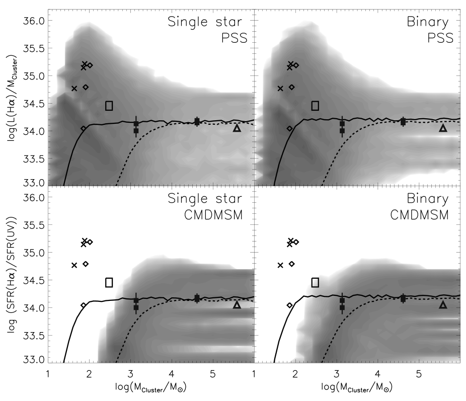
Figure 1: H$\alpha$ flux per $M_{\odot}$ for our synthetic clusters. The shaded contours represent the density of individual realisations of different clusters for two methods of filling the IMF: PSS for upper panels and CMDMSM for the lower panels. The lines show the mean fluxes from these two methods, the solid black line for PSS and dashed black line for CMDMSM. The lines are shown in both single star panels and both binary star panels. The black boxes represent the observations of Calzetti et al. (2010), the lower points include clusters not detected in H$\alpha$ and the high flux value does not include them. The black open box represents the range of possible values derived from the Velorum cluster estimated from Jefferies et al. (2009) and De Marco et al. (2000). The diamonds and crosses are based on data of Lamb et al. (2010). The diamonds represent clusters with upper limits to their mass and the crosses with measured cluster masses. The grey triangle indicates the position of the massive HII region NGC604 with values from Eldridge & Relaño (2011). The left panels are for single-star populations and and the right panels are for binary populations. The linear features in the contours in the panels are due to the limited resolution of the stellar models initial masses and time bins used in the synthesis.

3 Results

3.1 The H$\alpha$ from individual clusters

Calzetti et al. (2010) suggested a novel test for determining how the IMF defines the population of stellar clusters. They studied the production of ionising photons by young clusters in NGC5194. If an IMF is populated purely stochastically then one $10^{5}M_{\odot}$ cluster should have the same stellar content as a hundred $1000M_{\odot}$ clusters. Therefore both samples would have the same H$\alpha$ flux per $M_{\odot}$ of stars. However if the IMF of a $1000M_{\odot}$ cluster is devoid of massive stars due to a link between $M_{\rm max}$ and $M_{\rm Cl}$ then the hundred $1000M_{\odot}$ clusters would have less H$\alpha$ flux per $M_{\odot}$ than a $10^{5}M_{\odot}$ cluster.

For our population of synthetic clusters we have calculated the mean H$\alpha$ flux per $M_{\odot}$ as for the observed clusters of Calzetti et al. (2010). Figure 1 shows our synthetic clusters as points along with the mean H$\alpha$ flux. We see that at cluster masses below $10^{4}M_{\odot}$ the results diverge. With PSS it is possible to have one massive star making up most of the mass of a cluster while with CMDMSM this is not possible. Therefore for PSS and CMDMSM the observed mean H$\alpha$ flux drops from the mean value of around $10^{34.1}{\rm erg\,s^{-1}M_{\odot}^{-1}}$ at around $10^{2}$ or $10^{4}M_{\odot}$ respectively. Therefore by measuring the H$\alpha$ flux for clusters in between these key masses we should be able to determine how nature fills the IMF.

Calzetti et al. (2010) provide two observed values for their two mass bins. The first and higher value does not include clusters that are undetected in H$\alpha$. The second includes these non-detections. The observations at a cluster mass of $10^{4.5}M_{\odot}$ agree with the predicted mean $H\alpha$ flux. However the observed points at $10^{3}M_{\odot}$ are less conclusive. The point without the non-detections lies on the the PSS line, while the point including the non-detections lies in between the PSS and CMDMSM lines. Thus PSS gives a better fit but a refined CMDMSM scheme that allows a higher maximum mass for a certain cluster mass may match the Calzetti et al. (2010) data.

An alternative method to discriminate between PSS and CMDMSM is to search for individual massive stars that are in low-mass clusters. One example is the Wolf-Rayet star $\gamma$-Velorum, the nearest Wolf-Rayet star to the Sun in the Galaxy. It is a binary system containing stars that were initially 35 and 30$M_{\odot}$ in a cluster with a total mass of between 250 and 350$M_{\odot}$ (De Marco et al., 2000; Jefferies et al., 2009; Eldridge, 2009). We have indicated the location of this cluster in Figure 1. We see that the PSS clusters overlap with the parameters of this cluster. The CMDMSM models for a single star population do not reach this region. The binary CMDMSM models do reach the parameter space for $\gamma$-Velorum. The small number of such models indicates such clusters would be rare. This suggests that PSS is more likely to be in action in nature although a more relaxed form of CMDMSM would also fit the observed data.

Other more extreme examples of low-mass clusters with a single massive star were observed by Lamb et al. (2010). They observed apparently isolated O stars and found low mass clusters associated with these stars. Using the stellar and cluster masses derived by Lamb et al. (2010) and estimating the ionising flux for the massive star we have plotted their clusters in Figure 1. They are only reproduced by our PSS method.

This agrees with previous studies by Testi et al. (1997) Testi, Palla & Natta (1998, 1999) and Parker & Goodwin (2007) who use similar arguments. Maschberger & Clarke (2008) also made a detailed study of all available information and also favour PSS. However Weidner, Kroupa & Bonnell (2010) performed a similar analysis and found that for low mass clusters, below $100M_{\odot}$ PSS is favoured but more massive clusters appears to have a CMDMSM relation. The observations of Calzetti et al. (2010) do not currently favour either PSS or CMDMSM. Here we can only agree that PSS occurs in low-mass, up to $100M_{\odot}$, clusters. For more massive clusters, of around $1000M_{\odot}$, it is difficult to differentiate between PSS and CMDMSM. Finally for cluster masses more than about $10^{4}M_{\odot}$ the differences are less important.

Finally we note that our results are in line with those of Villaverde, Cerviño & Luridiana (2010b). They suggest that for cluster masses below $10^{4}M_{\odot}$ there is a highly asymmetric scatter of the ionising flux around the mean integrated values from standard synthesis models because the single most massive star dominates the ionising flux of the cluster. This manifests itself in our results by the increased spread in H$\alpha$ flux per $M_{\odot}$ at low cluster masses. We note that they suggest that PSS is more favoured than CMDMSM.

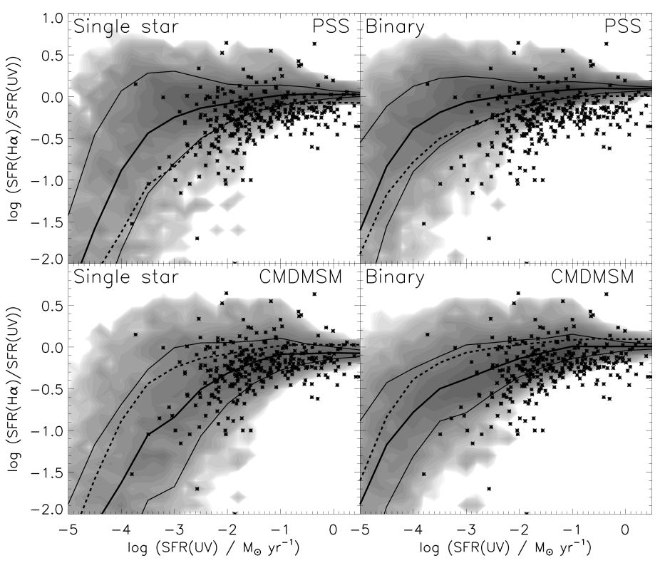
Figure 2: The ratio of SFR measured by H$\alpha$ and UV fluxes verses the SFR from UV flux. The asterisks are the observations of Lee et al. (2009) while the shaded region show the density of our individual realisations of synthetic galaxies. The thick solid lines indicate the mean ratios for the synthetic galaxies and their $1\sigma$ limits. The dashed lines show the mean ratios for the other IMF filling method with the same stellar population. The upper panels are for PSS and the lower panels are for CMDMSM. While the left panels are for a single star population and the right panels are for binary populations. Here we assume that a star formation rate of $1M_{\odot}\,{\rm yr^{-1}}$ is equivalent to a $\log_{10}(F({\rm H}\alpha)/{\rm ergs\,s^{-1}})=41.1$ and a UV flux density of $\log_{10}(F(1500\AA)/{\rm ergs\,s^{-1}\,\AA})=27.85$. Linear features are due to limited resolution in initial mass, separation and mass ratio parameter space of our binary models.

3.2 The H$\alpha$ and FUV in 11HUGS galaxies

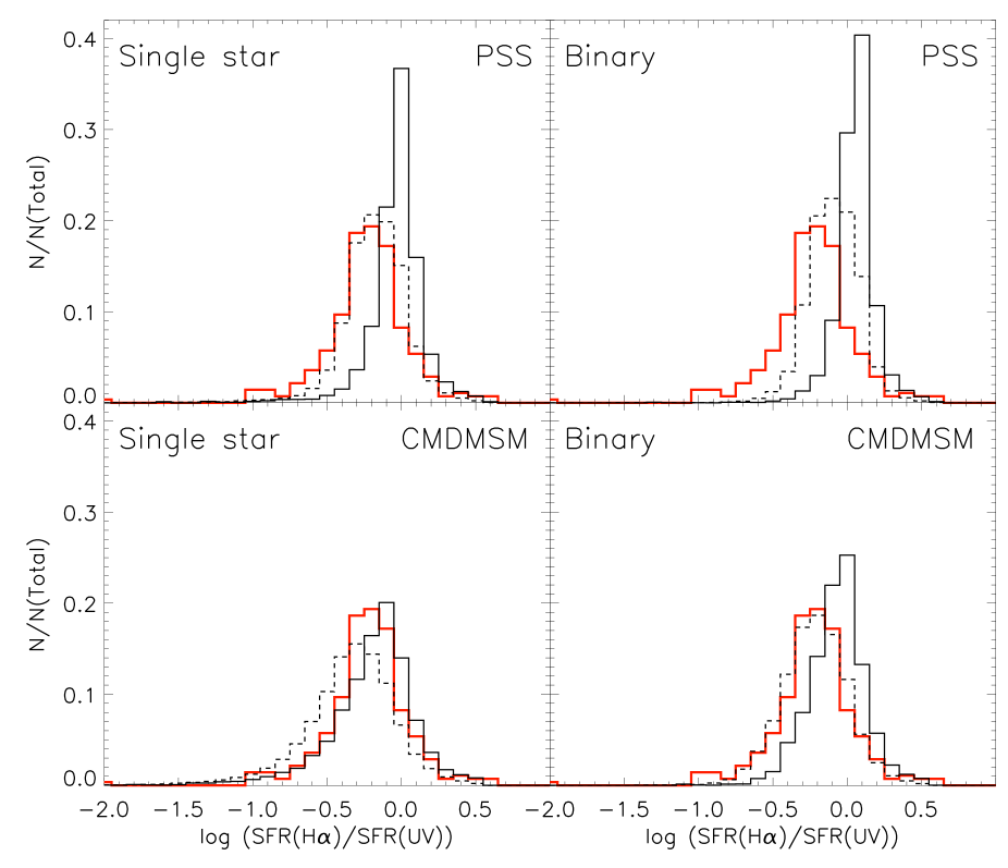
Figure 3: The distribution of H$\alpha$ to UV ratio for observed and synthetic galaxies with star-formation rates between $10^{-2}$ and 1 $M_{\odot}{\rm y^{-1}}$. The red line represents the observed sample of Lee et al. (2009) while the solid line represents the relevant synthetic galaxies from Figure 2. The dashed line represents the synthetic observations smeared by a flat leakage of ionising photons distributed between a leakage fraction of 0 and 50 per cent. The left panels are for PSS and the right panels are for CMDMSM. The first and third panels are for a single star population and the second and fourth panels are for binary populations.

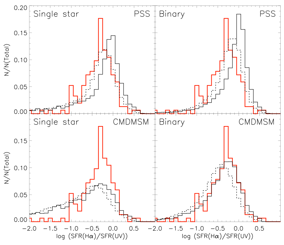
Figure 4: The distribution of H$\alpha$ to UV ratio for observed and synthetic galaxies with star-formation rates between $10^{-4}$ and $10^{-2}$ $M_{\odot}{\rm yr^{-1}}$. The red line represents the observed sample of Lee et al. (2009) while the solid line represents the relevant synthetic galaxies from Figure 2. The dashed line represents the synthetic observations smeared by a flat leakage of ionising photons distribution between a leakage fraction of 0 and 50 per cent. The left panels are for PSS and the right panels are for CMDMSM. While the first and third panels are for a single star population and the second and fourth panels are for binary populations.

Lee et al. (2009), Meurer et al. (2009) and Boselli et al. (2009) have attempted to gain insight into the IMF by looking at emission from entire galaxies. They brought together H$\alpha$ observations with far UV continuum observations. Here we concentrate on the results of Lee et al. (2009) because their set of galaxies are a volume limited sample of 315 within 11 Mpc. The emission of these two spectral star-formation rate indicators are determined by the number of stars with masses greater than 20 and 3$M_{\odot}$ respectively. Therefore measuring the ratio of the two fluxes, or the relative star-formation rates measured for the galaxies, gives an indication of the number of stars in different mass regimes. Lee et al. (2009) found that as the H$\alpha$ flux decreases the H$\alpha$/UV ratio decreases so there is more UV flux than expected. Pflamm-Altenburg, Weidner & Kroupa (2009) have suggested that this turn down is evidence for IGIMF determining the galaxy-wide IMF of these galaxies. Their study was based on single star models alone. Here we repeat their analysis with binary as well as single star models and also our stochastic approach to the star-formation history, with stellar clusters forming independently from one another.

We plot our synthetic galaxies in Figure 2. We see that, at star-formation rates above $10^{-2}M_{\odot}{\rm yr^{-1}}$, the spread of models is similar but CMDMSM gives a slightly greater scatter towards lower values of the H$\alpha$/UV ratio. This can be more easily seen in Figure 3 where we bin the synthetic and observed galaxies with star-formation rates above $10^{-2}M_{\odot}{\rm yr^{-1}}$ by their H$\alpha$/UV ratio. CMDMSM has a greater range of ratios because of the relative lack of massive stars in the total stellar population. We see CMDMSM reproduces the lowest ratios at the highest star-formation rates. PSS produces much higher ratios. However in this model we have assumed no leakage of any ionising photons. This would reduce the contribution from the H$\alpha$ flux by up to around 50 per cent (see Zurita et al., 2002, for example). This would lead to lower ratio values at high star-formation rates for both PSS and CMDMSM.

To account for the leakage or loss of ionising photons from a galaxy or absorption by dust grains we have made a simple adjustment to our models. In Figure 3 we have modified our synthetic ratio distributions by assuming that galaxies lose between 0 and 50 per cent of their ionising photons. We take our synthetic populations and smear them by this range of possible leakage fraction so that the mean leakage is 25 per cent. Even for this modest loss of ionising photons the ratio distribution changes the PSS model to match the range of observed galaxies. At the same time the CMDMSM method has a slightly worse agreement. To test the significance of these differences we have used a $\chi^{2}$ test to compare the observed distributions to the synthetic populations. We find that without leakage only CMDMSM with single stars is a probable match. However with leakage only the CMDMSM single star synthetic population is ruled out.

Fumagalli, da Silva & Krumholz (2011) used a leakage fraction of 5 per cent and stated that their results were not dependent on the amount of leakage. This is because they compared the amount of H$\alpha$ to mean values of H$\alpha$ flux which are less sensitive to leakage than the H$\alpha$/UV flux ratio (see their figure 2). They found that for leakage fractions up to 40 per cent their results were unaffected. This is within the mean leakage of 25 per cent that we apply to our models.

For the single star population the greatest difference between PSS and CMDMSM is seen in the different paths of the mean ratio values versus the star-formation rate determined from the UV flux. CMDMSM decreases much sooner than PSS at around $0.1M_{\odot}{\rm yr^{-1}}$. However there is a large possible range around these mean values in both cases and the difference is only approximately $1\sigma$. When we consider the binary population we see that the difference between the two IMF filling methods is substantially reduced. This is because, while the IMF initially leads to fewer massive stars in the CMDMSM case, binary interactions, such as merging and mass-transfer, increase the number of massive stars relative to a single-star population. If we are to distinguish between PSS and CMDMSM by means of the downturn in this ratio we must repeat the analysis that led to Figure 3 for lower star-formation rates. We show the result for star-formation rates between $10^{-2}$ and $10^{-4}M_{\odot}/{\rm yr^{-1}}$ in Figure 4. By eye PSS provides a better fit to the observed population than CMDMSM. This is because CMDMSM has an extended tail of galaxies towards lower ratios. PSS does not have this tail. However including binary stars in the synthetic galaxies reduces it further in both CMDMSM and PSS. Also the tail might not be present in the observed data owing to selection biases. A $\chi^{2}$ test reveals that both PSS populations are a probable match to the observed distribution. The single-star CMDMSM distribution does not match the observed distribution. However our binary CMDMSM population produces an equally likely fit to the observed data. Our results also show that some ionising photon leakage is required if our PSS models are to match observations.

Lee et al. (2009) noted that their results indicate a downturn in the H$\alpha$ to UV ratio at low star-formation rates. This could be explained by the IGIMF model put forward by Pflamm-Altenburg, Weidner & Kroupa (2009). At first comparison of the synthetic and observed galaxies in Figures 2 and 3 tempts us to agree with this deduction. This is mainly because the spread of the observed galaxies at higher star-formation rates is better reproduced by the CMDMSM, single star models. The most significant difference between PSS and CMDMSM is in the region where the star formation rates drop below $10^{-2}M_{\odot}{\rm yr^{-1}}$. All our models are able to reproduce the observed galaxies with the lowest ratios at low star-formation rates. Therefore it is not possible to differentiate between PSS and CMDMSM from these observations. Furthermore the inclusion of binaries in stellar population models means that any difference between PSS and CMDMSM is only apparent at star-formation rates below those in the observed sample of Lee et al. (2009). Therefore, from the observed distribution of H$\alpha$ to FUV ratio, it is not possible to discriminate between PSS and CMDMSM owing to the uncertainties in the importance of binary evolution and ionising photon leakage.

Our conclusions are broadly in line with those of Fumagalli, da Silva & Krumholz (2011). However they compared PSS models to IGIMF models. The IGIMF models restrict the number of massive stars in the synthetic galaxies further because they impose a maximum cluster mass that depends on the total star-formation rate. We have only imposed a cluster mass that dependent maximum stellar mass and have shown that a CMDMSM alone cannot be ruled out.

An important conclusion to draw from our models (and those of Fumagalli, da Silva & Krumholz, 2011; Weisz et al., 2012) is that the scatter and variation of the H$\alpha$/UV ratio is not due to the IMF filling method but it depends more on the star-formation history of each individual galaxy. A general trend we find is that those systems with less star-formation in the last 10 Myr have lower ratios, while those with most of the star formation in the last 10 Myr have higher ratios even at low mean star-formation rates. This is because the stars responsible for H$\alpha$ emission typically have ages of 10 Myr or less. This indicates that any simulation that predicts the properties of a sample of galaxies must take into account the stochastic nature of star-formation and recognise not only that each cluster has its own stellar content but also that each cluster has its own age independent of the other clusters. If there are enough clusters in a galaxy this leads to an average stellar population. However if there are only a few clusters the appearance of the galaxy-wide stellar population can be very different from what might be expected for a simple stellar population with a smooth star-formation history.

3.3 The importance of binaries

From our results it is possible to qualitatively demonstrate the need to use binary star models. For individual clusters binaries seem to have little affect. This is because of the short period of 8 Myr we have used to match the observed clusters in this case. In our synthetic galaxies, with 100 Myr of star-formation, we see that the scatter of the synthetic galaxies is reduced slightly if binaries are included and the mean SFR ratio starts to decrease at lower SFRs. This is more clearly shown in Figure 5 in which we compare populations with different IMFs and single-star to binary star ratios. We see that for a single-star population the ratio begins to drop between $10^{-2}$ and $10^{-3}{\rm M_{\odot}\,yr^{-1}}$ while for binary populations this drop begins between $10^{-3}$ and $10^{-4}{\rm M_{\odot}\,yr^{-1}}$. The binary effect makes it difficult to distinguish between the PSS and CMDMSM IMF filling methods at any star-formation rate.

Binary evolution affects the observed SFRs because through mass transfer between and merging of stars it increases the number of massive stars at the expense of lower-mass stars. We demonstrate this in Figure 5. We see here that binary populations typically produce similar H$\alpha$/UV flux ratios to a single star population when the IMF slope is shallower. That is until low star-formation rates at which point, for a single cluster with a significant population of binary stars we can also expect the apparent IMF to be flatter. Furthermore the most massive star in a cluster might not have been the most massive star when it formed. Therefore interacting binary stars have a strong effect and must be included when attempts are made to determine the IMF from observations of stellar systems.

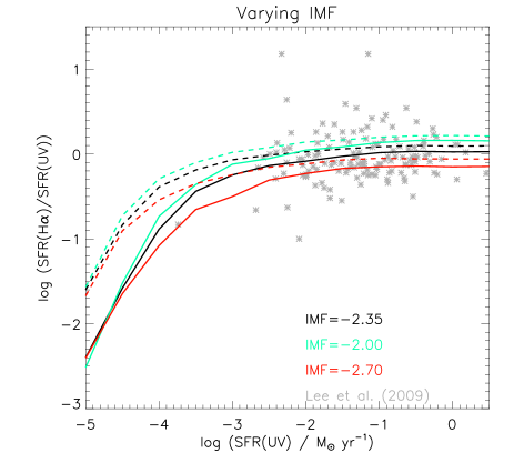
Figure 5: Similar to Figure 2 but here showing the mean ratios for single star (solid lines) and binary star (dashed lines) populations calculated for PSS with different slopes for the SIMF.

4 Conclusions

We have investigated two uncertainties in population synthesis. These are how the IMF is filled and the effects of interacting binary star evolution. The H$\alpha$ flux per $M_{\odot}$ observed in samples of clusters is consistent with PSS of the SIMF for clusters around $100M_{\odot}$ because individual low-mass clusters with one or two massive OB and WR stars, such as the Velorum cluster or those presented by Lamb et al. (2010), provide a strict test to distinguish between PSS and CMDMSM. For more massive clusters comparison with the observations of Calzetti et al. (2010) is not significant enough to rule out CMDMSM. At these masses, around $10^{3}M_{\odot}$ and above, it also becomes more difficult to to differentiate between PSS and CMDMSM because of the blurring effect of binary stars and in addition to the lack of conclusive data in this mass range.

We have also considered the ratio of the H$\alpha$ to UV fluxes in galaxies. Observationally there is a significant scatter that can be explained by the stochastic nature of the star-formation history. We find it difficult to differentiate between PSS and CMDMSM. This is because we find some evidence that the leakage or loss of ionising photons must be considered. In addition, including binary star populations makes it difficult to distinguish between the methods for filling the IMF. Only single-star CMDMSM populations can be ruled out with the observations of galaxies with SFRs below $10^{-2}M_{\odot}{\rm yr^{-1}}$.

The ratio of H$\alpha$ to UV flux for stellar populations, including binary stars, varies less than that for populations of single stars. Binaries can merge and mass-transfer can produce more massive stars than were present in the initial population. Therefore the expected star-formation rates for galaxies in which it will be possible to detect differences between PSS and CMDMSM are much lower than currently observed. Furthermore, because the leakage or loss of ionising photons from young stellar populations must be considered, it becomes even more difficult to discern the IMF-filling method from observations of galaxies with low H$\alpha$ to UV ratios. We suggest that it may be more fruitful to find galaxies with low overall star-formation rates but with high H$\alpha$ to UV ratios. That is galaxies that are rich in clusters similar to those found by Lamb et al. (2010).

5 Acknowledgements

JJE would like to thank the anonymous referee for his very constructive comments which have lead to a much improved paper. JJE is supported by the Institute of Astronomy’s STFC Theory Rolling grant. JJE would also like to thank Joe Walmswell, Monica Relano, Ben Johnson, Dan Weisz, Janice Lee, Daniella Calzetti, Sally Oey, Mark Gieles, Mieguel Cerviño, Michele Fumagalli, Robert da Silva and Christopher Tout for very helpful discussions and comments on this paper.

References

- Bastian, Covey & Meyer (2010) Bastian N., Covey K.R., Meyer M.R., 2010, ARA&A, 48, 339B
- Boselli et al. (2009) Boselli A., Boissier S., Cortese L., Buat V., Hughes T.M., Gavazzi G., 2009, ApJ, 706, 1527B
- Bouy et al. (2003) Bouy H., Brandner W., Mart n E.L., Delfosse X., Allard F., Basri G., 2003, AJ, 126, 1526B
- Bressert et al. (2010) Bressert E., et al., 2010, MNRAS, 409L, 54B
- Calzetti et al. (2010) Calzetti D., Chandar R., Lee J. C., Elmegreen B. G., Kennicutt R. C., Whitmore, B., 2010, ApJ, 719L, 158C
- Cerviño et al (2003) Cerviño M., Luridiana V., P rez E., V lchez J.M., Valls-Gabaud, D., 2003, A&A, 407, 177C
- Chabrier (2003) Chabrier G., 2003, PASP, 115, 763C
- De Marco et al. (2000) De Marco O., Schmutz W., Crowther P. A., Hillier D. J., Dessart L., de Koter A., Schweickhardt J. 2000, A&A, 358, 187
- Duquennoy & Mayor (1991) Duquennoy A., Mayor M., 1991, A&A, 248, 485D
- Eldridge, Izzard & Tout (2008) Eldridge J.J., Izzard R.G., Tout C.A., 2008, MNRAS, 384, 1109E
- Eldridge (2009) Eldridge J.J., 2009, MNRAS, 400, L20
- Eldridge & Stanway (2009) Eldridge J.J., Stanway E.R. 2009, MNRAS, 400, 1019E
- Eldridge & Relaño (2011) Eldridge J.J., Relaño M., MNRAS, 411, 235E
- Eldridge, Langer & Tout (2011) Eldridge J.J., Langer N., Tout C.A., 2011, MNRAS in press
- Elmegreen (2006) Elmegreen B.G., 2006, ApJ, 648, 572E
- Fregeau, Ivanova & Rasio (2009) Fregeau J.M., Ivanova N., Rasio F.A., 2009, ApJ, 707, 1533F