Residual Component Analysis

Abstract

Probabilistic principal component analysis (PPCA) seeks a low dimensional representation of a data set in the presence of independent spherical Gaussian noise, $\mathbf{\Sigma}=\sigma^{2}\mathbf{I}$. The maximum likelihood solution for the model is an eigenvalue problem on the sample covariance matrix. In this paper we consider the situation where the data variance is already partially explained by other factors, e.g. covariates of interest, or temporal correlations leaving some residual variance. We decompose the residual variance into its components through a generalized eigenvalue problem, which we call residual component analysis (RCA). We show that canonical covariates analysis (CCA) is a special case of our algorithm and explore a range of new algorithms that arise from the framework. We illustrate the ideas on a gene expression time series data set and the recovery of human pose from silhouette.

1 Introduction

Probabilistic principal component analysis (PPCA) decomposes the covariance of a data point, $\mathbf{y}$, into a low rank term and a diagonal noise term. The underlying probabilistic model assumes that each datum is Gaussian distributed,

$$\mathbf{y}\sim\mathcal{N}(\mathbf{0},\mathbf{W}\mathbf{W}^{\top}+\sigma^{2}\mathbf{I}),$$

where we assume the data is centred such that its mean is zero and $\mathbf{W}\in\Re^{d\times q}$ imposes a reduced rank structure on the covariance ($q<d-1$). The log likelihood of the centered data set with $n$ data points, $\mathbf{Y}\in\Re^{n\times d}$,

$$\log p(\mathbf{Y})=\sum_{i=1}^{n}\log\mathcal{N}(\mathbf{y}_{i,:}|\mathbf{0},\mathbf{W}\mathbf{W}^{\top}+\sigma^{2}\mathbf{I}),$$

can be maximized (Tipping and Bishop, 1999) with the result that $\mathbf{W}=\mathbf{U}_{q}\mathbf{L}_{q}\mathbf{R}^{\top}$, where $\mathbf{U}_{q}$ are the $q$ principal eigenvectors of the sample covariance, $\mathbf{S}=n^{-1}\mathbf{Y}^{\top}\mathbf{Y}$, $\mathbf{L}_{q}$ is a diagonal matrix with elements $\ell_{i,i}=\sqrt{\lambda_{i}-\sigma^{2}_{n}}$, where $\lambda_{i}$ is the $i$th eigenvalue of the sample covariance, $\mathbf{R}$ is an arbitrary rotation matrix, and $\sigma^{2}_{n}$ the noise variance. As a result the matrix $\mathbf{W}$ spans the principal subspace of the data and the model is known as principal components analysis. Underlying this model is an assumption that the data set can be represented by

$$\mathbf{Y}=\mathbf{X}\mathbf{W}^{\top}+\mathbf{E}$$

where $\mathbf{X}\in\Re^{n\times q}$ is the matrix of $q$-dimensional latent variables and $\mathbf{E}$ is a matrix of noise variables, each element being independently sampled from a zero mean Gaussian with variance $\sigma^{2}$. The marginal likelihood above is obtained by placing an isotropic prior independently on the elements of $\mathbf{X}$, $x_{i,j}\sim\mathcal{N}(0,1)$.

Lawrence (Lawrence, 2005) showed that the PCA solution is also obtained for log likelihoods of the form

$$\log p(\mathbf{Y})=\sum_{j=1}^{d}\log\mathcal{N}(\mathbf{y}_{:,j}|\mathbf{0},\mathbf{X}\mathbf{X}^{\top}+\sigma^{2}\mathbf{I})$$

which is recovered when we marginalize $\mathbf{W}$ with an isotropic prior instead of $\mathbf{X}$. This is a dual form of probabilistic PCA which could also be called probabilistic principal coordinate analysis as the maximum likelihood solution solves for the latent coordinates, $\mathbf{X}=\mathbf{U}^{\prime}_{q}\mathbf{L}\mathbf{R}^{\top}$, instead of the principal subspace. Here $\mathbf{U}^{\prime}_{q}$ are the first $q$ principal eigenvectors of the inner product matrix $\mathbf{Y}\mathbf{Y}^{\top}$ with $\mathbf{L}$ defined as before. Note in this case that the Gaussian density is independent across data features rather than data points. So the correlation is expressed between data points. The underlying model is in fact an product of independent Gaussian processes (Rasmussen and Williams, 2006) with linear covariance functions.

Both of these scenarios involve maximizing log likelihoods of a similar structure, namely the covariance of the Gaussians is given by a low rank term plus a spherical term, $\mathbf{X}\mathbf{X}^{\top}+\sigma^{2}\mathbf{I}$ (dual scenario). In this paper we consider an alternative form where the covariance is given by $\mathbf{X}\mathbf{X}^{\top}+\mathbf{\Sigma}$, where $\mathbf{\Sigma}$ is a general positive definite matrix. Our motivation is that our data has already been partly explained by the covariance matrix $\mathbf{\Sigma}$ and we wish to study the components of the residuals. Our ideas can be applied in both the primal and dual representations: the form to be used depends on what information we wish to include in $\mathbf{\Sigma}$.

As a motivating example consider a linear additive model (Figure 1),

$$\mathbf{Y}=\mathbf{X}\mathbf{W}^{\top}+\mathbf{Z}\mathbf{V}^{\top}+\mathbf{E},$$ (1)

where $\mathbf{Z}$ is a matrix of known covariates that are assumed to have some predictive power for $\mathbf{Y}$ and $\mathbf{X}$ is a matrix of unknown confounders (as in standard PPCA). Also consider that $\mathbf{Y}$ could be a set of $n$ patients’ gene expression measurements ($d$ genes), $\mathbf{Z}$ could be the genotype of each patient and $\mathbf{X}$ could be unobserved environmental confounders (see (Author, )). We can marginalize out $\mathbf{V}$ with a Gaussian prior, $v_{i,j}\sim\mathcal{N}(0,\alpha)$ as well as $\mathbf{W}$ with a prior $w_{i,j}\sim\mathcal{N}(0,1)$ and recover

$$\log p(\mathbf{Y})=\sum_{j=1}^{d}\log\mathcal{N}(\mathbf{y}_{:,j}|\mathbf{0},\mathbf{X}\mathbf{X}^{\top}+\mathbf{\Sigma}),$$

where for this example $\mathbf{\Sigma}=\alpha\mathbf{Z}\mathbf{Z}^{\top}+\sigma^{2}\mathbf{I}$.

Given $\mathbf{\Sigma}$, can we solve for $\mathbf{X}$? As we will show, the solution for $\mathbf{X}$ is given by a generalized eigenvalue problem. By using different forms for $\mathbf{\Sigma}$ we can formulate different models. For example, for a particular choice of $\mathbf{\Sigma}$ we recover canonical correlates analysis (CCA, see Section 2.1). In the next section we show how the low rank term can be optimized for general $\mathbf{\Sigma}$. The only constraints that we place on $\mathbf{\Sigma}$ are that it should be positive definite and invertible.

2 Optimizing the Likelihood

The log likelihood for the RCA model is given by

$$L(\mathbf{X},\mathbf{\Sigma})=-\frac{d}{2}\ln\left|{\mathbf{K}}\right|-\frac{1}{2}\mathrm{tr}({\mathbf{Y}\mathbf{Y}^{\top}\mathbf{K}^{-1}})-\frac{nd}{2}\ln(2\pi),$$ (2)

where we have defined $\mathbf{K}\equiv\mathbf{X}\mathbf{X}^{\top}+\mathbf{\Sigma}$. We now take the eigendecomposition of $\mathbf{\Sigma}$,

$$\mathbf{\Sigma}=\mathbf{U}\mathbf{\Lambda}\mathbf{U}^{\top},$$ (3)

where $\mathbf{U}^{\top}\mathbf{U}=\mathbf{I}$ and $\mathbf{\Lambda}$ is a diagonal matrix. We now project the covariance onto this eigenbasis scaling with the eigenvalues,

$$\hat{\mathbf{K}}=\mathbf{\Lambda}^{-\frac{1}{2}}\mathbf{U}^{\top}\mathbf{K}\mathbf{U\Lambda}^{-\frac{1}{2}}=\mathbf{\Lambda}^{-\frac{1}{2}}\mathbf{U}^{\top}\mathbf{X}\mathbf{X}^{\top}\mathbf{U\Lambda}^{-\frac{1}{2}}+\mathbf{I}.$$ (4)

This allows us to define

$$\hat{\mathbf{K}}\equiv\hat{\mathbf{X}}\hat{\mathbf{X}}^{\top}+\mathbf{I},\quad\textrm{where}\quad\hat{\mathbf{X}}\equiv\mathbf{\Lambda}^{-\frac{1}{2}}\mathbf{U}^{\top}\mathbf{X},$$ (5)

and also implies the inverse

$$\hat{\mathbf{K}}^{-1}=\mathbf{\Lambda}^{\frac{1}{2}}\mathbf{U}^{\top}\mathbf{K}^{-1}\mathbf{U\Lambda}^{\frac{1}{2}}.$$ (6)

Now we note from eq. (4) that

$$\left|{\mathbf{K}}\right|=\hat{\left|\mathbf{K}\right|}\left|\mathbf{\Lambda}\right|,$$

and from eq. (6) that

$$\mathrm{tr}(\mathbf{Y}\mathbf{Y}^{\top}\mathbf{K}^{-1})=\mathrm{tr}(\mathbf{\Lambda}^{-\frac{1}{2}}\mathbf{U}^{\top}\mathbf{Y}\mathbf{Y}^{\top}\mathbf{U}\mathbf{\Lambda}^{-\frac{1}{2}}\hat{\mathbf{K}}^{-1}),$$

leading us to define $\hat{\mathbf{Y}}\equiv\mathbf{\Lambda}^{-\frac{1}{2}}\mathbf{U}^{\top}\mathbf{Y}$ so that we can rewrite the entire likelihood from eq. (2) as

$$L(\mathbf{X},\mathbf{\Lambda},\mathbf{U})=-\sum_{i=1}^{n}d\ln\lambda_{i}-\frac{d}{2}\ln\hat{\left|\mathbf{K}\right|}-\frac{1}{2}\mathrm{tr}(\mathbf{\hat{Y}}\mathbf{\hat{Y}^{\top}}\hat{\mathbf{K}}^{-1})-\frac{nd}{2}\ln(2\pi).$$

We know how to maximize this new likelihood with respect to $\hat{\mathbf{X}}$. Following a similar route to the maximum likelihood solution proof in (Tipping and Bishop, 1999), we take the gradient of the likelihood with respect to $\mathbf{\hat{X}}$

$$\begin{split}&\frac{\partial L}{\partial\hat{\mathbf{X}}}=\hat{\mathbf{K}}^{-1}\hat{\mathbf{Y}}\hat{\mathbf{Y}}^{\top}\hat{\mathbf{K}}^{-1}\hat{\mathbf{X}}-\hat{\mathbf{K}}^{-1}\hat{\mathbf{X}}=\mathbf{0},\quad\textrm{to give the stationary point}\quad\hat{\mathbf{Y}}\hat{\mathbf{Y}}^{\top}\hat{\mathbf{K}}^{-1}\hat{\mathbf{X}}=\hat{\mathbf{X}}.\end{split}$$ (7)

By singular value decomposition on $\hat{\mathbf{X}}$, we get

$$\hat{\mathbf{X}}=\hat{\mathbf{V}}\mathbf{L}\mathbf{R}^{\top},$$ (8)

then by substituting $\mathbf{\hat{X}}$ in eq. (7) and eq. (5)

$$\begin{split}\hat{\mathbf{V}}\mathbf{L}\mathbf{R}^{\top}&=\hat{\mathbf{Y}}\hat{\mathbf{Y}}^{\top}(\hat{\mathbf{V}}\mathbf{L}^{2}\hat{\mathbf{V}}^{\top}+\mathbf{I})^{-1}\hat{\mathbf{V}}\mathbf{L}\mathbf{R}^{\top}\\ \hat{\mathbf{V}}(\mathbf{L}^{2}+\mathbf{I})&=\hat{\mathbf{Y}}\hat{\mathbf{Y}}^{\top}\hat{\mathbf{V}},\end{split}$$

where we make use of the Woodbury matrix indentity. Now we see that maximisation relies on a regular eigenvalue problem of the form

$$\begin{split}\hat{\mathbf{Y}}\hat{\mathbf{Y}}^{\top}\hat{\mathbf{V}}&=\hat{\mathbf{V}}\mathbf{D},\quad\textrm{where}\\ \mathbf{D}&\equiv(\mathbf{L}^{2}+\mathbf{I}).\end{split}$$ (9)

We now express this eigenvalue problem in terms of $\mathbf{Y}\mathbf{Y}^{\top}$. Substituting $\mathbf{X}=\mathbf{U\Lambda}^{\frac{1}{2}}\hat{\mathbf{X}}$ and by eq. (8), we get a decomposition of $\mathbf{X}$ with the same singular values as $\mathbf{\hat{X}}$

$$\mathbf{X}=\mathbf{U\Lambda}^{\frac{1}{2}}\hat{\mathbf{V}}\mathbf{L}\mathbf{R}^{\top}=\mathbf{T}\mathbf{L}\mathbf{R}^{\top},$$ (10)

where we have defined $\hat{\mathbf{V}}\equiv\mathbf{\Lambda}^{-\frac{1}{2}}\mathbf{U^{\top}T}$. Substituting for $\mathbf{\hat{Y}}$ and $\mathbf{\hat{V}}$ in the eigenvalue problem from eq. (9), recovers the eigenvalue problem in the original dual-space

$$\begin{split}\mathbf{\Lambda}^{-\frac{1}{2}}\mathbf{U}^{\top}\mathbf{Y}\mathbf{Y}^{\top}\mathbf{U\Lambda}^{-1}\mathbf{U}^{\top}\mathbf{T}&=\mathbf{\Lambda}^{-\frac{1}{2}}\mathbf{U}^{\top}\mathbf{T}\mathbf{D}\\ \mathbf{Y}\mathbf{Y}^{\top}\mathbf{\Sigma}^{-1}\mathbf{T}&=\mathbf{T}\mathbf{D},\end{split}$$

which follows from the inverse of eq. (3).

So far, $\mathbf{T}$ is solved via a non-symmetric eigenvalue problem. Assuming that $\mathbf{\Sigma}$ is positive-definite (i.e. invertible), we define $\mathbf{S}\equiv\mathbf{\Sigma}^{-1}\mathbf{T}$ and get

$$\mathbf{Y}\mathbf{Y}^{\top}\mathbf{S}=\mathbf{\Sigma}\mathbf{S}\mathbf{D}$$

which is in the desired form of a generalized eigenvalue problem. Now we can recover $\mathbf{X}$, up to rotation ($\mathbf{R=I}$), via the first $q$ generalised eigenvectors of $\mathbf{Y}\mathbf{Y}^{\top}$ and eq. (10)

$$\mathbf{X}=\mathbf{T}\mathbf{L}=\mathbf{\Sigma}\mathbf{S}\mathbf{L}=\mathbf{\mathbf{\Sigma}}\mathbf{S}\mathbf{(D-I)}^{\frac{1}{2}}.$$

Due to the algebraic symmetry between our dual and primal formulations of the log-marginal likelihood, we can easily extend our derivations to the primal representation. For example, in the linear model in eq. (1)), the maximum likelihood solution of $\mathbf{W}$ is computed through

$$\mathbf{Y^{\top}}\mathbf{Y}\mathbf{S}=\mathbf{\Sigma}\mathbf{S}\mathbf{D},\quad\textrm{where}\quad\mathbf{\Sigma}=\alpha\mathbf{V}\mathbf{V}^{\top}+\sigma^{2}\mathbf{I}\quad\textrm{and}\quad\mathbf{W}=\mathbf{\Sigma}\mathbf{S}\mathbf{(D-I)}^{\frac{1}{2}}.$$ (11)

2.1 Equivalence to CCA

Canonical covariates analysis is solved through a generalized eigenvalue problem (De Bie et al., 2005; Bach and Jordan, 2002).

$$\begin{pmatrix}\mathbf{0}&\mathbf{C}_{12}\\ \mathbf{C}_{12}^{\top}&\mathbf{0}\end{pmatrix}\begin{pmatrix}\mathbf{S}_{1}\\ \mathbf{S}_{2}\end{pmatrix}=\begin{pmatrix}\mathbf{C_{11}}&\mathbf{0}\\ \mathbf{0}&\mathbf{C}_{22}\end{pmatrix}\begin{pmatrix}\mathbf{S}_{1}\\ \mathbf{S}_{2}\end{pmatrix}\mathbf{\Lambda},$$

which can be rewritten as

$$\begin{pmatrix}\mathbf{C}_{11}&\mathbf{C}_{12}\\ \mathbf{C}_{12}^{\top}&\mathbf{C}_{22}\end{pmatrix}\begin{pmatrix}\mathbf{S}_{1}\\ \mathbf{S}_{2}\end{pmatrix}=\begin{pmatrix}\mathbf{C}_{11}&\mathbf{0}\\ \mathbf{0}&\mathbf{C}_{22}\end{pmatrix}\begin{pmatrix}\mathbf{S}_{1}\\ \mathbf{S}_{2}\end{pmatrix}(\mathbf{\Lambda+I}).$$

A few notes on CCA: The left-most block matrix is the sample covariance matrix of the joint (augmented) design matrix $\mathbf{C}=n^{-1}(\mathbf{Y}_{1},\mathbf{Y}_{2})^{\top}(\mathbf{Y}_{1},\mathbf{Y}_{2})\quad\textrm{and}\quad\mathbf{C}_{11}=n^{-1}\mathbf{Y}_{1}^{\top}\mathbf{Y}_{1},\quad\mathbf{C}_{22}=n^{-1}\mathbf{Y}_{2}^{\top}\mathbf{Y}_{2},\quad\mathbf{C}_{12}=n^{-1}\mathbf{Y}_{1}^{\top}\mathbf{Y}_{2}$ are the individual sample covariances and cross-covariance of $\mathbf{Y}_{1},\mathbf{Y}_{2}$. The diagonal matrix of generalised eigenvalues, $\mathbf{\Lambda}$, contains the canonical correlations. The generalised eigenvectors, made up of direction-pairs $\mathbf{S}_{1},\mathbf{S}_{2}$, are the canonical-directions or coefficients in data-spaces $\mathcal{Y}_{1},\mathcal{Y}_{2}$ respectively. They maximise the correlation between a projection $\mathbf{Y}_{1}\mathbf{S}_{1}$ of features of $\mathbf{Y}_{1}$ and a projection $\mathbf{Y}_{2}\mathbf{S}_{2}$ of features of $\mathbf{Y}_{2}$,

$$\mathbf{S}_{1}^{\top}\mathbf{C}_{12}\mathbf{S}_{2}=\mathbf{P},\quad\textrm{such that}\quad\mathbf{S}_{1}^{\top}\mathbf{C}_{11}\mathbf{S}_{1}=\mathbf{S}_{2}^{\top}\mathbf{C}_{22}\mathbf{S}_{2}=\mathbf{I},$$

where $\mathbf{P}$ is a rectangular matrix with the canonical correlations on its diagonal. These projections are known as the canonical variates.

To show the equivalence of RCA to CCA, we turn our attention to the generalised eigenvalue problem of RCA in eq. (11) and consider the case where

$$\mathbf{\Sigma}=\begin{pmatrix}\mathbf{Y}_{1}^{\top}\mathbf{Y}_{1}&\mathbf{0}\\ \mathbf{0}&\mathbf{Y}_{2}^{\top}\mathbf{Y}_{2}\end{pmatrix}.$$

Then by inspection, the generalised eigenvectors $\mathbf{S}$ of RCA become the canonical directions and $(\mathbf{D-I})$ becomes the diagonal matrix of canonical correlations. (Bach and Jordan, 2005) showed that the CCA maximum likelihood solutions for $\mathbf{V}_{1},\mathbf{V}_{2}$ in the graphical model of Figure 1 (again, for centred $\mathbf{y}_{1},\mathbf{y}_{2}$)

$$\begin{pmatrix}\mathbf{y}_{1}\\ \mathbf{y}_{2}\end{pmatrix}\sim\mathcal{N}\left(\begin{pmatrix}\mathbf{V}_{1}\\ \mathbf{V}_{2}\end{pmatrix}\mathbf{z},\begin{pmatrix}\bm{\epsilon}_{1}&\mathbf{0}\\ \mathbf{0}&\bm{\epsilon}_{2}\end{pmatrix}\right),$$

are $\mathbf{V}_{1}=\mathbf{C}_{11}\mathbf{S}_{1}^{(q)}\mathbf{\Lambda}^{1/2}_{q}\mathbf{R}$ and $\mathbf{V}_{2}=\mathbf{C}_{22}\mathbf{S}_{2}^{(q)}\mathbf{\Lambda}^{1/2}_{q}\mathbf{R}$, where $\bm{\epsilon}_{1}$ and $\bm{\epsilon}_{2}$ are full noise covariance matrices, $\mathbf{S}_{1}^{(q)}$ and $\mathbf{S}_{2}^{(q)}$ are the first $q$ canonical directions, $\bm{\Lambda}_{q}$ is the diagonal matrix of the first $q$ canonical correlations and the arbitrary rotations $\mathbf{R}=\mathbf{I}$. These maximum likelihood solutions are equivalent to $\mathbf{W}$ in eq. (11), when $\mathbf{\Sigma}=\mathbf{C}_{11}$, $\mathbf{S}=\mathbf{S}_{1}^{(q)}$ for $\mathbf{V}_{1}$ and $\mathbf{\Sigma}=\mathbf{C}_{22}$, $\mathbf{S}=\mathbf{S}_{2}^{(q)}$ for $\mathbf{V}_{2}$.

Similarly, we get the PCA eigenvalue equation when $\mathbf{\Sigma}=\mathbf{I}$ and the PPCA solution emerges as

$$\mathbf{W}=\mathbf{S}\mathbf{(D-I)}^{\frac{1}{2}}=\mathbf{U}_{q}(\mathbf{\Lambda}_{q}-\mathbf{I})^{\frac{1}{2}}.$$

We notice a subtle difference from the PPCA formulation here. Whereas PPCA explicitly subtracts the noise variance from the $q$ retained principal eigenvalues, RCA already incorporates any noise terms in $\mathbf{\Sigma}$ and standardises them while projecting the total covariance onto the eigenbasis of $\mathbf{\Sigma}$, see eq. (4).

From the RCA perspective, CCA can be seen as setting $\mathbf{\Sigma}$ to be block diagonal, with each block containing the sample covariance matrix associated with the data. The residual components then represent the variance which isn’t explained by those two sample covariances: i.e. the correlation between the two data sets. Residual components analysis is much general than this though, by alternative choices for $\mathbf{\Sigma}$ we can explore other residual components. To demonstrate this we now consider two case study data sets. The first is a gene expression experiment containing treatment and control, our objective will be to explore the differences between treatment and control. The second is a data set of human pose and silhouette (Agarwal and Triggs, 2006). Our objective is to predict the pose given the silhouette and we find a set of components which we can project the data on to achieve this.

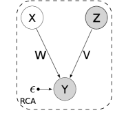
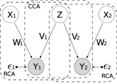
Figure 1: 1 Graphical model of RCA. $\mathbf{Z}$ partially explains the variation in $\mathbf{Y}$ through the sub-space defined in $\mathbf{V}$. The residual covariance is spanned by $\mathbf{W}$ up to some noise variance of $\mathbf{\epsilon}$. 1 Graphical model of PCCA. $\mathbf{Z}$ is latent and shared between $\mathbf{Y}_{1}$ and $\mathbf{Y}_{2}$. The standard linear approach to estimating $\mathbf{V}_{1},\mathbf{V}_{2}$ and $\mathbf{Z}$ is via CCA, which turns out to be a special case of RCA (cf. section 2.1). 1 In a multi-view learning context, $\mathbf{Y}_{1},\mathbf{Y}_{2}$ have shared ($\mathbf{Z}$) and private ($\mathbf{X}_{1}$, $\mathbf{X}_{2}$) latent components. We illustrate an iterative-RCA approach for inference in this type of model.

3 Case Study 1: Differences in Gene Expression Profiles

A common data analysis challenge is to summarize the difference between treatment and control. To illustrate how RCA can help, we consider two gene expression time series of cell lines. The treatment cells are targeted by TP63 introduced into the nucleus by tamoxifen. The control cells are simply subject to tamoxifen alone. The data used for this case study come from (Della Gatta et al., 2008). The treatment group ($\mathbf{Y}_{1}$) contains $n_{1}=13$ time points of $d=22,690$ gene expression measurements, whilst the control group ($\mathbf{Y}_{2}$) contains only $n_{2}=7$ time points. This complexity of data (with different numbers of time points and non-uniform sampling) is typical of many bio-medical data sets. The challenge is to represent the differences between the gene expression profiles for these two data sets. Canonical correlates analysis could be applied but this would represent the similarities between the data not the differences. Our approach is as follows. First we assume that both time series are identical, that would imply that they could be modeled (for example) by a Gaussian process with a temporal covariance function,

$$\begin{pmatrix}\mathbf{y}_{1}\\ \mathbf{y}_{2}\end{pmatrix}\sim\mathcal{N}(\mathbf{0},\mathbf{K})$$

where the matrix of the covariance function, $\mathbf{K}$, is computed as if both $\mathbf{y}_{1}$ and $\mathbf{y}_{2}$ were from the same function. Now, if we study the residual components, they will be forced to explain how the two time series are actually different. In other words we model the data through the dual paradigm with a covariance of the form

$$\tilde{\mathbf{C}}=\mathbf{X}\mathbf{X}^{\top}+\mathbf{K}$$

and solve to find the residual components $\mathbf{X}$. We used a squared exponential covariance (or RBF kernel) for $\mathbf{K}$ whose elements were $k(t_{i},t_{j})=\exp(-0.5\ell^{-2}(t_{i}-t_{j})^{2})$. The parameters of the covariance function could be optimized, but for simplicity we set $\ell=20$ which provided a bandwidth roughly in line with the time point sampling intervals. We also added a small noise term along the diagonal of $\mathbf{K}$ which was set to 1% of the data variance.

We project the profiles onto the eigenbasis of the first $q$ generalised eigenvectors

$$\mathbf{Y}^{\prime}=\mathbf{S}^{(q)\top}\mathbf{Y}$$

and obtain a score of differential expression based on the norms of their projections. The number $q$ of retained principal eigenvectors is decided on the number of corresponding eigenvalues larger than one. Recall in PPCA (cf. page 1) that as the assumed noise variance $\sigma^{2}_{n}$ increases, more eigenvalues become negative and less eigenvectors are retained in the solution of $\mathbf{W}$. On a similar note, RCA standardises any positive-definite noise (cf. eq. (4)), so we always have to test for eigenvalues larger than 1. Here, the assumed noise variance embedded in the kernel drives the effective number of eigenvectors in the projection.

We rank the scores and compare to a noisy ground truth list of binding targets of TP63 from (Della Gatta et al., 2008), giving the ROC performance curve in Figure 2. The baseline method that we compare against is a Bayesian hierarchical model, BATS (Angelini et al., 2007). We notice that RCA outperforms BATS in terms the area under the ROC curve.

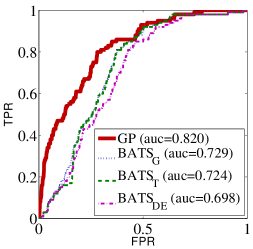
Figure 2: 2 An RBF covariance computed on the augmented time-input vector for the microarray experiment. The covariance is computed across the times for the control and the treatment. $\mathbf{t}=({0:20:240},0,20,40,60,120,180,240)$, with bandwidth parameter $\ell=20$ and noise variance $\sigma^{2}_{n}=10^{-4}$. 2 ROC comparison against BATS, see also Kalaitzis and Lawrence (2011) for details on an alternative approach based on Gaussian processes.

4 Case Study 2: Iterative RCA for Prediction of Pose from Silhouette

Probabilistic canonical correlates analysis explains two related data sets by assuming a full covariance block diagonal form and low rank off diagonal terms. Ek et al.Ek et al. (2008) introduced a model with both a shared latent space and private latent spaces for explaining data specifically associated with the two data sets. The graphical model is shown in Figure 1. Each partition of the data space, $\mathbf{Y}_{1}$ and $\mathbf{Y}_{2}$ has its own associated latent space, $\mathbf{X}_{1}$ and $\mathbf{X}_{2}$ as well as a shared latent space, $\mathbf{Z}$ which corresponds to the standard shared latent space found in CCA. The advantage to a model of this structure is that if the variance that is particular to each partition of the data is low dimensional, this will be recovered. The partitions of the data are therefore modeled as

$$\mathbf{Y}_{1}=\mathbf{X}_{1}\mathbf{W}_{1}^{\top}+\mathbf{Z}\mathbf{V}_{1}^{\top}+\epsilon_{1},\quad\textrm{where}\quad\epsilon_{1}\sim\mathcal{N}(\mathbf{0},\sigma_{1}^{2}\mathbf{I})$$

and

$$\mathbf{Y}_{2}=\mathbf{X}_{2}\mathbf{W}_{2}^{\top}+\mathbf{Z}\mathbf{V}_{2}^{\top}+\epsilon_{2}\quad\textrm{where}\quad\epsilon_{2}\sim\mathcal{N}(\mathbf{0},\sigma_{2}^{2}\mathbf{I}).$$

Each set of latent variables can be marginalized through an isotropic Gaussian prior, $z\sim\mathcal{N}(0,1)$, leading to a covariance structure for the concatenated data set of the following form

$$\tilde{\mathbf{C}}=\begin{pmatrix}\mathbf{W}_{1}\mathbf{W}_{1}^{\top}&\mathbf{0}\\ \mathbf{0}&\mathbf{W}_{2}\mathbf{W}_{2}^{\top}\end{pmatrix}+\begin{pmatrix}\mathbf{V}_{1}\mathbf{V}_{1}^{\top}&\mathbf{V}_{1}\mathbf{V}_{2}^{\top}\\ \mathbf{V}_{2}\mathbf{V}_{1}^{\top}&\mathbf{V}_{2}\mathbf{V}_{2}^{\top}\end{pmatrix}+\begin{pmatrix}\sigma^{2}_{1}\mathbf{I}&\mathbf{0}\\ \mathbf{0}&\sigma^{2}_{2}\mathbf{I}\end{pmatrix}.$$

Setting

$$\mathbf{\Sigma}=\begin{pmatrix}\mathbf{W}_{1}\mathbf{W}_{1}^{\top}&\mathbf{0}\\ \mathbf{0}&\mathbf{W}_{2}{}\mathbf{W}_{2}^{\top}\end{pmatrix}+\begin{pmatrix}\sigma^{2}_{1}\mathbf{I}&\mathbf{0}\\ \mathbf{0}&\sigma^{2}_{2}\mathbf{I}\end{pmatrix}$$

allows $\mathbf{V}_{1}$ and $\mathbf{V}_{2}$ to be optimized using the RCA algorithm. To optimize $\mathbf{W}_{1}$ and $\mathbf{W}_{2}$ we note that the marginal covariance for $\mathbf{Y}_{1}$ is $\tilde{\mathbf{C}}_{11}=\mathbf{W}_{1}\mathbf{W}_{1}^{\top}+\mathbf{V}_{1}\mathbf{V}_{1}^{\top}+\sigma^{2}_{1}\mathbf{I}$, so $\mathbf{W}_{1}$ can be optimized by RCA using $\mathbf{\Sigma}=\mathbf{V}_{1}\mathbf{V}_{1}^{\top}+\sigma^{2}_{1}\mathbf{I}$. A similar optimization can be done for $\mathbf{W}_{2}$.

The data we consider come from Agarwal and Triggs (Agarwal and Triggs, 2006). They produced a set of 3D human poses and associated silhouettes. The silhouettes are summarized by a $d_{2}=100$ dimensional vector of HoG features in matrix $\mathbf{Y}_{2}\in\Re^{n\times d_{2}}$. There are $n=1,927$ frames. There are 21 points in each pose representation each containing $x$, $y$, $z$ coordinates leading to $d_{2}=63$ for $\mathbf{Y}_{1}\in\Re^{n\times d_{1}}$. The data is generated by the Poser computer software, therefore it is “noise free”. To better reflect real world scenarios we added a small amount of Gaussian noise to each feature.

One issue with this iterative RCA algorithm is that 3 latent dimensionalities need to be chosen. However, similar to probabilistic PCA, if the noise values, $\sigma_{1}^{2}$ and $\sigma_{2}^{2}$ are fixed, the latent dimensionality will be determined automatically. We therefore set the noise variances to a proportion, $\alpha$, of the data variance. We used this fraction to control the dimensionality, varying it between 0 and 1. This gave us only one parameter in the model to vary. The algorithm converges when the log-marginal likelihood between two iterations differs no more than a small constant.

Algorithm 1 Iterative RCA

  $\mathbf{C}\leftarrow n^{-1}\mathbf{Y}^{\top}\mathbf{Y},\quad\mathbf{C}_{11}\leftarrow n^{-1}\mathbf{Y}_{1}^{\top}\mathbf{Y}_{1},\quad\mathbf{C}_{22}\leftarrow n^{-1}\mathbf{Y}_{2}^{\top}\mathbf{Y}_{2}$

  Initialize $\alpha\in[0,1],\quad\sigma^{2}_{1}\leftarrow\frac{\alpha}{d_{1}}\ \textrm{tr}(\mathbf{C}_{11}),\ \sigma^{2}_{2}\leftarrow\frac{\alpha}{d_{2}}\ \textrm{tr}(\mathbf{C}_{22}),\quad(\mathbf{W}_{1},\mathbf{W}_{2},\mathbf{V}_{1},\mathbf{V}_{2})\leftarrow\ \mathbf{0}$

  repeat

     Compute  $\tilde{\mathbf{W}}_{1}$  by  $\mathbf{C}_{11}\mathbf{\tilde{W}}_{1}=(\mathbf{V}_{1}\mathbf{V}_{1}^{\top}+\sigma^{2}_{1}\mathbf{I})\mathbf{\tilde{W}}_{1}\mathbf{\Lambda}_{1}$

     $\mathbf{W}_{1}\quad\leftarrow\quad(\mathbf{V}_{1}\mathbf{V}_{1}^{\top}+\sigma^{2}_{1}\mathbf{I})\mathbf{\tilde{W}}_{1}^{(q)}(\mathbf{\Lambda}_{1}^{(q)}-\mathbf{I})^{\frac{1}{2}}$

     Compute  $\mathbf{\tilde{W}}_{2}$  by  $\mathbf{C}_{22}\mathbf{\tilde{W}}_{2}=(\mathbf{V}_{2}\mathbf{V}_{2}^{\top}+\sigma^{2}_{2}\mathbf{I})\mathbf{\tilde{W}}_{2}\mathbf{\Lambda}_{2}$

     $\mathbf{W}_{2}\quad\leftarrow\quad(\mathbf{V}_{2}\mathbf{V}_{2}^{\top}+\sigma^{2}_{2}\mathbf{I})\mathbf{\tilde{W}}_{2}^{(q)}(\mathbf{\Lambda}_{2}^{(q)}-\mathbf{I})^{\frac{1}{2}}$

     $\mathbf{\Sigma}\quad\leftarrow\quad\begin{pmatrix}\mathbf{W}_{1}\mathbf{W}_{1}^{\top}+\sigma^{2}_{1}\mathbf{I}&\mathbf{0}\\ \mathbf{0}&\mathbf{W}_{2}\mathbf{W}_{2}^{\top}+\sigma^{2}_{2}\mathbf{I}\end{pmatrix}$,  compute  $\tilde{\mathbf{V}}$  by  $\mathbf{C}\tilde{\mathbf{V}}=\mathbf{\Sigma}\mathbf{\tilde{V}}\mathbf{\Lambda}$

     $\mathbf{V}\quad\leftarrow\quad\mathbf{\Sigma}\mathbf{\tilde{V}}^{(q)}(\mathbf{\Lambda}^{(q)}-\mathbf{I})^{\frac{1}{2}},\quad\mathbf{V}_{1}\quad\leftarrow\quad\mathbf{V}_{1:d_{1},:},\quad\mathbf{V}_{2}\quad\leftarrow\quad\mathbf{V}_{(d_{1}+1):(d_{1}+d_{2}),:}$

  until the log-marginal likelihood converges

The prediction of pose from silhouette can be computed through $p(\mathbf{Y_{1}}|\mathbf{Y}_{2})$. The mean of this density is given by

$$\mathbf{y}_{1}^{*}=\mathbf{V}_{1}\mathbf{V}_{2}^{\top}(\mathbf{W}_{2}\mathbf{W}_{2}^{\top}+\sigma^{2}_{2})^{-1}\mathbf{y}_{2}+\bm{\mu}_{1},$$

where $\bm{\mu}_{1}$ is the sample mean of $\mathbf{Y}_{1}$. Variances can also be computed, but aren’t used in our experiments.

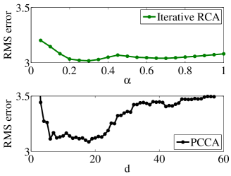
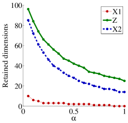
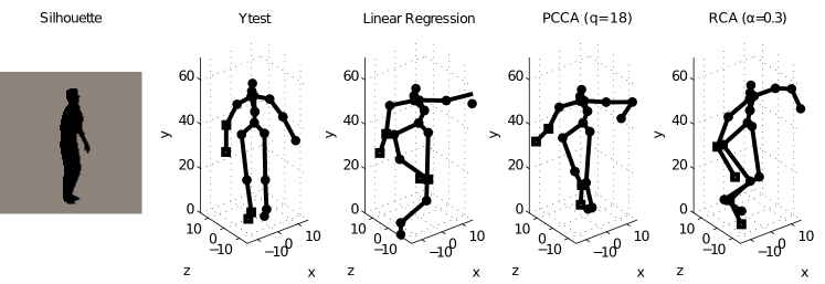
Figure 3: Comparison of iterative RCA for a shared latent space with standard CCA and a linear regression model. 3 Iterative RCA against standard probabilistic CCA with root mean square errors for reconstruction of the pose. The figure shows the error for varying $q$ (i.e. the latent dimensionality) in PCCA and varying $\alpha$ (i.e. the proportion of explained variance) in RCA. Linear regression also yields an RMS = 3.2098. 3 Latent dimensionalities on convergence, of $\mathbf{X}_{1}$, $\mathbf{X}_{2}$ and $\mathbf{Z}$ (cf. Figure 1), for varying $\alpha$. 3 Shows the silhouette and the pose predictions, alongside ground truth for frame #404, which was the frame in the test set with the largest error.

Comparison of Iterative RCA with varying $\alpha$, to PCCA with varying $q$, yields the root mean square (RMS) errors illustrated in Figure 3. Iterative RCA outperforms standard PCCA in general with the smallest difference in performance being at $q=18$ for PCCA and $\alpha=0.3$. The RMS error of RCA is robust for a wide range of large $\alpha$ values. An interesting aspect of iterative RCA is the self-regularity that the algorithm imposes on the latent dimensionalities of the shared and private components, see Figure 3. As the noise increases with $\alpha$, the eigenvalues decay faster from $\mathbf{Z}$ and $\mathbf{X}_{2}$ than from $\mathbf{X}_{1}$. Other approaches to selecting the dimensionality of the latent spaces could also be followed, but the approach of explaining a proportion of the variance with the noise seems simple and satisfactory.

5 Discussion

We have introduced residual component analysis: an algorithm for describing a low dimensional representation of the residuals of a data set given partial explanation by a covariance matrix $\Sigma$. With imaginative application our algorithm allows for novel approaches to data analysis. We illustrated this with the characterization of the difference between a treatment and control time series and an algorithm for fitting a low dimensional variant of CCA. Other forms of $\mathbf{\Sigma}$ that could be of interest include one with a sparse inverse. Sparse inverse structures capture relations between variables that are not well characterized by low rank forms. As such, the combination of sparse inverse and low rank could be a powerful one. Finally a form which reflects class structure in the data would also allow the exploration of components of the data which were not related to the class structure.

References

- Agarwal and Triggs [2006] Ankur Agarwal and Bill Triggs. Recovering 3D human pose from monocular images. IEEE Transactions on Pattern Analysis and Machine Intelligence, 28(1), 2006. doi: 10.1109/TPAMI.2006.21.
- Angelini et al. [2007] C. Angelini, D. De Canditiis, M. Mutarelli, and M. Pensky. A Bayesian approach to estimation and testing in time-course microarray experiments. Stat Appl Genet Mol Biol, 6:24, 2007.
- [3] Anonymous Author. Anonymous title.
- Bach and Jordan [2002] Francis R. Bach and Michael I. Jordan. Kernel independent component analysis. Journal of Machine Learning Research, 3:1–48, 2002.
- Bach and Jordan [2005] Francis R. Bach and Michael I. Jordan. A probabilistic interpretation of canonical correlation analysis. Technical Report 688, Department of Statistics, University of California, Berkeley, 2005.
- De Bie et al. [2005] T. De Bie, N. Cristianini, and R. Rosipal. Eigenproblems in pattern recognition. Handbook of Geometric Computing: Applications in Pattern Recognition, Computer Vision, Neuralcomputing, and Robotics, pages 129–170, 2005.
- Della Gatta et al. [2008] G. Della Gatta, M. Bansal, A. Ambesi-Impiombato, D. Antonini, C. Missero, and D. di Bernardo. Direct targets of the TRP63 transcription factor revealed by a combination of gene expression profiling and reverse engineering. Genome research, 18(6):939, 2008.
- Ek et al. [2008] Carl Henrik Ek, Jon Rihan, Philip Torr, Gregory Rogez, and Neil D. Lawrence. Ambiguity modeling in latent spaces. In Andrei Popescu-Belis and Rainer Stiefelhagen, editors, Machine Learning for Multimodal Interaction (MLMI 2008), LNCS, pages 62–73. Springer-Verlag, 28–30 June 2008.
- Kalaitzis and Lawrence [2011] Alfredo A. Kalaitzis and Neil D. Lawrence. A simple approach to ranking differentially expressed gene expression time courses through gaussian process regression. BMC Bioinformatics, 12(180), 2011. doi: 10.1186/1471-2105-12-180.
- Lawrence [2005] N. D. Lawrence. Probabilistic non-linear principal component analysis with Gaussian process latent variable models. The Journal of Machine Learning Research, 6:1816, 2005.
- Rasmussen and Williams [2006] Carl Edward Rasmussen and Christopher K. I. Williams. Gaussian Processes for Machine Learning. MIT Press, Cambridge, MA, 2006. ISBN 0-262-18253-X.
- Tipping and Bishop [1999] M. E. Tipping and C. M. Bishop. Probabilistic principal component analysis. Journal of the Royal Statistical Society. Series B (Statistical Methodology), 61(3):611–622, 1999.