Abstract

We design a dynamic rate scheduling policy of Markov type via the solution (a social optimal Nash equilibrium point) to a utility-maximization problem over a randomly evolving capacity set for a class of generalized processor-sharing queues living in a random environment, whose job arrivals to each queue follow a doubly stochastic renewal process (DSRP). Both the random environment and the random arrival rate of each DSRP are driven by a finite state continuous time Markov chain (FS-CTMC). Whereas the scheduling policy optimizes in a greedy fashion with respect to each queue and environmental state and since the closed-form solution for the performance of such a queueing system under the policy is difficult to obtain, we establish a reflecting diffusion with regime-switching (RDRS) model for its measures of performance and justify its asymptotic optimality through deriving the stochastic fluid and diffusion limits for the corresponding system under heavy traffic and identifying a cost function related to the utility function, which is minimized through minimizing the workload process in the diffusion limit. More importantly, our queueing model includes both $J$-user multi-input multi-output (MIMO) multiple access channel (MAC) and broadcast channel (BC) with cooperation and admission control as special cases. In these wireless systems, data from the $J$ users in the MAC or data to the $J$ users in the BC is transmitted over a common channel that is fading according to the FS-CTMC. The $J$-user capacity region for the MAC or the BC is a set-valued stochastic process that switches with the FS-CTMC fading. In any particular channel state, we show that each of the $J$-user capacity regions is a convex set bounded by a number of linear or smooth curved facets. The random arrival rate to each user for these systems is designed to switch with the FS-CTMC fading via admission control. At the transmit end, packets to each user are queued and served under the policy. Therefore our queueing model can perfectly match the dynamics of these wireless systems.

Key words: Processor-Sharing Queues, Random Environment, Multi-Input Multi-Output, Multiple Access Channel, Broadcast Channel, Shannon Capacity Region, Markov Fading, Doubly Stochastic Renewal Process, Utility-Maximization Scheduling, Nash Equilibrium, Concave Game, Heavy Traffic, Asymptotic Optimality, Fluid Limit, Diffusion Limit, Reflecting Diffusion with Regime-Switching

1 Introduction

In the current cellular systems, each base station is considered as a separate entity with no cooperation among base stations, infrastructure cooperation among base stations has been proposed in the literature such as [1, 33, 48], which is to consider the base stations as one end of a MIMO system that has received a great deal of attention as a method to achieve high data rates over wireless links. Thus, in this paper, we study a $J$-user MIMO MAC uplink system and a $J$-user MIMO BC downlink system. Both of them can be seen as a cellular system with multiple users and multiple cooperating base station antennas: either multiple cooperating base stations each with a single antenna or a single-cell cellular system with a multi-antenna base station or a combination thereof. In the MAC or the BC, data is buffered at the transmit end and the channel is time-varying due to multipath fading, which is a typical feature of wireless channel and brings additional complexity for system design and performance analysis. We suppose that the fading process is a FS-CTMC whose discrete time version is widely used in modeling wireless channels (see, e.g., [49, 43, 48, 22], and references therein). Therefore, the $J$-user capacity regions of the MAC and the BC are both time-varying set-valued stochastic processes driven by the FS-CTMC and in each state of the Markov chain, it is well known that one can obtain the improved capacity by cooperation, e.g., the sum of the rates at which data can be served for the $J$ users is greater than the single-user capacity for any user (see, e.g., [3]). Moreover, due to the impact of the random environmental fading factor and the cooperated design, the service rates of the corresponding queueing system for the $J$ users in the MAC or in the BC are also random processes driven by the FS-CTMC.

So, motivated by the above observations, we consider a type of generalized processor-sharing queues living in a random environment, whose job arrivals to each queue follow a DSRP. Both the random environment and the random arrival rate of each DSRP are driven by a FS-CTMC. Presently, for such a queueing system, it is not known how to choose a reasonable online rate scheduling policy to minimize the average delay for a given load and exact solutions for average delay are not available even for many simple policies, which implies that any meaningful comparison has to be done by simulations. Therefore, to make the gap between the dynamic rate scheduling and the performance optimization for the system be filled to some extent, we design a dynamic rate scheduling policy of Markov type via the solution (a social optimal Nash equilibrium point) to an optimization problem that maximizes a general utility function over each of the randomly evolving capacity regions through the Karush-Kuhn-Tucker (KKT) optimality conditions (see, e.g., [35]). Moreover, to overcome the intractability of performance evaluation for the system under the designed policy, we develop stochastic fluid and diffusion models through suitable scaling of time and space and justifying related limit theorems for a heavily loaded queueing system operating under this policy. The limit models for queue lengths (or workloads) are respectively a random process driven by the FS-CTMC and a RDRS (i.e., a reflecting stochastic differential equation (SDE) with regime-switching). In addition, we identify a cost function related to the utility function, which is minimized through minimizing the workload process in the diffusion limit and hence provides a useful means in illustrating our policy to be asymptotically optimal.

Finally, in order to incorporate the $J$-user MIMO MAC and MIMO BC into our general queueing framework, we justify that the $J$-user capacity region for the MAC or the BC in any particular channel state is a convex set formed by a number of linear or smooth curved facets through applying the method of convex optimization, the implicit function theorem, and the duality of capacity regions between the MAC and the BC. Moreover, to realize the DSRP in the MAC or in the BC, we adopt a cross-layer design methodology to switch the arrival rates with the FS-CTMC channel fading process according to the current channel state information (CSI) through admission control.

Literature Review

The randomly evolving capacity region used in designing our utility-maximization rate scheduling policy is a generalization of the so-called MIMO channel capacity region in the Shannon theoretic sense. For a single-user time-invariant channel, the Shannon capacity is defined as the maximum mutual information between input and output, which is shown by Shannon’s capacity theorem to be the maximum data rate that can be transmitted over the channel with arbitrarily small error probability. For a $J$-user time-invariant MIMO channel, the corresponding capacity region is a $J$-dimensional set of all rate vectors $(c_{1},...,c_{J})^{\prime}$ simultaneously achievable by all $J$ users. In particular, the region for the Gaussian MAC is a convex set that is the union of rate regions corresponding to every product input distribution satisfying the user-by-user power constraints (see, e.g., [14], [12], [56], [25]). The Gaussian BC differs from the Gaussian MAC in two fundamental aspects (see, e.g., [31]). In the MAC, each transmitter has an individual power constraint, whereas in the BC there is only a single power constraint on the transmitter. Moreover, signal and interference come from different transmitters in the MAC and are multiplied by different channels gains (known as the near-far effect) before being received, whereas in the BC, the entire received signal comes from the same source and therefore has the same channel gain. Nevertheless, the capacity region for the Gaussian BC can be obtained through the duality between the Gaussian MAC and the Gaussian BC (see, e.g., [31] and [25]), i.e., it is the convex hull of the union over the set of capacity regions of the dual Gaussian MACs such that the total MAC power is the same as the power in the BC. Moreover, the authors in [34] provide an analytical and numerical characterization in terms of the shape of the capacity boundaries for both the MAC and the BC.

However, in both the Gaussian MAC and the Gaussian BC, the exact characterization concerning piecewise smoothness of the capacity boundaries is not available until now, which motivates us to give more accurate analysis about the capacity region in order to apply our utility maximization rate scheduling algorithm to these wireless systems. In addition, when the $J$-user MIMO channels are stochastic and time-varying fading ones, the capacity regions have multiple definitions (see, e.g., [25]). Nevertheless, to capture the exact capacity region at each time instant for the MAC or the BC, we consider the capacity regions as a set-valued stochastic process evolving with the FS-CTMC rather than think of it as a fixed one in an average sense such as an ergodic capacity region (see, e.g., [25]).

Concerning the scheduling algorithms, the authors in [1, 3, 4] considered a quasi-static downlink channel, where the channel is assumed to be fixed for all transmissions over the period of interest. In this case, the FS-CTMC and the random packet arrival rates assumed in the current paper reduce to constants, and moreover, without considering utility and cost optimization, the authors in [1, 3, 4] designed a simple rate scheduling policy of Markov type, which was shown to be throughput-optimal for a fixed convex capacity region in [1] and a limit theorem was proved to justify the diffusion approximation of the queue length process for a heavily loaded system operating under their policy with two users in [3] and with multiple users in [4]. Their approximating model is a RBM living in the two-dimensional positive quadrant or in the general-dimensional positive orthant.

In the studies of [43, 41, 22], some scheduling policies were considered for certain heavily loaded wireless systems with finite state discrete time Markov fading process. In particular, a MaxWeight scheduling policy was considered in [43] for a generalized switch and it was shown that the workload process converges to a one-dimensional RBM and MaxWeight policy asymptotically minimizes the workload under certain conditions. Moreover, an exponential scheduling rule was designed for wireless channels in [41] and for a generalized switch in [22], which was proved to be throughput-optimal and under which, the similar results concerning the workload process were obtained and justified as in [43]. In addition, [54] designed a utility-maximizing resource allocation policy for a class of stochastic networks with concurrent occupancy of resources and established its asymptotic optimality for the associated heavily loaded queueing system. Their policy covers the generalized $c\mu$-rule in [36] and the MaxWeight policy in [43] as special cases.

The differences between the current study and those in [43, 41, 22, 54] are in three aspects as follows.

First, their scheduling policies in [43, 41, 22, 54] depend only on a fixed capacity region that is a convex polyhedral and ours depends on a time-varying and stochastic evolving capacity region process (a random environment) that, at each time instant, is a more general convex region rather than a convex polyhedral.

Second, the rates of packet arrivals to the $J$ users are random processes rather than a constant as used in [43, 41, 22, 54]. Hence our input traffic to each user is a DSRP whose particular case is the well-known doubly stochastic Poisson process (see, e.g., [8]) that is widely used to model voice, video and data source traffics in telecommunication systems and is called Markovian modulated Poisson process (MMPP) or ON/OFF source (see, e.g., [30], [37], [44], [20]) and [21])).

Third, our discussion is based on a continuous time horizon rather than a discrete one as in [43, 41, 22]. Therefore our vector-valued random service rate process depends on the FS-CTMC whose holding time at each environmental state has an important impact on the limiting processes, e.g., the limiting fluid model is a random process driven by the FS-CTMC rather than a deterministic function of time and the limiting diffusion model is a more general RDRS rather than a RBM as derived in [43, 41, 22]. If one wants to directly generalize the studies in [43, 41, 22] to the corresponding ones in a discrete time random environment, a geometric distribution may be imposed on the holding time at each environmental state.

Finally, without considering optimal dynamic scheduling with utility/cost and performance optimizations as the goals. CTMCs have been used to model the random environments in the studies of some queueing systems under certain static service disciplines, see, e.g., [13] and references therein for more details.

The rest of the paper is organized as follows. In Section 2, we introduce our generalized processor-sharing queues under random environment and design our optimal rate scheduling policy. In Section 3, we introduce our heavy traffic condition and present our main asymptotic optimality theorem. In Section 4, we illustrate the usages of our optimal policy and our main results in the $J$-user MIMO uplink and downlink wireless channels and present the associated results concerning the piecewise smoothness of capacity boundaries of the $J$-user MIMO MAC and MIMO BC. In Sections 5-6, we prove our main theorem and associated lemmas.

2 Optimizing Processor-Sharing Queues under Random Environment

2.1 Primitive Data

The queueing system under consideration is a type of generalized processor-sharing queues that live in a random environment evolving according to a stationary FS-CTMC $\alpha=\{\alpha(t),t\in[0,\infty)\}$, which takes value in a finite state space ${\cal K}\equiv\{1,...,K\}$ with generator matrix $G=(g_{il})$ ($i,l\in{\cal K}$) and

(2.3) $$g_{il}=\left\{\begin{array}[]{ll}-\gamma(i)&\mbox{if}\;\;i=l,\\ \gamma(i)q_{il}&\mbox{if}\;\;i\neq l\end{array}\right.$$

where $\gamma(i)$ is the holding rate for the chain in an environmental state $i\in\{1,...,K\}$ and $Q=(q_{il})$ is the transition matrix of its embedded discrete time Markov chain (see, e.g., [39]). Moreover, the queueing system has $J$ queues in parallel, which correspond to $J$ users for a given positive integer $J$. Each queue that is of infinite buffer capacity buffers packets (jobs) arrived for a given user. The queues can be served simultaneously by a single server with rate allocation vector $c(t)=(c_{1}(t),...,c_{J}(t))^{\prime}$ that takes values in a time-varying and randomly evolving capacity set ${\cal R}(\alpha(t))$.

Concretely, for each state $i\in{\cal K}$, ${\cal R}(i)$ is a convex set that contains the origin and has $L\;(>J)$ boundary pieces of which $J$ are $(J-1)$-dimensional linear facets along the coordinate axes while the remaining ones are in the interior of $R^{J}_{+}$ and form the so-called capacity surface denoted by ${\cal O}(i)$, which consists of $B=L-J\;(>0)$ linear or smooth curved facets $h_{k}(c,i)$ on $R_{+}^{J}$ for $k\in{\cal U}\equiv\{1,2,...,B\}$, i.e.,

(2.4) $${\cal R}(i)\equiv\left\{c\in R_{+}^{J}:\;h_{k}(c,i)\leq 0,\;k\in{\cal U}\right\}.$$

Moreover, if we let $C_{U}$ denote the sum capacity upper bound for the capacity region, then the facet in the center of the capacity surface is linear and can be expressed by

(2.5) $$h_{k_{U}}(c,i)=\sum_{j=1}^{J}c_{j}-C_{U}$$

where $k_{U}\in{\cal U}$ is the index corresponding to $C_{U}$. Moreover, we suppose that any one of the $J$ linear facets along the coordinate axes forms a $(J-1)$-user capacity region corresponding to a particular group of $J-1$ users who are the only users in the systems. Similarly, we can define the $(J-j)$-user capacity region for each $j\in\{2,...,J-1\}$. Examples of such capacity sets in two- and three-dimensional spaces for a particular state $i\in{\cal K}$ are shown in Figures 1 and 2.

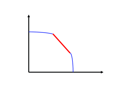
Figure 1: A 2-user capacity set in the 2-dimensional space in a particular environmental state

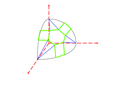
Figure 2: A 3-user capacity set in the 3-dimensional space in a particular environmental state

In addition, we suppose that the system starts empty and that there is a $J$-dimensional packet arrival process $A=\{A(t)=(A_{1}(t),...,A_{J}(t))^{\prime},t\geq 0\}$, where $A_{j}(t)$ with $j\in{\cal J}$ and $t\geq 0$ is the number of packets arrived to the $j$th queue during $(0,t]$ and the prime denotes the transpose of a vector or a matrix. For each $j\in{\cal J}$, $A_{j}(\cdot)$ is assumed to be a DSRP with random arrival rate process $\lambda_{j}(\alpha(\cdot))$ and squared coefficient of variation process $\alpha^{2}_{j}(\alpha(\cdot))\in(0,\infty)$. The packet interarrival times are assumed to be i.i.d. during the time interval corresponding to a specific environmental state $i\in{\cal K}$. Moreover, let $\{u_{j}(k),k=1,2,...\}$ denote the sequence of times between the arrivals of the $(k-1)$th and the $k$th packets to the $j$th queue and let $\{v_{j}(k),k=1,2,...\}$ denote the sequence of packet lengths (in bits) for the successive arrivals to queue $j$, which is assumed to be a sequence of strictly positive i.i.d. random variables with average packet length $1/\mu_{j}\in(0,\infty)$ and squared coefficient of variation $\beta_{j}^{2}\in(0,\infty)$. In addition, we suppose that all interarrival and service time processes are mutually (conditionally) independent when the environmental state is fixed. For each $j\in{\cal J}$ and each nonnegative constant $h$ (in bits), we use $S_{j}(\cdot)$ to denote the renewal counting process associated with $\{v_{j}(k),k=1,2,...\}$, i.e.,

(2.6) $$S_{j}(h)=\sup\left\{n\geq 0:\sum_{k=1}^{n}v_{j}(k)\leq h\right\}.$$

The reasonability about the DSRP assumption on the packet arrivals and about the i.i.d. assumption on the packet sizes in a communication system is due to the large-scale computer experiments and statistical analysis conducted by Bell Labs scientists [10], and recent findings by [20]) and [21]).

2.2 A Utility-Maximization Scheduling Algorithm and Queueing Dynamics

First of all, we remark that the service discipline used in this paper is the so-called head of line discipline under which the service goes to the packet at the head of the line for a serving queue where packets are stored in the order of their arrivals. The service rates are determined by a function of the environmental state and the number of packets in each of the queues. At each state $i\in{\cal K}$ and for a given queue length vector $q=(q_{1},...,q_{J})^{\prime}$, let $\Lambda(q,i)$ denote the corresponding rate vector (in bps) of serving the $J$ queues, which is a solution of the following utility maximization problem

(2.7) $$\max_{c\in{\cal R}(i)}\sum_{j\in{\cal J}}U_{j}(q_{j},c_{j})$$

where $c=(c_{1},...,c_{J})^{\prime}$ is a $J$-dimensional vector and $U_{j}(q_{j},c_{j})$ for each $j\in{\cal J}$ is a utility function defined on $R_{+}^{J}$, which is second-order differentiable and satisfies the following conditions

(2.8) $$U_{j}(0,c_{j})=0,$$

(2.9) $$U_{j}(q_{j},c_{j})=\Phi_{j}(q_{j})\Psi(c_{j})\;\;\mbox{is strictly increasing and concave in}\;\;c_{j}\;\;\mbox{for each}\;\;q_{j}>0,$$

(2.10) $$\frac{\partial U_{j}(q_{j},c_{j})}{\partial c_{j}}\;\;\mbox{is strictly increasing in}\;\;q_{j}\geq 0,\;\;$$

(2.11) $$\frac{\partial U_{j}(0,c_{j})}{\partial c_{j}}=0\;\;\mbox{and}\;\;\lim_{q_{j}\rightarrow\infty}\frac{\partial U_{j}(q_{j},c_{j})}{\partial c_{j}}=+\infty\;\;\mbox{for each}\;\;c_{j}>0.$$

Due to condition (2.9), we know that there must exist an optimal solution in the following form for a given $q$,

(2.14) $$\Lambda(q,i)=\left\{\begin{array}[]{ll}\Lambda^{{\cal Q}(k_{1},...,k_{m})}(q,i)^{\prime}&\mbox{if}\;\;q\in{\cal Q}(k_{1},...,k_{m})\;\;\mbox{and a given}\;\;m\in{\cal J},\\ (0,0,...,0)&\mbox{if}\;\;q=0,\end{array}\right.$$

where $k_{j}\in{\cal J}$ for each $j\in\{1,...,m\}$ and $k_{j}\neq k_{l}$ if $j\neq l$. Moreover, ${\cal Q}(k_{1},...,k_{m})$ denotes the set of all $q\in R_{+}^{J}$ that have exactly $m$ components $q_{k_{j}}$ ($j\in\{1,...,m\}$) to be zero, and the components of $\Lambda^{{\cal Q}(k_{1},...,k_{m})}(q,i)^{\prime}$ corresponding to $k_{j}$ ($j\in{\cal J}\setminus\{1,...,m\}$) consist of the optimal solution to (2.7) with the capacity region ${\cal R}(i)$ replaced by the corresponding $(J-m)$-user capacity region and all other components of $\Lambda^{{\cal Q}(k_{1},...,k_{m})}(q,i)^{\prime}$ are zero. For example, when there are only two users in the system, (2.14) is of the following form,

(2.19) $$\Lambda(q,i)=\left\{\begin{array}[]{ll}(c_{1}(q,i),c_{2}(q,i))^{\prime}&\mbox{if}\;\;q>0,\\ (c_{1}^{*}(i),0)&\mbox{if}\;\;q_{1}>0,\;\;q_{2}=0,\\ (0,c_{2}^{*}(i))&\mbox{if}\;\;q_{1}=0,\;\;q_{2}>0,\\ (0,0)&\mbox{if}\;\;q_{1}=q_{2}=0.\end{array}\right.$$

Remark 2.1

The optimal solution to (2.7) may not be unique when $q_{j}=0$ for some $j\in{\cal J}$, however, if $\Lambda_{j}(q,i)>0$ with $q_{j}=0$ for some $j\in{\cal J}$, we can reset $\Lambda_{j}(q,i)$ to zero without violating the constraints or decreasing the objective value (referred to (2.9)). Hence, whenever the solution to (2.7) is concerned, we will always suppose that $(\ref{e:zerozero})$ is true. Moreover, for each $q>0$ (and similarly, for a lower dimensional case), it follows from (2.9) that every point on the capacity surface defined in (2.4) is a Nash equilibrium point to a concave game in the sense of [40] and therefore the solution to (2.7) is a social optimal Nash equilibrium point to the concave game.

In addition, we assume that $\{U_{j}(q_{j},c_{j}),j\in{\cal J}\}$ satisfies the so-called radial homogeneity condition, i.e., for any scalar $a>0$, each $q>0$ and each $i\in{\cal K}$, its maximizer satisfies

(2.20) $$\Lambda_{j}(aq,i)=\Lambda_{j}(q,i).$$

Interested readers are referred to [54] for numerous examples of the utility function that satisfies conditions (2.8)-(2.11) and (2.20), such as, the so-called proportional fair allocation, minimal delay allocation, and $(\beta,\alpha)$-proportionally fair allocation, which are widely used in communication protocols.

2.3 The Dual Cost Minimization Problem

In this subsection, we consider the following cost minimization problem for each $i\in{\cal K}$, a given $c\in{\cal R}(i)$ and a given parameter $w\geq 0$,

(2.21) $$\min_{q}V(q,c)$$

$$\mbox{s.t.}\;\;\sum_{j=1}^{J}\frac{q_{j}}{\mu_{j}}\geq w,$$

$$\;\;\;\;\;\;\;q_{j}\geq 0\;\;\mbox{for each}\;\;j\in{\cal J}$$

where the function $V$ is defined by

(2.22) $$V(q,c)=\sum_{j=1}^{J}C_{j}(q_{j},c_{j})$$

and $C_{j}$ is the cost function associated with the utility function $U_{j}$ in (2.7), i.e.,

(2.23) $$C_{j}(q_{j},c_{j})=\frac{1}{\mu_{j}}\int_{0}^{q_{j}}\frac{\partial U_{j}(u,c_{j})}{\partial c_{j}}du.$$

In other words, when the environment is in state $i\in{\cal K}$, we try to identify a queue state $q$ corresponding to a given $c\in{\cal R}(i)$ and a given parameter $w\geq 0$ such that the total cost over the system is minimized and the (average) workload meets or exceeds $w$.

2.4 Performance Measure Processes

Let $Q_{j}(t)$ denote the queue length for the $j$th queue with $j\in{\cal J}$ at each time $t\in[0,\infty)$, i.e.,

(2.24) $$Q_{j}(t)=Q_{j}(0)+A_{j}(t)-D_{j}(t)$$

where $D_{j}(t)$ is the number of packet departures from the $j$th queue in $(0,t]$, i.e., $D_{j}(t)=S_{j}(T_{j}(t))$, where

(2.25) $$T_{j}(t)=\int_{0}^{t}\Lambda_{j}(Q(s),\alpha(s))ds$$

which denotes the cumulative amount of service (measured in bits) given to the $j$th queue up to time $t$. Moreover, let $W(t)$ denote the (expected) workload at time $t$ and $Y(t)$ denote the unused capacity up to time $t$, i.e.,

(2.26) $$W(t)=\sum_{j=1}^{J}\frac{Q_{j}(t)}{\mu_{j}},\;\;Y(t)=\sum_{j=1}^{J}\left(\int_{0}^{t}\rho_{j}(\alpha(s))ds-T_{j}(t)\right)$$

where, for each $i\in{\cal K}$, $\rho(i)=(\rho_{1}(i),...,\rho_{J}(i))^{\prime}$ is a given point on the capacity surface ${\cal O}(i)$ and it is chosen to satisfy

(2.27) $$\sum_{j=1}^{J}\rho_{j}(i)=\max_{c\in{\cal R}(i)}\left(\sum_{j=1}^{J}c_{j}\right)={\cal C}_{U}\;\;\mbox{and}\;\;\rho_{1}(i)=...=\rho_{J}(i).$$

Here we remark that the second condition in (2.27) and the separable condition in (2.10) are required in proving Lemmas 5.5-5.6. However, when only a constant environment (e.g., a pseudo channel in a wireless system) is concerned, these two conditions can be removed. Obviously,

(2.28) $$Y(t)\;\;\mbox{is non-decreasing in}\;\;t\geq 0$$

since, for each $t\geq 0$, we have

(2.29) $$\sum_{j=1}^{J}\Lambda_{j}(Q(t),\alpha(t))\leq\sum_{j=1}^{J}\rho_{j}(\alpha(t)).$$

3 Main Theorem: Asymptotic Optimality

In this section, we present the optimality result for our scheduling policy by considering the operation of the queueing system in the asymptotic regime where it is heavily loaded. Concretely, we define three sequences of diffusion-scaled processes $\hat{Q}^{r}(\cdot)$, $\hat{W}^{r}(\cdot)$ and $\hat{Y}^{r}(\cdot)$ by

(3.30) $$\hat{Q}_{j}^{r}(t)\equiv\frac{Q_{j}^{r}(r^{2}t)}{r},\;\;\;\hat{W}^{r}(t)\equiv\frac{W^{r}(r^{2}t)}{r},\;\;\;\hat{Y}^{r}(t)\equiv\frac{Y^{r}(r^{2}t)}{r}$$

for each $t\geq 0$ and $j\in{\cal J}$, which associate with a sequence of independent Markov processes $\{\alpha^{r}(\cdot),r\in\{1,2,...\}\}$. These systems indexed by $r$ all have the same basic structure as described in the last section except the arrival rates $\lambda^{r}_{j}(i)$ and the holding time rates $\gamma^{r}(i)$ for all $i\in{\cal K}$, which may vary with $r\in\{1,2,...\}$ and satisfy the following heavy traffic condition

(3.31) $$r\left(\lambda_{j}^{r}(i)-\lambda_{j}(i)\right)\rightarrow\theta_{j}(i)\;\;\mbox{as}\;\;r\rightarrow\infty,\;\;\gamma^{r}(i)=\frac{\gamma(i)}{r^{2}}$$

for each $j\in{\cal J}$, where $\theta_{j}(i)\in R$ are some constants and $\lambda_{j}(i)\equiv\mu_{j}\rho_{j}(i)$ are the nominal average packet arrival rates when the channel is in state $i\in{\cal K}$.

Note that, due to the heavy traffic condition in (3.31) for the $r$th environmental state process $\alpha^{r}(\cdot)$ with $r\in\{1,2,...\}$, we know that $\alpha^{r}(r^{2}\cdot)$ and $\alpha(\cdot)$ equal each other in distribution since they own the same generator matrix (see, e.g., the definition in pages 384-388 of [39]). Hence, in the sense of distribution, all of the systems indexed by $r\in\{1,2,...\}$ in (3.30) share the same random environment over any time interval $[0,t]$.

Moreover, let $B^{E}(\cdot)$ and $B^{S}(\cdot)$ denote the two independent $J$-dimensional standard Brownian motions, and for each $i\in{\cal K}$, let

(3.32) $$\lambda(i) = (\lambda_{1}(i),...,\lambda_{J}(i))^{\prime},$$

(3.33) $$\rho(i) = \left(\rho_{1}(i),...,\rho_{J}(i)\right)^{\prime},$$

(3.34) $$\theta(i) = (\theta_{1}(i),...,\theta_{J}(i))^{\prime},$$

(3.35) $$\Gamma^{E}(i) = \left(\Gamma^{E}_{kl}(i)\right)_{J\times J}\equiv\mbox{diag}\left(\lambda_{1}(i)\alpha_{1}^{2}(i),...,\lambda_{J}(i)\alpha^{2}_{J}(i)\right),$$

(3.36) $$\Gamma^{S}(i) = \left(\Gamma^{S}_{kl}(i)\right)_{J\times J}\equiv\mbox{diag}\left(\lambda_{1}(i)\beta_{1}^{2},...,\lambda_{J}(i)\beta_{J}^{2}\right),$$

(3.37) $$H^{e}(t) = \left(H^{e}_{1}(t)^{\prime},...,H^{e}_{J}(t)\right)^{\prime}\;\;\mbox{with}\;\;e\;\;\mbox{denotes}\;\;E\;\;\mbox{or}\;\;S,$$

(3.38) $$H^{e}_{j}(t) = \int_{0}^{t}\left(\Gamma^{e}_{jj}(\alpha(s))\right)^{\frac{1}{2}}dB^{e}_{j}(s).$$

In addition, let $\hat{Q}^{r,G}(\cdot)$ and $\hat{W}^{r,G}(\cdot)$ denote the diffusion-scaled queue-length and workload processes under an arbitrarily feasible rate scheduling policy $G$, e.g., a simple Markovian policy as studied in [4] or a policy $\Lambda^{G}(Q^{r}(t),\alpha(t))$ that may not be the optimal solution to the utility maximization problem (2.7). Then we have the following theorem.

Theorem 3.1

Suppose $Q^{r}(0)=0$ for all $r\in\{1,2,...\}$ and the heavy traffic condition (3.31) holds, then under the scheduling policy (2.14), we have the claims as stated in the following two parts:
Part A: Along $r\in\{1,2,...\}$, the following convergence in distribution is true,

(3.39) $$(\hat{Q}^{r}(\cdot),\hat{W}^{r}(\cdot),\hat{Y}^{r}(\cdot))\Rightarrow(\hat{Q}(\cdot),\hat{W}(\cdot),\hat{Y}(\cdot))$$

and the limits $\hat{Q}(\cdot),\hat{W}(\cdot)$ and $\hat{Y}(\cdot)$ are continuous a.s., which satisfy the following RDRS

(3.40) $$\hat{W}(t)=\hat{X}(t)+\hat{Y}(s)\geq 0$$

where

(3.41) $$d\hat{X}(t)=\sum_{j=1}^{J}\frac{1}{\mu_{j}}\left(\theta_{j}(\alpha(t))dt+dH_{j}^{E}(t)+dH^{S}_{j}(t)\right)$$

Moreover, $(\hat{W}(\cdot),\hat{Y}(\cdot))$ is the unique solution of (3.40) with the following complementary property:

1. $\hat{Y}(0)=0$,

2. $\hat{Y}(\cdot)$ is non-decreasing,

3. $\hat{Y}(\cdot)$ can increase only at a time $t\in[0,\infty)$ that $\hat{W}(t)=0$.

In addition, we have

(3.42) $$\hat{Q}(t)=q^{*}(\hat{W}(t),\rho(\alpha(t)))$$

with $q^{*}(w,\rho(i))$ being the solution to the cost minimization problem (2.21) in terms of each given $w$ and $i\in{\cal K}$.
Part B: The workload $\hat{W}(\cdot)$ and the cost $\sum_{j=1}^{J}C_{j}(\hat{Q}_{j}(\cdot),\rho(\alpha(\cdot)))$ are minimal with probability one in the sense that, for all $t\geq 0$,

(3.43) $$\liminf_{r\rightarrow\infty}\hat{W}^{r,G}(t)\geq\hat{W}(t),$$

(3.44) $$\liminf_{r\rightarrow\infty}\sum_{j=1}^{J}C_{j}(\hat{Q}_{j}^{r,G}(t),\rho_{j}(\alpha(t)))\geq\sum_{j=1}^{J}C_{j}(\hat{Q}_{j}(t),\rho_{j}(\alpha(t))).$$

Remark 3.1

Comparing with the RBM widely studied in queueing literature, the RDRS model derived in (3.40) exhibits its new feature in the sense that it corresponds to a more realistic FS-CTMC fading process in certain applications such as in a wireless system and indicates that the random process $\alpha(\cdot)$ is a non-ignorable random environmental factor to the system performance even in the limiting approximation model. From the model, we can also see that, when a constant environment (e.g., a quasi-static channel in a wireless system) is concerned, the model in (3.40) reduces to a RBM since the state process $\alpha(\cdot)$ keeps a constant. Moreover, by the discussions in [11], [18], [17], and [26], we know that the unique solution $(\hat{W}(t),\hat{Y}(t))$ to (3.40) can be represented by $(\hat{W},\hat{Y})=(\Phi(\hat{X}),\Psi(\hat{X}))$, where $\Phi(\cdot)$ and $\Psi(\cdot)$ are Lipschitz continuous mappings. In addition, a RDRS is different from a conventional SDE since its drift and diffusion coefficients are not adapted to the filtration generated by the driving Brownian motions. This type of SDEs without boundary reflections has received a great attention in the area of financial engineering (see, e.g., [57]).

4 Applications to $J$-user MIMO Uplink and Downlink Wireless Channels

In this section, we apply the discussions in the previous sections to a cellular system where base stations cooperate among noise-free infinite capacity links. We do not make any distinction between a single-cell cellular system having multiple base-station antennas and the traditional cellular system with cooperating single-antenna base stations. Here, the cooperation means that the base stations can perform joint beamforming and/or power control but there is a constraint on the total power that the base stations can share. Therefore, our wireless system can be considered consisting of a base station having $M$ antennas and $J$ users (mobiles), each of which has $N$ antennas. Thus the uplink channel can be modeled as a $J$-user MIMO MAC and the downlink channel can be modeled as a $J$-user MIMO BC (see, e.g., Figure 3).

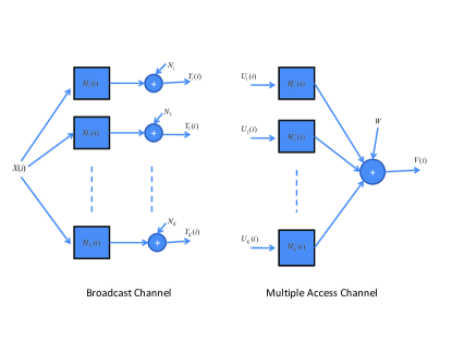
Figure 3: The BC and MAC channels in a particular environmental state

The channel fading is supposed to obey the stationary FS-CTMC $\alpha=\{\alpha(t),t\in[0,\infty)\}$ that is described in the previous sections. Moreover, we suppose that the receive or transmit end (the cooperating base stations) has perfect CSI. For each channel state $i\in{\cal K}$, we let $H_{j}(i)$ ($j\in{\cal J}\equiv\{1,...,J\}$) denote the downlink channel matrix from the base station to user $j$. Assuming the same channel is used on the uplink and downlink, then the uplink matrix of user $j$ is $H^{\dagger}_{j}(i)$ that is the conjugate transpose of $H_{j}(i)$.

Moreover, at the transmit end, arriving packets for each user are buffered before transmission and the rate of arrivals is a random process that switches with the FS-CTMC channel fading through admission control. Therefore, the processor-sharing queues presented in the previous section can be used to model the channel dynamics for both $J$-user MIMO MAC and $J$-user MIMO BC. The remaining issue is about how to characterize the MAC and BC capacity region processes, which is also a central topics in information theory literature.

4.1 The MIMO MAC Capacity Region

In the MAC and for each channel state $i\in{\cal K}$, let $U_{j}(i)\in{\cal C}^{N\times 1}$ be the transmitted signal of user $j$, where ${\cal C}^{N\times 1}$ denotes the $N\times 1$ complex matrix, and let $V(i)\in{\cal C}^{M\times 1}$ denote the received signal, $W\in{\cal C}^{M\times 1}$ denote the noise vector where $W\sim\bar{N}(0,I)$ is circularly symmetric complex Gaussian with identity covariance (note that the notation $W$ here has the different meaning from the workload process $W(t)$ defined in (2.26)). Then the received signal at the base station is equal to

(4.45) $$V(i)=H^{\dagger}(i)U^{\prime}(i)+W$$

where $H^{\dagger}(i)=[H_{1}^{\dagger}(i),...,H_{J}^{\dagger}(i)]$ and $U(i)=[U^{\prime}_{1}(i),...U^{\prime}_{J}(i)]$ (see, e.g., Figure 3). Moreover, each user $j$ is subject to an individual power constraint $P_{j}$. The transmit covariance matrix of user $j$ is defined to be $\Gamma_{j}(i)\equiv E[U_{j}(i)U_{j}^{\dagger}(i)]$. The power constraint implies that Tr$(\Gamma_{j}(i))\leq P_{j}$ for $j\in{\cal J}$. During the period of each channel state $i\in{\cal K}$, it follows from [25] and [56] that the MAC capacity region is a $J$-dimensional closed convex set in $R_{+}^{J}\equiv\{c\in R^{J}:c_{j}\geq 0,j\in{\cal J}\}$, i.e.,

(4.46) $${\cal R}(i)={\cal C}_{MAC}(P_{1},...,P_{J},H^{\dagger}(i))=$$

$$\bigcup_{\{\Gamma_{j}(i)\geq 0,\mbox{Tr}(\Gamma_{j}(i))\leq P_{j},j\in{\cal J}\}}\left\{c\in R^{J}_{+}:\sum_{j\in S}c_{j}\leq\frac{1}{2}\mbox{log}\left|I+\sum_{j\in S}H_{j}^{\dagger}(i)\Gamma_{j}(i)H_{j}(i)\right|,\forall\;\;S\subset{\cal J}\right\}$$

where $S$ is a subset of ${\cal J}$ and $|\cdot|$ denotes the determinant of a matrix. Moreover, every point in ${\cal R}(i)$ can be achieved by Shannon’s source coding theorem and successive decoding (see, e.g., [24] and [25]). However, in designing a utility maximization based rate scheduling policy, we need to know more detailed boundary characterization of the MAC capacity region since it frequently relies on the KKT optimality conditions (see, e.g., [35] and [34]). Thus we have the following lemma.

Lemma 4.1

For the $J$-user MIMO MAC and each channel state $i\in{\cal K}$, ${\cal R}(i)$ contains the origin and has $L$ linear or smooth curved facets with $L$ given by

(4.47) $$L=J!+\sum_{j=2}^{J}C_{J}^{j}(J-j+1)!+J.$$

Moreover, $J$ of these pieces are $(J-1)$-dimensional linear facets along the coordinate axes while the remaining $B=L-J$ ones are in the interior of $R^{J}_{+}$ and form ${\cal O}(i)$, which are linear or smooth curved facets $h_{k}(c,i)$ on $R_{+}^{J}$ for $k\in{\cal U}\equiv\{1,2,...,B\}$, i.e.,

(4.48) $${\cal R}(i)\equiv\left\{c\in R_{+}^{J}:\;h_{k}(c,i)\leq 0,\;k\in{\cal U}\right\}.$$

Moreover, if $C_{MAC}(P,H(i))$ is used to denote the sum capacity upper bound for the MAC capacity region, then

(4.49) $$h_{k_{MAC}}(c,i)=\sum_{j=1}^{J}c_{j}-C_{MAC}(P,H(i))$$

where $k_{MAC}\in{\cal U}$ is the index corresponding to $C_{MAC}(P,H(i))$.

Example 4.1

For the MAC channel and each $i\in{\cal K}$, when $J=2$ and $N=1$ (i.e., each of the user’s mobiles has only single transmit antenna), it follows from [25] that

$$g_{1}(c,i)=c_{1}-\log\left|I+H_{1}^{\dagger}(i)P_{1}H_{1}(i)\right|,$$

$$g_{2}(c,i)=c_{1}+c_{2}-\log\left|I+H_{1}^{\dagger}(i)P_{1}H_{1}(i)+H_{2}^{\dagger}(i)P_{2}H_{2}(i)\right|,$$

$$g_{3}(c,i)=c_{2}-\log\left|I+(I+H_{1}^{\dagger}(i)P_{1}H_{1}(i))^{-1}H_{2}^{\dagger}(i)P_{2}H_{2}(i)\right|.$$

4.2 The MIMO BC Capacity Region

In the MIMO BC and for each channel state $i\in{\cal K}$, let $X(i)\in{\cal C}^{M\times 1}$ denote the transmitted vector signal from the base station and let $Y_{j}(i)\in{\cal C}^{N\times 1}$ be the received signal at the user $j$. The noise at user $j$ is represented by $N_{j}\in{\cal C}^{N\times 1}$ and is assumed to be circularly symmetric complex Gaussian noise $(N_{j}\sim N(0,I))$. The received signal of user $j$ (see, e.g., Figure 3) is equal to

$$Y_{j}(i)=H_{j}(i)X(i)+N_{j}.$$

The transmit covariance matrix of the input signal is $\Gamma_{X}(i)\equiv E\left[X(i)X^{\dagger}(i)\right]$. The base station is subject to an average power constraint, which implies that Tr($\Gamma_{X}(i))\leq P$. During each channel state $i\in{\cal K}$, the $J$-user MIMO BC capacity region denoted by ${\cal R}(i)$ can be calculated by the duality of the MAC and the BC in [31] and [25], where the BC capacity region is obtained by taking the convex hull of the union over the set of capacity regions of the dual MIMO MACs such that the total MAC power is the same as the power in the BC, i.e.,

(4.50) $${\cal R}(i)={\cal C}_{BC}(P,H(i))=\bigcup_{\{(P_{1},...,P_{J}):\sum_{j=1}^{J}P_{j}=P\}}{\cal C}_{MAC}(P_{1},...,P_{J},H^{\dagger}(i)).$$

Moreover, the Dirty Paper Coding (DPC) proposed in [15] achieves the capacity for the MIMO BC (see, e.g., [50]). In particular, if each user has only single receive antenna, we have the following lemma.

Lemma 4.2

For the $J$-user MIMO BC with $N=1$, each $i\in{\cal K}$ and $L$ given in (4.47), ${\cal R}(i)$ contains the origin and has $L$ boundary pieces of which $J$ are ($(J-1)$-dimensional linear facets along the coordinate axes while the remaining $B=L-J$ ones are in the interior of $R^{J}_{+}$ and form ${\cal O}(i)$, which are linear or smooth curved facets $h_{k}(c,i)$ on $R_{+}^{J}$ for $k\in{\cal U}\equiv\{1,2,...,B\}$, i.e.,

(4.51) $${\cal R}(i)\equiv\left\{c\in R_{+}^{J}:\;h_{k}(c,i)\leq 0,\;k\in{\cal U}\right\}.$$

Moreover, if $C_{Sato}(P,H(i))$ denotes the sum capacity upper bound (called the Sato upper bound) for the BC capacity region, then

(4.52) $$h_{k_{Sato}}(c,i)=\sum_{j=1}^{J}c_{j}-C_{Sato}(P,H(i))$$

where $k_{Sato}\in{\cal U}$ is the index corresponding to $C_{Sato}(P,H(i))$.

Remark 4.1

The concept of Sato upper bound of the $J$-user MIMO BC can be found in such as [25], [9], [47], [45], [55]. Moreover, here we conjecture that, in the MIMO BC channel, if each user has multiple receive antennas, the corresponding property stated in the lemma should also be true.

Example 4.2

Considering the BC channel with $J=2$ and $N=1$ for each $i\in{\cal K}$, we can derive $h_{k}(c,i)$ explicitly for $k=1,2,3$ by employing the results in [25], [46], [50] as follows

$$h_{1}(c,i) = e^{2(c_{1}+c_{2})}-\left|I+\left(H_{1}^{\dagger}(i)H_{1}(i)-H_{2}^{\dagger}(i)H_{2}(i)\right)\right.$$

$$\frac{e^{2c_{1}}-1}{|H_{111}|^{2}(i)+|H_{122}|^{2}(i)}+\left.H_{2}^{\dagger}(i)H_{2}(i)P\right|^{2},$$

(4.54) $$h_{2}(c,i) = c_{1}+c_{2}-{\cal C}_{\mbox{Sato}}(P,H(i)),$$

$$h_{3}(c,i) = e^{2(c_{1}+c_{2})}-\left|I+\left(H_{2}^{\dagger}(i)H_{2}(i)-H_{1}^{\dagger}(i)H_{1}(i)\right)\right.$$

$$\frac{e^{2c_{2}}-1}{|H_{211}|^{2}(i)+|H_{222}|^{2}(i)}+\left.H_{1}^{\dagger}(i)H_{1}(i)P\right|^{2}.$$

5 Proof of Theorem 3.1

To be convenient for readers, we first outline the proof of Theorem 3.1, which consists of the following five parts.

Firstly, in Subsection 5.1, we first justify a dual relationship between the utility-maximization problem in (2.7) and the cost-minimization problem in (2.21), which is summarized in Lemma 5.2. Then we prove a claim in Lemma 5.3, which states that when the system state is close to the unique optimal solution to the cost minimization problem (called a fixed point), the capacity of the system will be fully utilized. The claims stated in Lemmas 5.2-5.3 are similar to their counterparts in [54], nevertheless, their concrete proofs are different due to the different problem formulations and the difference of the capacity constraints between the two studies.

Secondly, in Subsection 5.2, we present an equivalent queueing model due to the assumption (3.31) imposed on the FS-CTMC and justify a functional central limit theorem (Lemma 5.4) for a DSRP whose arrival rate process is driven by the FS-CTMC. The main idea used in proving Lemma 5.4 is stemmed from the related discussion in [18], [17] and the concrete proving techniques include the conventional functional central limit theorem (see, e.g., [28] and [38]), random change of time lemma (see, e.g., [5]), establishment of oscillation inequality (see, e.g., [18], [17]), equivalent conditions of relative compactness and Skorohod representation theorem (see, e.g., [23]), and etc.

Thirdly, in Subsection 5.3, we derive the fluid limit processes for the physical processes under fluid scaling in Lemma 5.5 and study the asymptotic behavior for the fluid limit processes as time evolves in Lemma 5.6. Fluid limits are widely used as an intermediate step in justifying diffusion approximations (see, e.g., [7], [43], [54], [19], [3], [4], and references therein). Nevertheless, our fluid limit is a random process driven by the FS-CTMC rather than a deterministic function of time as obtained in the existing studies. This new feature brings us additional complexity in proving Lemma 5.5 and Lemma 5.6, e.g., comparing with the study in [54], it requires more technical treatment in handling the FS-CTMC based jumps for the constructed Lyapunov function. Therefore, by noticing this new feature and the difference between our optimal scheduling policy and the one in [54], we develop a theory through combining and generalizing the discussions in [54], [16], [3], and [4] to finish the justifications of Lemma 5.5 and Lemma 5.6.

Fourthly, in Subsection 5.4, we study the convergence of the workload and queue length processes on a finer time-scale, which is an important step in justifying the main result of the paper. This method has appeared in queueing literature for a while (see, e.g., [6], [54], [43], [36], [41], and etc.) The main difference between ours and the existing works is as follows: all the processes concerned in our study involve the jumps introduced by the random environment and in the meanwhile the processes in existing studies do not involve this type of jumps. Therefore we develop a scheme and incorporate it into the framework as used in [54] to finish the proof of the convergence properties for the processes on a finer time-scale.

Finally, in Subsection 5.5, we combine the results obtained in the previous subsections with the uniqueness of solution to an associated Skorohod problem and the minimality of the Skorohod problem to provide a proof for Theorem 3.1. This type of techniques have been used in the studies concerning network scheduling (see, e.g., [54], [43], [36], [41], and etc.) Nevertheless, our justification logic and technical treatment are somewhat different.

5.1 Preliminary Lemmas on the Utility-Maximization and Dual Cost Minimization Problems

Lemma 5.1

Consider the utility-maximization problem in (2.7) and suppose conditions (2.8)-(2.11) and (2.20) are imposed, then for a sequence of queue states, $\{q^{l},l=1,2,...\}$, which satisfies $q^{l}\rightarrow q\in R_{+}^{J}$ as $l\rightarrow\infty$, we have

(5.56) $$\Lambda_{j}(q^{l},i)\rightarrow\Lambda_{j}(q,i)\;\;\mbox{as}\;\;l\rightarrow\infty$$

for each $i\in{\cal K}$ and any $j\in{\cal J}$ such that $q_{j}>0$.

Proof. Consider each specific state $i\in{\cal K}$, then the proof can be accomplished similarly as for Lemma 6.2 in [53] and hence we omit it. $\Box$

Lemma 5.2

For each state $i\in{\cal K}$, the following claims are true.

1. Under the policy in (2.14) and the associated convention, if $c^{*}=\rho(i)$ is an optimal solution to the maximization problem in (2.7) with a queue state $q$ in the utility function. Then $q^{*}=q$ must be the optimal solution to the minimization problem in (2.21) with $c=c^{*}$ in the cost function and with $w=\sum_{j=1}^{J}q^{*}_{j}/\mu_{j}$ in the constraints.

2. Conversely, if $q^{*}$ is the optimal solution to the minimization problem in (2.21) with $w>0$ and $\Lambda(q^{*},i)=\rho(i)$ for each $i\in{\cal K}$ in the cost function. Then $q^{*}>0$ and $\Lambda^{*}(q^{*},i)=\Lambda(q^{*},i)$ must be an optimal solution to the maximization problem in (2.7) with $q=q^{*}$ in the utility function.

Proof. First of all, without loss of generality, we suppose that $q>0$. Then it follows from the KKT optimality conditions (see, e.g., [35]) that the solution to the utility maximization problem in (2.7) can be obtained through the following equations,

(5.57) $$c_{j}\left(\frac{\partial U_{j}(q_{j},c_{j})}{\partial c_{j}}+\sum_{k=1}^{B}\eta_{k}\frac{\partial h_{k}(c,i)}{\partial c_{j}}\right)=0\;\;\mbox{for}\;\;j\in{\cal J},$$

(5.58) $$\eta_{k}h_{k}(c,i)=0\;\;\mbox{for each}\;\;k\in{\cal U}$$

where $B$ and ${\cal U}$ are defined in (2.4), $\eta_{k}\geq 0$ for all $k\in{\cal U}$ are the Lagrangian multipliers and $h_{k}(c,i)$ for each $k\in{\cal U}$ and $i\in{\cal K}$ is defined in (2.4). Similarly, the solution to the cost minimization problem (2.21) can be obtained through the following equations,

(5.59) $$q_{j}\left(\frac{\partial C_{j}(q_{j},c_{j})}{\partial q_{j}}+\frac{\theta}{\mu_{j}}\right)=0\;\;\mbox{for each}\;\;j\in{\cal J},$$

(5.60) $$\theta\left(w-\sum_{j=1}^{J}\frac{q_{j}}{\mu_{j}}\right)=0,$$

where $\theta\geq 0$ is the Lagrangian multiplier. Moreover, it follows from (2.23) that

(5.61) $$\frac{\partial C_{j}(q_{j},c_{j})}{\partial q_{j}}=\frac{1}{\mu_{j}}\frac{\partial U_{j}(q_{j},c_{j})}{\partial c_{j}}.$$

Thus, based on the above facts, the claim in the first part of the lemma can be proved as follows. By condition (2.9), we know that $\sum_{j=1}^{J}U_{j}(q_{j},c_{j})$ is strictly concave in $c$ for each $q>0$. Therefore $c^{*}=\rho(i)$ is the unique optimal solution to the utility maximization problem in (2.7) for the given $q>0$ in the utility function, which satisfies (5.57)-(5.58). Thus, if we take

$$\theta=-\sum_{k=1}^{B}\eta_{k}\frac{\partial h_{k}(\rho(i),i)}{\partial c_{j}},$$

then it follows from (5.57) and (5.61) that (5.59) holds. Due to condition (2.11), we know that $V(q,c)$ is strictly convex in $q$ for each $c>0$. So the cost minimization problem in (2.21) has a unique optimal solution $q^{*}=q$ when $c=c^{*}=\rho(i)$ is in the cost function and $w=\sum_{j=1}^{J}q^{*}_{j}/\mu_{j}$ is in the constraints.

Conversely, the claim in the second part of the lemma can be proved as follows. Due to the conditions (2.10)-(2.11) and the relationship (2.23), we know that $V(q,\rho(i))$ is strictly convex in $q$. Therefore $q^{*}$ is the unique optimal solution to the cost minimization problem (2.21) with $\Lambda(q^{*},i)=\rho(i)$. Thus we can prove $q^{*}>0$ by showing a contradiction.

In fact, without loss of generality, we suppose that there is some $m\in{\cal J}$ with $m<J$ such that $q^{*}\in{\cal Q}(k_{1},...,k_{m})$ with $k_{1}\neq 1$ and $k_{m}=J$, where ${\cal Q}(k_{1},...,k_{m})$ is defined in (2.14). Then we can construct a $2$-dimensional line for some constant $\epsilon\geq w$,

(5.62) $$P_{1}:\;\;\frac{q_{1}}{\mu_{1}}+\frac{q_{J}}{\mu_{J}}+\sum_{j\neq 1,J,j\in{\cal J}}\frac{q^{*}_{j}}{\mu_{j}}=\epsilon\geq w$$

such that it passes through the point $q^{*}$. Now it follows from (2.23) that the function $f(q_{1},\rho(i))$ ($=V(q,\rho(i))$) with the constraint $P_{1}$ for all $q=(q_{1},q_{2}^{*},...,q_{J-1}^{*},q_{J})^{\prime}\in{\cal R}_{+}^{J}$) is of the following derivative function in $q_{1}\in{\cal R}_{1}^{+}$,

(5.63) $$\;\;\;\;\frac{\partial f(q_{1},\rho(i))}{\partial q_{1}} = \frac{1}{\mu_{1}}\frac{\partial U_{1}(q_{1},\rho_{1}(i))}{\partial c_{1}}-\frac{1}{\mu_{1}}\frac{\partial U_{J}((\epsilon-\frac{q_{1}}{\mu_{1}}-\sum_{j\neq 1,J,j\in{\cal J}}\frac{q^{*}_{j}}{\mu_{j}})\mu_{J},\rho_{J}(i))}{\partial c_{J}},$$

which is strictly increasing in $q_{1}\in{\cal R}_{1}^{+}$ due to (2.10). Moreover, it follows from (5.63) and (2.11) that

(5.64) $$\frac{\partial f(0,\rho(i))}{\partial q_{1}}=-\frac{1}{\mu_{1}}\frac{\partial U_{J}((\epsilon-\sum_{j\neq 1,J,j\in{\cal J}}\frac{q^{*}_{j}}{\mu_{j}})\mu_{J},\rho_{J}(i))}{\partial c_{J}}<0,$$

(5.65) $$\frac{\partial f(q_{1}^{*},\rho(i))}{\partial q_{1}}=\frac{1}{\mu_{1}}\frac{\partial U_{1}(q^{*}_{1},\rho_{1}(i))}{\partial c_{1}}>0.$$

Then, by (5.64) and (5.65), we know that there is a $\tilde{q}_{1}\in(0,q_{1}^{*})$ such that

(5.66) $$\frac{\partial f(\tilde{q}_{1},\rho(i))}{\partial q_{1}}=0$$

which implies that, on the curve $f(q,\rho(i))$ with $q=(q_{1},q_{2}^{*},...,q_{J-1}^{*},q_{J})^{\prime}\in R^{J}_{+}$, there exists a minimal point $\tilde{q}\in{\cal R}_{+}^{J}$ with $\tilde{q}=(\tilde{q}_{1},q_{2}^{*},...,q_{J-1}^{*},\tilde{q}_{J})^{\prime}$ such that $V(\tilde{q},\rho(i))<V(q^{*},\rho(i))$

$$\tilde{q}_{J}=\left(\epsilon-\frac{\tilde{q}_{1}}{\mu_{1}}-\sum_{j\neq 1,J,j\in{\cal J}}\frac{q^{*}_{j}}{\mu_{j}}\right)\mu_{J}.$$

This contradicts the assumption that $q^{*}$ is the optimal solution to the cost minimization problem in (2.21). Hence we can conclude that $q^{*}>0$.

Finally, if $q^{*}$ is the optimal solution to (2.21) with $c=\Lambda(q^{*},i)=\rho(i)$ in the cost function, we see that (5.59)-(5.60) hold with $q=q^{*}$ and $c=\Lambda(q^{*},i)=\rho(i)$. Therefore we can take $\eta_{k_{U}}=\theta$ and $\eta_{k}=0$ when $k\neq k_{U}$ in (5.57)-(5.58) since $q^{*}>0$ and $\rho$ is on the curve $h_{k_{U}}(c,i)=0$. Hence $\Lambda^{*}(q^{*},i)=\Lambda(q^{*},i)=\rho(i)$ for each $i\in{\cal K}$ is an optimal solution to (2.7) with $q=q^{*}$ in the utility function. $\Box$

Next, let $\|\cdot\|$ denote the norm of a vector $q\in R^{J}$ in the sense that $\|q\|=\sum_{j=1}^{J}|q_{j}|$. Then we have the following lemma.

Lemma 5.3

For each state $i\in{\cal K}$, the following claims are true.

1. The cost minimization problem (2.21) has a unique optimal solution $q^{*}=q$ when $c=\rho(i)$ is in the cost function, and moreover, $q^{*}(w,\rho(i))$ is continuous in terms of $w$.

2. Assuming that, for any given constant $\epsilon>0$, there exists another constant $\sigma>0$, which depends only on $\epsilon$, such that, for any $q\in{\cal V}(\epsilon,\sigma,i)$ with

   (5.67) $${\cal V}(\epsilon,\sigma,i)\equiv\left\{q\in R_{+}^{J}:\left\|q-q^{*}(w,\rho(i))\right\|\leq\sigma\;\;\mbox{and}\;\;w=\sum_{j=1}^{J}\frac{1}{\mu_{j}}q_{j}\;\;\geq\epsilon\right\},$$

   we have

   (5.68) $$\sum_{j=1}^{J}\Lambda_{j}(q,i)=\sum_{j=1}^{J}\rho_{j}(i).$$

Remark 5.1

The unique optimal solution $q^{*}(w,\rho(i))$ will be referred to as a fixed point in the following discussion.

Proof. For the first part in the lemma, we have the following observations. Due to condition (2.11), we know that $V(q,c)$ is strictly convex in $q$ for each $c>0$. So the cost minimization problem in (2.21) has a unique optimal solution $q^{*}=q$ when $c=\rho(i)$ is in the cost function. Moreover, the continuity of $q^{*}(w,\rho(i))$ in terms of $w$ for each $i\in{\cal K}$ can be proved similarly as in [54].

For the second part in the lemma, it can be proved by showing a contradiction. As a matter of fact, if the claim is not true for some $i\in{\cal K}$ and some $\epsilon>0$, then for a sequence of $\sigma^{l}\downarrow 0$ along $l\in\{1,2,...\}$, there is a sequence of states $\tilde{q}^{l}\in{\cal V}(\epsilon,\sigma^{l},i)$ with $l=1,2,...$ satisfying

(5.69) $$\left\|\tilde{q}^{l}-q^{*}(\tilde{w}^{l},\rho(i))\right\|\rightarrow 0\;\;\mbox{as}\;\;l\rightarrow\infty,$$

(5.70) $$\tilde{w}^{l}=\sum_{j=1}^{J}\frac{1}{\mu_{j}}\tilde{q}_{j}^{l}\geq\epsilon\;\;\mbox{for all}\;\;l=1,2,...$$

such that

(5.71) $$\sum_{j=1}^{J}\Lambda_{j}(\tilde{q}^{l},i)<\sum_{j=1}^{J}\rho_{j}(i)\;\;\mbox{for all}\;\;l=1,2,...$$

Otherwise, if there is some $l_{0}\in\{1,2,...\}$ such that ${\cal V}(\epsilon,\sigma^{l},i)$ are empty for all $l\geq l_{0}$, then (5.68) is automatically true for the given $i\in{\cal K}$ and $\epsilon>0$, which is a contradiction. Now, let

(5.72) $$q^{l}=(\epsilon/\tilde{w}^{l})\tilde{q}^{l}\;\;\mbox{so that}\;\;w^{l}=\sum_{j=1}^{J}\frac{q_{j}^{l}}{\mu_{j}}=\epsilon\;\;\mbox{for all}\;\;l=1,2,...,$$

then it follows from (5.69)-(5.70), (5.72), (2.20) and Lemma 5.2 that, along $l\in\{1,2,...\}$,

(5.73) $$q^{l}=\frac{\epsilon q^{*}(\tilde{w}^{l},\rho(i))}{\tilde{w}^{l}}+\frac{\epsilon}{\tilde{w}^{l}}\left(\tilde{q}^{l}-q^{*}(\tilde{w}^{l},\rho(i))\right)\rightarrow\hat{q}=q^{*}(\epsilon,\rho(i))>0,$$

which implies that $q^{l}>0$ for all large enough $l\in\{1,2,...\}$, and moreover, we also have

(5.74) $$\frac{\epsilon q^{*}(\tilde{w}^{l},\rho(i))}{\tilde{w}^{l}}\rightarrow\hat{q}.$$

Hence, by (5.73), (2.9), (2.14), and the similar proof as used for the second part of Lemma 5.2, we have, for all large enough $l\in\{1,2,...\}$,

(5.75) $$\Lambda(\hat{q},i)>0\;\;\;\mbox{and}\;\;\;\Lambda(q^{l},i)>0.$$

Furthermore, by (2.20) and (5.71), we have, for each $l\in\{1,2,...\}$,

(5.76) $$\sum_{j=1}^{J}\Lambda_{j}(q^{l},i)<\sum_{j=1}^{J}\rho_{j}(i).$$

Thus it follows from (5.76) and Lemma 5.1 that

(5.77) $$\sum_{j=1}^{J}\Lambda_{j}(\hat{q},i)\leq\sum_{j=1}^{J}\rho_{j}(i).$$

Notice that the condition in (2.9) and the fact in (5.73) imply that $\Lambda(\hat{q},i)$ and $\Lambda(q^{l},i)$ for large enough $l$ can only locate on the capacity surface of ${\cal R}(i)$ (that is defined in (2.4)). Then, by combining this fact with (5.76)-(5.77) and Lemma 5.1, we can see that $\Lambda(\hat{q},i)$ can not be in the interior of the facet corresponding to $C_{U}$. Hence we can conclude that there is some $j\in{\cal J}$, e.g., without loss of generality, take $j=1$ such that

(5.78) $$\Lambda_{1}(\hat{q},i)<\rho_{1}(i).$$

So, on the one hand, it follows from (5.75) and (5.57) that there exists a set of Lagrange multipliers $\{\eta_{jk}\geq 0,k\in\{1,...,B+J\},j\in{\cal J}\}$ such that

$$\sum_{j=1}^{J}\sum_{k=1}^{B}\eta_{k}\frac{\partial h_{k}(\Lambda(\hat{q},i),i)}{\partial c_{j}} = -\sum_{j=1}^{J}\frac{\partial U_{j}(\hat{q}_{j},\Lambda_{j}(\hat{q},i))}{\partial c_{j}}$$

$$= -\lim_{l\rightarrow\infty}\sum_{j=1}^{J}\frac{\partial U_{j}(\hat{q}_{j},\Lambda_{j}(q^{*}(\tilde{w}^{l},\rho(i)),i))}{\partial c_{j}}$$

$$= -\sum_{j=1}^{J}\frac{\partial U_{j}(\hat{q}_{j},\rho_{j}(i))}{\partial c_{j}}.$$

where $B$ is defined in (2.4), the first equality of (5.1) follows from (5.57)-(5.58) and (5.75), the second equality follows from (5.76), (2.20) and (5.56), and the third equality follows from Lemma 5.2.

On the other hand, due to the strict concavity of $U_{j}(q_{j},c_{j})$ in $c_{j}$ for each $j\in{\cal J}$ as stated in (2.9), it follows from (5.75)-(5.78) that

$$\sum_{j=1}^{J}\sum_{k=1}^{B}\eta_{k}\frac{\partial h_{k}(\Lambda(\hat{q},i),i)}{\partial c_{j}}$$

$$< -\frac{\partial U_{1}(\hat{q}_{1},\rho_{1}(i))}{\partial c_{1}}-\lim_{l\rightarrow\infty}\sum_{j\neq 1,j\in{\cal J}}\frac{\partial U_{j}(\hat{q}_{j},\Lambda_{j}(q^{*}(\tilde{w}^{l},\rho(i)),i))}{\partial c_{j}}$$

$$= -\sum_{j=1}^{J}\frac{\partial U_{j}(\hat{q}_{j},\rho_{j}(i))}{\partial c_{j}}.$$

Obviously, there is a contradiction between (5.1) and (5.1). Thus the assumption stated in (5.69)-(5.71) is not true, which implies that the second claim in the lemma holds for the third case. Hence we finish the proof of Lemma 5.3. $\Box$

5.2 Equivalent Processes in Distribution

First of all, we define a sequence of jump times in terms of the FS-CTMC process $\alpha(\cdot)$ as follows,

(5.81) $$\tau_{0}\equiv 0,\;\;\tau_{n}\equiv\inf\{t>\tau_{n-1}:\alpha(t)\neq\alpha(t^{-})\}.$$

So it follows from Proposition 5.2.1 in page 376 of [39] that $\tau_{n}\rightarrow\infty$ a.s. as $n\rightarrow\infty$ and each sample path of $\alpha(\cdot)$ has at most finitely many jump points over any bounded interval $[0,T]$ since the state space of $\alpha(\cdot)$ is finite. Moreover, we introduce a new stochastic process $\alpha_{\cdot}(\cdot)$ induced by $\alpha(\cdot)$ up to each given time $t\in[0,\infty)$, i.e., $\alpha_{t}(s)=\alpha(s)$ with $s\in[0,t]$. In addition, for each $j\in\{1,...,J\}$, let

(5.82) $$A^{r}_{j}(r^{2}\cdot,\alpha_{\cdot}(\cdot))\equiv\left\{A^{r}_{j}(r^{2}t,\alpha_{t}(\cdot)),t\in[0,\infty)\right\}$$

denote the counting process that the arrival rate corresponding to $A^{r}_{j}(r^{2}\cdot,\alpha_{\cdot}(\cdot))$ during time interval $[r^{2}\tau_{n},r^{2}\tau_{n+1})$ is $\lambda^{r}_{j}(\alpha(\tau_{n}))$ for $n\in\{0,1,2,...,\}$. Similarly, let

(5.83) $$A^{r}_{j}(r^{2}\cdot,\alpha^{r}_{r^{2}\cdot}(\cdot))\equiv\left\{A^{r}_{j}(r^{2}t,\alpha^{r}_{r^{2}t}(\cdot)),t\in[0,\infty)\right\}$$

denote the corresponding process with arrival rate $\lambda^{r}_{j}(\alpha^{r}(\tau^{r}_{n}))$ during time interval $[\tau^{r}_{n},\tau^{r}_{n+1})$ for each $n\in\{0,1,2,...,\}$, where $\{\tau_{n}^{r},n\in\{0,1,...,\}\}$ is a sequence of jump times in terms of $\alpha^{r}(\cdot)$. Due to the second condition in (3.31), the definition of DSRP, the assumptions among the arrival and FS-CTMC fading processes, and Theorem 5.4 in page 85 of [32], we have,

(5.84) $$E^{r}_{j}(\cdot)\equiv A_{j}^{r}(r^{2}\cdot,\alpha_{\cdot}(\cdot))=^{d}A^{r}_{j}(r^{2}\cdot,\alpha^{r}_{r^{2}\cdot}(\cdot)),$$

where the notation $=^{d}$ denotes ”equals in distribution”. Then it follows from (2.24) and the assumptions among the arrival, service and FS-CTMC fading processes again that

(5.85) $$\hat{Q}^{r}_{j}(\cdot)=^{d}\frac{1}{r}E^{r}_{j}(\cdot)-\frac{1}{r}S^{r}_{j}(\bar{T}^{r}_{j}(\cdot))$$

where

(5.86) $$\bar{T}^{r}_{j}(\cdot)\equiv\int_{0}^{\cdot}\Lambda_{j}\left(\bar{Q}^{r}(s),\alpha(s)\right)ds=^{d}\frac{1}{r^{2}}T_{j}^{r}(r^{2}\cdot),$$

(5.87) $$\bar{Q}_{j}^{r}(t)\equiv\frac{1}{r^{2}}Q^{r}_{j}(r^{2}t)$$

and we have used the radial homogeneity of $\Lambda(q,i)$ in (2.20) for (5.86). Now, let

(5.88) $$\hat{E}^{r}(\cdot)=(\hat{E}^{r}_{1}(\cdot),...,\hat{E}^{r}_{J}(\cdot))^{\prime}\;\;\mbox{with}\;\;\hat{E}^{r}_{j}(\cdot)=\frac{1}{r}\left(A^{r}_{j}(r^{2}\cdot,\alpha(\cdot))-r^{2}\bar{\lambda}^{r}_{j}(\cdot,\alpha_{\cdot}(\cdot))\right),$$

(5.89) $$\hat{S}^{r}(\cdot)=(\hat{S}^{r}_{1}(\cdot),...,\hat{S}^{r}_{J}(\cdot))^{\prime}\;\;\;\;\mbox{with}\;\;\hat{S}_{j}^{r}(\cdot)=\frac{1}{r}\left(S_{j}(r^{2}\cdot)-\mu_{j}r^{2}\cdot\right)$$

for each $j\in\{1,...,J\}$ with

$$\bar{\lambda}^{r}_{j}(\cdot,\alpha_{\cdot}(\cdot)) \equiv \int_{0}^{\cdot}\lambda_{j}^{r}(\alpha(s))ds$$

$$=^{d} \int_{0}^{\cdot}\lambda_{j}^{r}(\alpha^{r}(r^{2}s))ds$$

$$= \frac{1}{r^{2}}\int_{0}^{r^{2}\cdot}\lambda_{j}^{r}(\alpha^{r}(s))ds.$$

Moreover, define

(5.91) $$\bar{\lambda}^{r}(\cdot,\alpha_{\cdot}(\cdot)) = \left(\bar{\lambda}^{r}_{1}(\cdot,\alpha_{\cdot}(\cdot)),...,\bar{\lambda}^{r}_{J}(\cdot,\alpha_{\cdot}(\cdot))\right)^{\prime}.$$

Then we have the following lemma.

Lemma 5.4

For the diffusion-scaled processes in (5.88)-(5.89), the following convergence in distribution is true as $r\rightarrow\infty$, i.e.,

(5.92) $$\left(\hat{E}^{r}(\cdot),\hat{S}^{r}(\cdot)\right)\Rightarrow\left(H^{E}(\cdot),(\Gamma^{B})^{1/2}B^{S}(\cdot)\right).$$

where $\Gamma^{B}=\mbox{diag}(\mu_{1}\beta_{1}^{2},...,\mu_{J}\beta_{J}^{2})$.

Proof. It follows from the heavy traffic condition (3.31), the functional central limit theorem (see, e.g., [28] and [38]), and the random change of time lemma (see, e.g., page 151 of [5]), Lemma 8.4 in [17] that, for each $n\in\{0,1,...\}$,

$$\left(\hat{E}^{r}(\tau_{n}+t)-\hat{E}^{r}(\tau_{n})\right)I_{\{0\leq t<\sigma_{n}\}}$$

$$= \frac{1}{r}\left(A^{r}(r^{2}(\tau_{n}+t),\alpha_{\tau_{n}+t}(\cdot))-A^{r}(r^{2}\tau_{n},\alpha_{\tau_{n}}(\cdot))\right)I_{\{0\leq t<\sigma_{n}\}}$$

$$-r\left(\bar{\lambda}^{r}(\tau_{n}+t,\alpha_{\tau_{n}+t}(\cdot))-\bar{\lambda}^{r}(\tau_{n},\alpha_{\tau_{n}}(\cdot))\right)I_{\{0\leq t<\sigma_{n}\}}$$

$$= \frac{1}{r}\tilde{A}^{r}(r^{2}(t-\phi_{n}/r^{2})I_{\{0\leq t<\sigma_{n}\}})+e_{n}-r\left(\bar{\lambda}^{r}(\tau_{n}+t,\alpha_{\tau_{n}+t}(\cdot))-\bar{\lambda}^{r}(\tau_{n},\alpha_{\tau_{n}}(\cdot))\right)I_{\{0\leq t<\sigma_{n}\}}$$

$$\Rightarrow \left(\Gamma^{E}(\alpha(\tau_{n}))\right)^{\frac{1}{2}}I_{\{0\leq t<\sigma_{n}\}}B^{E}(t)\;\;\;\;\;\;\;\;\;\;\;\;\;\;\;\;\;\mbox{as}\;\;r\rightarrow\infty$$

$$=^{d} \left(H^{E}(\tau_{n}+t)-H^{E}(\tau_{n})\right)I_{\{0\leq t<\sigma_{n}\}},$$

where $\sigma_{n}=\tau_{n+1}-\tau_{n}$ is an exponentially distributed random variable independent of all other random events concerned since $\alpha(\cdot)$ is a FS-CTMC, $e_{n}=(e_{n}^{1},...,e_{n}^{J})^{\prime}$ with $e_{n}^{j}=0$ if $\hat{E}^{r}_{j}(\cdot)$ has a jump at $\tau_{n}$ and 1 otherwise for each $j\in\{1,...,J\}$, $\tilde{A}^{r}(\cdot)$ is a renewal process with rate vector $\lambda^{r}(\alpha(\tau_{n}))=(\lambda^{r}_{1}(\alpha(\tau_{n})),...,\lambda^{r}_{J}(\alpha(\tau_{n})))^{\prime}$ and

$$\tilde{A}^{r}(r^{2}(\cdot-\phi_{n}/r^{2}))=(\tilde{A}_{1}^{r}(r^{2}(\cdot-\phi_{n}^{1}/r^{2})),...,\tilde{A}^{r}_{J}(r^{2}(\cdot-\phi_{n}^{J}/r^{2})))^{\prime}$$

with $\phi_{n}=(\phi_{n}^{1},...,\phi_{n}^{J})^{\prime}$ being a $J$-dimensional random vector whose $j$th component $\phi_{n}^{j}$ for each $j\in\{1,...,J\}$ denotes the remaining arrival time beginning at $\tau_{n}$ for a packet to the $j$th queue with rate $\lambda_{j}(\alpha(\tau_{n}))$ switched from $\lambda_{j}(\alpha(\tau_{n-1}))$ at $\tau_{n}$ for each $n\in\{1,2,...\}$. Moreover, to be convenient for later purpose, we reexpress (5.2) as follows, over each $[\tau_{n},\tau_{n+1})$ and as $r\rightarrow\infty$,

$$\tilde{E}^{r,n}(\cdot) \equiv \hat{E}^{r}(\tau_{n}+\cdot)-\hat{E}^{r}(\tau_{n})$$

$$\Rightarrow H^{E}(\tau_{n}+\cdot)-H^{E}(\tau_{n})$$

$$\equiv \tilde{H}^{E,n}(\cdot).$$

Then, by following (5.2) and by generalizing the discussion in the proof for Theorem 3.2 in [18] or Lemma 8.2 in [17], we can reach a proof for the claim in (5.92).

To do so, we first establish the relative compactness for $\hat{E}^{r}(\cdot)$ with $r\in\{1,2,...,\}$. As a matter of fact, define the modulus of continuity in terms of a function $x(\cdot):[0,\infty)\rightarrow R^{d}$ with some integer $d>0$ for each given $T>0$ and $\delta>0$ as follows,

(5.95) $$w(x,\delta,T)\equiv\inf_{t_{l}}\max_{l}\mbox{Osc}\left(x,[t_{l-1},t_{l})\right)$$

where the infimum takes over the finite sets $\{t_{l}\}$ of points satisfying $0=t_{0}<t_{1}<...<t_{m}=T$ and $t_{l}-t_{l-1}>\delta$ for $l=1,...,m$, and

(5.96) $$\mbox{Osc}(x,[t_{l-1},t_{l}])=\sup_{t_{1}\leq s\leq t\leq t_{2}}\|x(t)-x(s)\|_{2}$$

with $\|\cdot\|_{2}$ denoting the Euclidean norm in $R^{d}$. Then it follows from Corollary 7.4 in page 129 of [23] that the justification of the relative compactness is equivalent to proving the following two conditions:

(a) For each $\eta>0$ and rational $t\geq 0$, there exists a constant $c(\eta,t)$ such that

$$\liminf_{r\rightarrow\infty}P\left\{\left\|\hat{E}^{r}(t)\right\|_{2}\leq c(\eta,t)\right\}\geq 1-\eta.$$

(b) For each $\eta>0$ and $T>0$, there exists a $\delta>0$ such that

$$\limsup_{r\rightarrow\infty}P\left\{w(\hat{E}^{r},\delta,T)\geq\eta\right\}\leq\eta.$$

To show (a), we first define $N(t)\equiv\max\{n,\tau_{n}\leq t\}$ for each $t\in(0,\infty)$. Then, for each rational $t>0$, take a $T>0$ such that $t\in(0,T]$ and define a sequence of events: ${\cal S}_{l}\equiv\{\omega:N(T,\omega)\leq l\}$ for each $l\in\{1,2,...,\}$. Since $\alpha(\cdot)$ has at most finitely many jumps a.s. over $[0,T]$, we know that the sequence of probabilities $P\{S_{l}\}$ increases monotonously to the unity as $l\rightarrow\infty$. Thus, for the given $\eta>0$, there is some large enough $L>0$ such that

(5.97) $$P\{{\cal S}_{L}\}\geq 1-\frac{\eta}{2}.$$

Moreover, it follows from (5.2) and Remark 7.3 in page 129 of [23] that $\tilde{E}^{r}(\cdot)$ satisfies the following compact containment condition, i.e., for each $\eta>0$ and $T>0$, there is a constant $K_{n}>0$ for each $n\in\{0,1,...,\}$ such that

(5.98) $$\inf_{r}P\left\{{\cal T}^{r,n}\right\}\geq 1-\frac{\eta}{2L}\;\;\;\mbox{with}\;\;{\cal T}^{r,n}\equiv\{\omega:\|\tilde{E}^{r}(t)\|_{2}\leq K_{n},t\in[0,T]\cap[0,\sigma_{n})\}.$$

In addition, for each $n\in\{1,2,...,\}$, let $\Delta_{n}=(\delta_{n}^{1},...,\delta_{n}^{J})^{\prime}$ with $\delta_{n}^{j}=1$ if $\hat{E}^{r}_{j}(\cdot)$ has a jump at $\tau_{n}$ and zero otherwise for each $j\in\{1,...,J\}$. Then, for each $t\in[\tau_{N(t)},\tau_{N(t)+1})$, we have

(5.99) $$\hat{E}^{r}(t)=\hat{E}^{r}(\tau_{N(t)})+\tilde{E}^{r,N(t)}(t-\tau_{N(t)}),$$

(5.100) $$\hat{E}^{r}(\tau_{n})-\hat{E}^{r}(\tau_{n}^{-})=\frac{1}{r}\Delta_{n}.$$

Therefore it follows from (5.99)-(5.100) that, along each sample path and for any $t_{1},t_{2}\in[0,T]$,

(5.101) $$\mbox{Osc}\left(\hat{E}^{r},[t_{1},t_{2}]\right)\leq\sum_{n=0}^{N(t_{2})}\mbox{Osc}\left(\tilde{E}^{r,n},[t_{1}-\tau_{n},t_{2}-\tau_{n}]\cap[0,\sigma_{n})\right)+\frac{1}{r}(N(t_{2})-N(t_{1})).$$

Thus it follows from (5.101) that, along each sample path in ${\cal S}_{L}\cap{\cal T}^{r,n}$ with $r,n\in\{1,2,...\}$,

$$\left\|\hat{E}^{r}(t)\right\|_{2} \leq \left\|\hat{E}^{r}(0)\right\|_{2}+\mbox{Osc}\left(\hat{E}^{r},[0,t]\right)$$

$$\leq 2\sum_{n=0}^{L}\sup_{t\in[0,T]\cap[0,\sigma_{n}}\left\|\tilde{E}^{r,n}(t)\right\|_{2}+\frac{L}{r}.$$

Hence, for the above arbitrarily given $\eta>0$, each rational $t\in[0,T]$, and large enough $r\in\{1,2,...\}$, we know that

$$P\left\{\left\|\hat{E}^{r}(t)\right\|_{2}\leq 2^{L+1}\sum_{n=0}^{L}K_{n}\right\}$$

$$\geq P\left\{\left\{\left\|\hat{E}^{r}(t)\right\|_{2}\leq 2^{L+1}\sum_{n=0}^{L}K_{n}\right\}\bigcap{\cal S}_{L}\right\}$$

$$\geq P\left\{{\cal S}_{L}\right\}-\sum_{n=0}^{L}P\left\{\left\{\left\|\tilde{E}^{r,n}(t)\right\|_{2}>\left(2K_{n}-\frac{1}{r2^{L}}\right)\right\}\bigcap{\cal S}_{L}\;\mbox{for some}\;t\in[0,T]\cap[0,\sigma_{n})\right\}$$

$$\geq P\left\{{\cal S}_{L}\right\}-\sum_{n=0}^{L}P\left\{\left\{\left\|\tilde{E}^{r,n}(t)\right\|_{2}>K_{n}\right\}\bigcap{\cal S}_{L}\;\mbox{for some}\;t\in[0,T]\cap[0,\sigma_{n})\right\}$$

$$> 1-\eta,$$

where the second inequality follows from (5.2) and the fact that

$$P\{\|aX+bY\|_{2}\geq K_{1}+K_{2}\}\leq P\left\{\|X\|_{2}\geq\frac{K_{1}}{2|a|}\right\}+P\left\{\|Y\|_{2}\geq\frac{K_{2}}{2|b|}\right\}$$

for any real number $a,b$ and random vectors $X,Y$. Moreover, the last inequality in (5.2) follows from (5.97) and (5.98). Thus condition (a) holds.

Next we prove the condition (b) to be true. Due to (5.2), we know that, for each $\eta>0$ and $T>0$, there exists a $\delta_{n}>0$ for each $n\in\{0,1,...,\}$ such that

(5.104) $$\limsup_{r\rightarrow\infty}P\left\{w(\tilde{E}^{r,n},\delta_{n},[0,T]\cap[0,\sigma_{n}))\geq\frac{\eta}{2^{L}L}\right\}\leq\frac{\eta}{2^{L}L}.$$

Now take $\delta=\min\{\delta_{0},...,\delta_{L}\}>0$, then for each $r\in\{1,2,...,\}$ and each sample path in ${\cal S}_{L}$,

$$w(\hat{E}^{r},\delta,T) \leq \sum_{n=0}^{J}w(\tilde{E}^{r,n},\delta,[0,T]\cap[0,\sigma_{n}))+\frac{L}{r}$$

$$\leq \sum_{n=0}^{J}w(\tilde{E}^{r,n},\delta_{n},[0,T]\cap[0,\sigma_{n}))+\frac{L}{r}$$

where the first inequality follows from (5.95) and (5.101), and the second inequality follows from 1.9 in page 326 of [29]. Therefore, for each large enough $r\in\{1,2,...,\}$, it follows from (5.104)-(5.2) that

$$P\left\{w(\hat{E}^{r},\delta,T)\geq\eta\right\}$$

$$< \frac{\eta}{2}+P\left\{\left\{w(\hat{E}^{r},\delta,T)\geq\eta\right\}\bigcap{\cal S}_{L}\right\}$$

$$< \frac{\eta}{2}+\sum_{n=0}^{L}P\left\{\left\{w(\tilde{E}^{r,n},\delta_{n},[0,T]\cap[0,\sigma_{n}))\geq\frac{1}{2^{L-1}}\left(\frac{\eta}{L}-\frac{1}{r}\right)\right\}\bigcap{\cal S}_{L}\right\}$$

$$< \frac{\eta}{2}+\sum_{n=0}^{L}P\left\{\left\{w(\tilde{E}^{r,n},\delta_{n},[0,T]\cap[0,\sigma_{n}))\geq\frac{\eta}{2^{L}L}\right\}\bigcap{\cal S}_{L}\right\}$$

$$\leq \eta.$$

So the condition (b) is true and hence we know that $\hat{E}^{r}(\cdot)$ is relatively compact for $r\in\{1,2,...,\}$.

Finally, consider any subsequence ${\cal R}_{1}\subseteq\{1,2,...,\}$ such that, along $r\in{\cal R}_{1}$, we have

(5.106) $$\hat{E}^{r}(\cdot)\Rightarrow\hat{E}(\cdot)\;\;\mbox{(a process to be identified)}.$$

Then it follows from the Skorohod representation theorem (see, e.g., Theorem 3.1.8 in page 102 of [23]) and the random change of time lemma (see, e.g., page 151 of [5]) that, for each $n\in\{0,1,...,\}$ and along $r\in{\cal R}_{1}$,

$$\left(\hat{E}^{r}(\cdot)I_{\{\cdot\leq\tau_{n+1}\}},\hat{E}^{r}(\cdot)I_{\{\cdot\leq\tau_{n}\}}\right)\Rightarrow\left(\hat{E}(\cdot)I_{\{\cdot\leq\tau_{n+1}\}},\hat{E}(\cdot)I_{\{\cdot\leq\tau_{n}\}}\right).$$

Then, by the method of induction in terms of $n\in\{0,1,...,\}$, (5.2), and the continuous-mapping theorem (see, e.g., Theorem 3.4.1 in page 85 of [52]), we can conclude that, along $r\in{\cal R}_{1}$, the limit in (5.106) is $H^{E}(\cdot)$. Moreover, since ${\cal R}_{1}$ is arbitrarily chosen, we know that $\hat{E}^{r}\Rightarrow H^{E}(\cdot)$ along $r\in\{1,2,...,\}$. Moreover, by the independence assumptions and the functional central limit theorem, we know that the claim in Lemma 5.4 is true. $\Box$

5.3 Fluid Limiting Processes

For each $j\in{\cal J}$, $t\geq 0$ and $r>0$, we define the fluid-scaled processes as follows,

(5.107) $$\bar{W}^{r}(t)\equiv\frac{1}{r^{2}}W^{r}(r^{2}t),\;\;\bar{Y}^{r}(t)=\frac{1}{r^{2}}Y^{r}(r^{2}t),\;\;\bar{E}^{r}_{j}(t)\equiv\frac{1}{r^{2}}E_{j}^{r}(t),\;\;\bar{S}^{r}_{j}(t)\equiv\frac{1}{r^{2}}S_{j}^{r}(r^{2}t)$$

and use $\bar{Q}^{r}(\cdot),\bar{E}^{r}(\cdot),\bar{S}^{r}(\cdot)$, $\bar{T}^{r}(\cdot)$ to denote the corresponding vector processes. Further, let

(5.108) $$\bar{Q}_{j}(t)=\bar{Q}_{j}(0)+\bar{\lambda}_{j}(t)-\mu_{j}\bar{T}_{j}(t)\;\;\mbox{for each}\;\;j\in{\cal J},$$

(5.109) $$\bar{W}(t)=\sum_{j=1}^{J}\frac{\bar{Q}_{j}(t)}{\mu_{j}}=\bar{W}(0)+\bar{Y}(t),$$

(5.110) $$\bar{Y}(t)=\sum_{j=1}^{J}\left(\int_{0}^{t}\rho_{j}(\alpha(s))ds-\bar{T}_{j}(t)\right),$$

(5.111) $$\bar{T}_{j}(t)=\int_{0}^{t}\bar{\Lambda}_{j}(\bar{Q}(s),\alpha(s))ds,$$

where, for each $i\in{\cal K}$,

(5.114) $$\bar{\Lambda}(q,i)=\left\{\begin{array}[]{ll}\bar{\Lambda}^{{\cal Q}(k_{1},...,k_{m})}(q,i)^{\prime}&\mbox{if}\;\;q\in{\cal Q}(k_{1},...,k_{m})\;\;\mbox{and a given}\;\;m\in{\cal J},\\ \rho(i)&\mbox{if}\;\;q=0.\end{array}\right.$$

and, for each $j\in{\cal J}$,

(5.117) $$\bar{\Lambda}_{j}^{{\cal Q}(k_{1},...,k_{m})}(q,i)=\left\{\begin{array}[]{ll}\Lambda_{j}(q,i)=\Lambda_{j}^{{\cal Q}(k_{1},...,k_{m})}(q,i)&\mbox{if}\;\;j\neq k_{l},l\in\{1,...,m\},\\ \rho_{j}(i)&\mbox{if}\;\;j=k_{l},l\in\{1,...,m\}.\end{array}\right.$$

Thus we have the following lemma.

Lemma 5.5

Suppose $\bar{Q}^{r}(0)\Rightarrow\bar{Q}(0)$ as $r\rightarrow\infty$, then under the utility-maximization allocation policy $\Lambda(q,i)$ in (2.14), any subsequence of $\{r,r=1,2,...,\}$ has a further subsequence $\{r_{l},l=1,2,...\}$ such that the following convergence in distribution is true,

(5.118) $$\left(\bar{E}^{r_{l}}(\cdot),\bar{S}^{r_{l}}(\cdot),\bar{T}^{r_{l}}(\cdot),\bar{Q}^{r_{l}}(\cdot),\bar{W}^{r_{l}}(\cdot),\bar{Y}^{r_{l}}(\cdot)\right)\Rightarrow\left(\bar{E}(\cdot),\bar{S}(\cdot),\bar{T}(\cdot),\bar{Q}(\cdot),\bar{W}(\cdot),\bar{Y}(\cdot)\right)$$

as $l\rightarrow\infty$, where the limit in (5.118) satisfies (5.108)-(5.114). Moreover, if $\bar{Q}(0)=0$, then the convergence in (5.118) is true along the whole sequence $r=1,2,...$ with the limit satisfying

(5.119) $$\bar{E}(t)=\bar{\lambda}(t,\alpha_{t}(\cdot)),\;\;\bar{S}(t)=\mu(t),\;\;\bar{T}(t)=\bar{c}(t,\alpha_{t}(\cdot)),$$

(5.120) $$\bar{Q}_{j}(t)=\bar{W}(t)=\bar{Y}(t)=0,$$

for each $t\geq 0$ and $j\in{\cal J}$, where $\mu(t)\equiv(\mu_{1},...,\mu_{J})^{\prime}t$, and

(5.121) $$\bar{\lambda}(t,\alpha_{t}(\cdot)) = \left(\bar{\lambda}_{1}(t,\alpha_{t}(\cdot)),...,\bar{\lambda}_{J}(t,\alpha_{t}(\cdot))\right)^{\prime},\;\;\bar{\lambda}_{j}(t,\alpha_{t}(\cdot))\equiv\int_{0}^{t}\lambda_{j}(\alpha(s))ds,$$

(5.122) $$\bar{c}(t,\alpha_{t}(\cdot)) = \left(\bar{c}_{1}(t,\alpha_{t}(\cdot)),...,\bar{c}_{J}(t,\alpha_{t}(\cdot))\right)^{\prime},\;\;\;\;\;\bar{c}_{j}(t,\alpha_{t}(\cdot))\equiv\int_{0}^{t}\rho_{j}(\alpha(s))ds.$$

Proof. It follows from (5.86) and (2.25) that $\bar{T}^{r}(\cdot)$ is a.s. uniformly Lipschitz continuous with Lipschitz constant $\max_{i\in{\cal K}}(\sum_{j=1}^{J}\rho_{j}(i))$ for each $r>0$, which implies that it is absolutely continuous and differentiable at almost every $t\in(0,\infty)$ (in other words, almost every $t\in(0,\infty)$ is a regular point of $\bar{T}^{r}(\cdot)$). Thus the sequence of stochastic processes $\{\bar{T}^{r}(\cdot),r=1,2,...\}$ is $C$-tight, that is, it is tight and each weak limit point is in $C[0,\infty)^{J}$ a.s., where $C[0,\infty)^{J}$ is the space of all $J$-dimensional continuous functions over $[0,\infty)$ and is endowed with the Skorohod $J_{1}$-topology (see, e.g, Page 116 of [23]). Moreover, it follows from Lemma 5.4 that $\left(\bar{E}^{r}(\cdot),\bar{S}^{r}(\cdot)\right)$ is also $C$-tight. In addition, by (5.85)-(5.86) and (5.107), we know that

(5.123) $$\bar{Q}_{j}^{r}(t)=\bar{E}^{r}_{j}(t)-\bar{S}_{j}^{r}(\bar{T}_{j}^{r}(t)).$$

Hence it follows from (5.123), (2.26) and the random time change lemma in page 151 of [5] that the following sequence is $C$-tight as well,

(5.124) $$\left(\bar{E}^{r}(\cdot),\bar{S}^{r}(\cdot),\bar{T}^{r}(\cdot),\bar{Q}^{r}(\cdot),\bar{W}^{r}(\cdot),\bar{Y}^{r}(\cdot)\right),$$

where we have used the independent assumption related to $\{\alpha^{r}(\cdot),r=1,2,...\}$, the second condition in (3.31) and the fact that

(5.125) $$\frac{1}{r^{2}}\int_{0}^{r^{2}\cdot}\rho_{j}(\alpha^{r}(s))ds=^{d}\int_{0}^{\cdot}\rho_{j}(\alpha(s))ds.$$

Therefore, any subsequence of the processes in (5.124) has a further subsequence convergent in distribution. Now suppose $(\bar{E}(\cdot),\bar{S}(\cdot),\bar{T}(\cdot),\bar{Q}(\cdot),\bar{W}(\cdot),\bar{Y}(\cdot))$ is a weak limit point corresponding to the further subsequence indexed by $\{r_{l},l=1,2,...\}$. Then, by the Skorohod representation theorem (see, e.g., Theorem 3.1.8 in page 102 of [23]), there is a common supporting probability space such that

(5.126) $$\left(\bar{E}^{r_{l}}(\cdot),\bar{S}^{r_{l}}(\cdot),\bar{T}^{r_{l}}(\cdot),\bar{Q}^{r_{l}}(\cdot),\bar{W}^{r_{l}}(\cdot),\bar{Y}^{r_{l}}(\cdot)\right)\rightarrow(\bar{\lambda}(\cdot,\alpha_{\cdot}(\cdot)),\mu(\cdot),\bar{T}(\cdot),\bar{Q}(\cdot),\bar{W}(\cdot),\bar{Y}(\cdot))$$

u.o.c. a.s. as $l\rightarrow\infty$ and the limiting processes in (5.126) satisfy (5.108)-(5.114). Here we only need to justify (5.114) to be true and other equations hold obviously.

As a matter of fact, due to (5.126), we know that the limit processes in (5.126) are uniformly Lipschitz continuous a.s. So our discussion will base on a fix sample path and each regular point $t>0$ over an interval $(\tau_{n-1},\tau_{n})$ with $n\in\{1,2,...\}$ for $\bar{T}_{j}$ with $j\in{\cal J}$. It follows from (5.108) that $\bar{Q}$ is differential at $t$ and satisfies

(5.127) $$\frac{d\bar{Q}_{j}(t)}{dt}=\lambda_{j}(\alpha(t))-\mu_{j}\frac{d\bar{T}_{j}(t)}{dt}$$

for each $j\in{\cal J}$. If $\bar{Q}_{j}(t)=0$ for some $j\in{\cal J}$, then it follows from $\bar{Q}_{j}(\cdot)\geq 0$ that

(5.128) $$\frac{d\bar{Q}_{j}(t)}{dt}=0\;\;\mbox{which implies that}\;\;\frac{d\bar{T}_{j}(t)}{dt}=\frac{\lambda_{j}(\alpha(t))}{\mu_{j}}=\rho_{j}(\alpha(t)).$$

If $\bar{Q}_{j}(t)>0$ for the $j\in{\cal J}$, then there exists a finite interval $(a,b)\in[0,\infty)$ containing $t$ in it such that $\bar{Q}_{j}(s)>0$ for all $s\in(a,b)$ and hence we can take small enough $\delta>0$ such that $\bar{Q}_{j}(t+s)>0$ with $s\in(0,\delta)$. Thus it follows from (5.86) and (5.56) that

$$\left|\frac{1}{\delta}\left(\bar{T}^{r_{k}}_{j}(t+\delta)-\bar{T}^{r_{k}}_{j}(t)\right)-\Lambda_{j}(\bar{Q}(t),\alpha(t))\right|$$

$$\leq \frac{1}{\delta}\int_{0}^{\delta}\left|\Lambda_{j}(\bar{Q}^{r_{k}}(t+s),\alpha(t+s))-\Lambda_{j}(\bar{Q}(t+s),\alpha(t+s))\right|ds$$

$$+\frac{1}{\delta}\int_{0}^{\delta}\left|\Lambda_{j}(\bar{Q}(t+s),\alpha(t+s))-\Lambda_{j}(\bar{Q}(t),\alpha(t))\right|ds$$

$$\rightarrow \frac{1}{\delta}\int_{0}^{\delta}\left|\Lambda_{j}(\bar{Q}(t+s),\alpha(t+s))-\Lambda_{j}(\bar{Q}(t),\alpha(t))\right|ds\;\;\;\;\mbox{as}\;\;k\rightarrow\infty$$

where we have used the Lebesgue dominated convergence theorem for the last claim in (5.3). Due to the right-continuity of $\alpha(\cdot)$, the Lipschitz continuity of $\bar{Q}(\cdot)$ and (5.56), the last expression in (5.3) tends to zero as $\delta\rightarrow 0^{+}$. Hence we have

(5.130) $$\frac{d\bar{T}_{j}(t)}{dt}=\frac{d\bar{T}_{j}(t^{+})}{dt}=\bar{\Lambda}_{j}(\bar{Q}(t),\alpha(t))\;\;\mbox{for each}\;\;j\in{\cal J}$$

which implies that the claims in (5.111)-(5.114) are true.

Next, we introduce the following cost objective with $c(i)=\rho(i)$ in (2.23) for each $i\in{\cal K}$,

(5.131) $$\psi(q,i)\equiv\sum_{j=1}^{J}C_{j}(q_{j},\rho_{j}(i)).$$

Then, for each regular time $t\geq 0$ of $\bar{Q}(t)$ over time interval $(\tau_{n-1},\tau_{n})$ with a given $n\in\{1,2,...\}$, we have

$$\;\;\;\;\;\;\;\;\frac{d\psi(\bar{Q}(t),\alpha(t))}{dt} = \sum_{j=1}^{J}\left(\frac{d\bar{Q}_{j}(t)}{dt}\frac{\partial C_{j}(\bar{Q}_{j}(t),\rho_{j}(\alpha(t))}{\partial\bar{Q}_{j}(t)}+\frac{d\rho_{j}(\alpha(t))}{dt}\frac{\partial C_{j}(\bar{Q}_{j}(t),\rho_{j}(\alpha(t))}{\partial\rho_{j}(\alpha(t))}\right)$$

$$= \sum_{j=1}^{J}\left(\rho_{j}(\alpha(t))-\Lambda_{j}(\bar{Q}(t),\alpha(t))\right)\frac{\partial U_{j}(\bar{Q}_{j}(t),\rho_{j}(\alpha(t)))}{\partial\rho_{j}(\alpha(t))}I_{\{\bar{Q}_{j}(t)>0\}}$$

$$\leq 0$$

where we have used (5.127), (5.130), (2.23) and the fact that the sample paths of $\alpha(\cdot)$ are piecewise constants for the second equality of (5.3), and we have used the concavity of the utility functions, the fact that $\Lambda_{j}(\bar{Q}(t),\alpha(t))$ is the optimal solution to (2.7), and the similar arguments as used in [54] for the last inequality of (5.3). Therefore, for any given $n\in\{0,1,2,...\}$ and each $t\in[\tau_{n},\tau_{n+1})$, we have,

$$0 \leq \psi(\bar{Q}(t),\alpha(t))$$

$$\leq \psi(\bar{Q}(\tau_{n}),\alpha(\tau_{n}))$$

$$= \prod_{l=1}^{n}\left(\frac{d\Psi(\rho_{1}(\alpha(\tau_{l})))}{dc_{1}}\right)\left(\frac{d\Psi(\rho_{1}(\alpha(\tau_{l-1})))}{dc_{1}}\right)^{-1}\psi(\bar{Q}(0),\alpha(0))$$

$$\leq \kappa\psi(\bar{Q}(0),\alpha(0)),$$

where the second inequality in (5.3) follows from (5.3) and the last equality in (5.3) follows from (2.23), (2.9)-(2.10), (2.27), the continuity of $\bar{Q}(t)$ at all jump times $\tau_{n}$ with $n\in\{1,2,...,\}$. Moreover, the $\kappa$ in the last inequality of (5.3) is a positive constant given by

(5.134) $$\kappa=\sum_{m=1}^{M}\prod_{l=1}^{m}\left(\frac{d\Psi(\rho_{1}(i_{l}))}{dc_{1}}\right)\left(\frac{d\Psi(\rho_{1}(i_{l-1}))}{dc_{1}}\right)^{-1}$$

where the indices in each of the $M$ products of (5.134) satisfy that $i_{k}\neq i_{l}$ if $k\neq l$ for $k,l\in\{0,1,...,m\}$ and the integer $M$ can be explicitly calculated since the state space of $\alpha(\cdot)$ is finite.

If $\bar{Q}(0)=0$, it follows from (5.3) that $\bar{Q}(t)=0$ for all $t\geq 0$. Thus, by (5.109), we know that $\bar{W}(t)=\bar{Y}(t)=0$ for all $t\geq 0$. Moreover, it follows from(5.128) that the third claim in (5.119) is true. Hence, under the assumption that $\bar{Q}(0)=0$, all the claims stated in the lemma are true. $\Box$

Next, since $y_{j}=C_{j}(q_{j},\rho_{j}(i))$ is strictly increasing in $q_{j}$ for each $i\in{\cal K}$ and $j\in{\cal J}$, its inverse $C_{j}^{-1}(y_{j},\rho_{j}(i))$ is well defined and is strictly increasing in $y_{j}$. So, for each $\kappa\geq 0$, we can define

(5.135) $$\tilde{g}(\kappa)\equiv\sum_{i=1}^{K}\max_{\|q\|\leq\kappa}\psi(q,i)\;\;\;\mbox{and}\;\;\;g(\kappa)\equiv\sum_{i=1}^{K}\sum_{j=1}^{J}C_{j}^{-1}(\tilde{g}(\kappa),\rho_{j}(i)).$$

Then we have the following lemma.

Lemma 5.6

Under the same conditions as used in Lemma 5.5, if $\|\bar{Q}(0)\|\leq\chi$ for some constant $\chi$, then $\bar{Q}(t)$ is bounded for each $t\geq 0$, i.e.,

(5.136) $$\|\bar{Q}(t)\|\leq g(\chi)\;\;\mbox{for each}\;\;t\geq 0.$$

Moreover, there exists a time $T_{\chi,\epsilon}>0$ for any given $\epsilon>0$ such that

(5.137) $$\left\|\bar{Q}(t)-q^{*}(\bar{W}(t),\rho(\alpha(t)))\right\|<\epsilon\;\;\mbox{for all}\;\;t\geq T_{\chi,\epsilon}$$

and in particularly, if $\bar{Q}(0)=q^{*}(\bar{W}(0),\rho(\alpha(0)))$, then $\bar{Q}(t)=\bar{Q}(0)$ a.s. for all $t\in[\tau_{0},\tau_{1})$.

Proof. If $\|\bar{Q}(0)\|\leq\chi$, it follows from (5.3) that $\bar{Q}(t)$ is bounded for all $t\geq 0$ since $C_{j}(q_{j},\rho_{j}(i))$ for each $j\in{\cal J}$ and $i\in{\cal K}$ is strictly increasing and unbounded function in $q_{j}$. Moreover, it follows from (5.135) that $g(\kappa)$ is increasing in $\kappa$ with $g(0)=0$ and hence it follows from (5.3) and (5.131) that

(5.138) $$C_{j}(\bar{Q}_{j}(t),\rho_{j}(\alpha(t)))\leq\tilde{g}(\chi)\;\;\;\mbox{and}\;\;\;\bar{Q}_{j}(t)\leq C_{j}^{-1}(\tilde{g}(\chi),\rho_{j}(\alpha(t)))$$

for each $t\geq 0$ and $j\in{\cal J}$, which implies that (5.136) is true and $\bar{W}(t)$ increases to some finite number as $t$ increases due to (5.109)-(5.110) and (5.136), i.e.,

(5.139) $$\bar{W}(t)\uparrow\bar{W}(\infty)<\infty\;\;\;\mbox{as}\;\;\;t\rightarrow\infty.$$

Thus we can define the following Lyapunov function with at most countably many jumps,

(5.140) $$L(\bar{Q}(t),\alpha(t))\equiv\psi(\bar{Q}(t),\alpha(t))-\psi(q^{*}(\bar{W}(t),\rho(\alpha(t))),\alpha(t)),$$

which is nonnegative and bounded over $t\in[0,\infty)$ due to Lemma 5.3, (5.109), Lemma 5.5, (5.139) and the fact that $\bar{Q}(t)$ and $\rho(\alpha(t))$ are bounded over $[0,\infty)$. Then, for any given regular time $t>0$ over an interval $(\tau_{n-1},\tau_{n})$ with $n\in\{1,2,...\}$ and for any $\delta>0$, we can show that there exists a $\sigma>0$ such that

(5.141) $$\frac{dL(\bar{Q}(t),\alpha(t))}{dt}\leq-\sigma\;\;\;\mbox{if}\;\;\;\left\|\bar{Q}(t)-q^{*}(\bar{W}(t),\rho(\alpha(t)))\right\|\geq\delta.$$

As a matter of fact, it follows from (5.3) and (5.139) that $\psi(\bar{Q}(t),\alpha(t))$ is non-increasing and $\psi(q^{*}(\bar{W}(t),$ $\rho(\alpha(t))),\alpha(t))$ is non-decreasing in $t\in(\tau_{n-1},\tau_{n})$ since $\alpha(t)$ keeps flat over the time interval $(\tau_{n-1},\tau_{n})$. So we only need to show (5.141) true with respect to $\psi(\bar{Q}(t),\alpha(t))$. By (5.3), we define

$$\;\;\;\;\;\;h(\bar{Q}(t),\alpha(t)) \equiv \frac{d\psi(\bar{Q}(t),\alpha(t))}{dt}$$

$$= \sum_{j=1}^{J}\left(\rho_{j}(\alpha(t))-\Lambda_{j}(\bar{Q}(t),\alpha(t))\right)\frac{\partial U_{j}(\bar{Q}_{j}(t),\rho_{j}(\alpha(t)))}{\partial\rho_{j}(\alpha(t))}I_{\{\bar{Q}_{j}(t)>0\}}$$

which is continuous in terms of $\bar{Q}(t)=q\neq 0$ with $q\in R^{J}_{+}$ due to (5.56), (2.11) and the second-order differentiability of $U_{j}(q_{j},c_{j})$. Next, let

(5.143) $${\cal C}(i)\equiv\{q\in R^{J}_{+}:\left\|q-q^{*}(w(q),\rho(i))\right\|\geq\delta\}\subset\{q\in R_{+}^{J}:q\neq 0\}$$

where the workload $w(q)$ corresponding to each $q\in R^{J}_{+}$ is defined as in (5.109) and the set ${\cal C}(i)$ is a closed subset of $R^{J}_{+}$ due to the first part of Lemma 5.3. Moreover, similar to (5.3), we know that $h(q,i)\leq 0$ and the equality is true if and only if $q=q^{*}(w(q),\rho(i))$.

In fact, supposing the if part is true with some $q\in{\cal Q}(k_{1},...,k_{m})$ that is defined in (2.14), then it follows from (5.3) and the last equality in (5.3) that $\{\rho_{l}(i),l\neq k_{1},...,k_{m}\}$ is the solution to the corresponding optimization problem in (2.7) with $\{q_{l},l\neq k_{1},...,k_{m}\}$ in the associated $(J-m)$-dimensional utility function. Thus, it follows from Lemma 5.2 that $\{q_{l},l\neq k_{1},...,k_{m}\}=\{q^{*}_{l}(w(q),\rho(i)),l\neq k_{1},...,k_{m}\}$. Moreover, since $q^{*}(w(q),\rho(i))>0$ due to $w(q)>0$ and Lemma 5.2, we know that $\psi(\bar{Q}(t),\alpha(t))-\psi(q^{*}(\bar{W}(t),\rho(\alpha(t))),\alpha(t))<0$ for $\bar{Q}(t)=q$, which contradicts the fact that $q^{*}(w(q),\rho(i))$ is the solution to the cost minimization problem in (2.21). Conversely, the only if part is the direct conclusion of the second part in Lemma 5.2. Therefore we have that $h(q,i)<0$ over ${\cal C}(i)$. Since $h(q,i)$ is continuous in $q\neq 0$, we know that there exists a $\sigma>0$ such that

(5.144) $$h(q,i)\leq-\sigma\;\;\mbox{in}\;\;{\cal C}(i)$$

Moreover, since the state space of $\alpha(\cdot)$ is finite, we can consider $\sigma$ as the common constant such that (5.144) is true for all $i\in{\cal K}$. So the claim in (5.141) is proved.

Next, we prove that there exists a time $T_{\chi,\epsilon}>0$ for any given $\epsilon>0$ such that (5.137) is true. To do so, we first show that

(5.145) $$L(\bar{Q}(t),\alpha(t))\rightarrow 0\;\;\mbox{as}\;\;t\rightarrow\infty.$$

As a matter of fact, define

(5.146) $$L_{1}(\bar{Q}(t),\alpha(t))\equiv L(\bar{Q}(t),\alpha(t))-e(t)$$

where $e(t)$ is a step function given by

(5.147) $$e(t) \equiv \sum_{n:\tau_{n}\leq t}\left(\psi(\bar{Q}(\tau_{n}),\alpha(\tau_{n})))-\psi(\bar{Q}(\tau_{n}^{-}),\alpha(\tau_{n}^{-}))\right)$$

$$-\sum_{n:\tau_{n}\leq t}\left(\psi(q^{*}(\bar{W}(\tau_{n}),\rho(\alpha(\tau_{n})),\alpha(\tau_{n}))-\psi(q^{*}(\bar{W}(\tau_{n}^{-}),\rho(\alpha(\tau_{n}^{-})),\alpha(\tau_{n}^{-}))\right).$$

Therefore we can see that $L_{1}(\bar{Q}(t),\alpha(t))$ is continuous and bounded over $t\in[0,\infty)$ since $\bar{Q}(t)$ and $\rho(\alpha(t))$ are bounded. Thus we know that $e(t)$ is also bounded over $t\in[0,\infty)$ due to the fact that $L(\bar{Q}(t),\alpha(t))$ is bounded. Moreover, since

(5.148) $$\frac{dL_{1}(\bar{Q}(t),\alpha(t))}{dt}=\frac{dL(\bar{Q}(t),\alpha(t))}{dt}\leq 0\;\;\;\mbox{for a.a.}\;\;\;t\in[0,\infty),$$

we know that $L_{1}(\bar{Q}(t),\alpha(t))$ converges to some constant as $t\rightarrow\infty$.

Now, since $e(t)$ is a step function and is bounded, any convergent subsequence of $e(t)$ in terms of $t$ corresponds to a sequence of holding time intervals as $t\rightarrow\infty$ such that the convergence of $e(t)$ is true for all $t$ along the sequence of holding time intervals. Moreover, since the state space of $\alpha(\cdot)$ is finite, there exists at least one $i\in{\cal K}$ such that the holding time intervals corresponding to this particular state $i$ appear infinitely many times. To be convenient, we use $[\tau_{n_{l}},\tau_{n_{l+1}})$ with $l\in\{1,2,...,\}$ to denote such a sequence of holding time intervals, where $\tau_{n_{l}}$ is the jump time of $\alpha(\cdot)$ corresponding to the index $n_{l}$. Notice that $[\tau_{n_{l}},\tau_{n_{l+1}})$ with $l\in\{1,2,...,\}$ are sampled from a sequence of $i.i.d$ random variables (actually exponentially distributed). Therefore, due to the strong law of large number and without loss of generality, we can assume that

(5.149) $$\sum_{l=1}^{\infty}\left(\tau_{n_{l+1}}-\tau_{n_{l}}\right)=\infty.$$

Therefore, for an arbitrarily given convergent subsequence of $e(t)$, we can obtain a sequence of holding time intervals $[\tau_{n_{l}},\tau_{n_{l+1}})$ ($l\in\{1,2,...,\}$) with the property (5.149) associated with a particular state $i\in{\cal K}$. Then it follows from the convergence of $L_{1}(\bar{Q}(t),\alpha(t))$ that

(5.150) $$L(\bar{Q}(t),\alpha(t))\rightarrow L_{\infty}\geq 0\;\;\mbox{as}\;\;t\rightarrow\infty\;\;\mbox{over}\;\;t\in\cup_{l=1}^{\infty}[\tau_{n_{l}},\tau_{n_{l+1}}).$$

Furthermore, we can claim that $L_{\infty}=0$ by showing a contradiction. In fact, if we assume $L_{\infty}>0$, then for any given constant $\epsilon$ satisfying $0<\epsilon<L_{\infty}$, there exists some large enough time $T_{1}>0$ such that

(5.151) $$L(\bar{Q}(t),\alpha(t))>L_{\infty}-\epsilon>0\;\;\;\mbox{for all}\;\;\;t\in[T_{1},\infty)\cap\left(\cup_{l=1}^{\infty}[\tau_{n_{l}},\tau_{n_{l+1}})\right).$$

Since $\psi(q,i)$ is continuous and strictly increasing in $q\in R_{+}^{J}$ for each $i\in{\cal K}$, it follows from (5.151) that there exist some $\delta>0$ and $\sigma>0$ such that (5.141) is true for all $t\in[T_{1},\infty)\cap\left(\cup_{l=1}^{\infty}[\tau_{n_{l}},\tau_{n_{l+1}})\right)$. Thus it follows from (5.146) and (5.148)-(5.149) that

$$L(\bar{Q}(t),\alpha(t)) = L(\bar{Q}(0),\alpha(0))+e(t)+\int_{0}^{t}\frac{dL_{1}(\bar{Q}(t),\alpha(t))}{dt}dt$$

$$\leq C-\sigma\sum_{l=1}^{N(t)-1}(\tau_{n_{l+1}}-\tau_{n_{l}})$$

$$< 0$$

for all sufficient large $t\in[T_{1},\infty)\cap\left(\cup_{l=1}^{\infty}[\tau_{n_{l}},\tau_{n_{l+1}})\right)$, where $N(t)=\max\{l:\tau_{n_{l}}\leq t\}$ and $C$ is a positive constant since $e(t)$ is bounded. However, the derived result in (5.3) contradicts the fact that $L(\bar{Q}(t),\alpha(t))\geq 0$. Therefore the assumption that $L_{\infty}>0$ is not true, which implies that $L_{\infty}=0$. Since the convergent subsequence of $\alpha(\cdot)$ is arbitrarily chosen, we know that the convergence in (5.145) is true (readers are also referred to [16] for related discussion concerning a continuous Lyapunov function with no jumps.) Hence it follows from (5.145), the continuity and strict monotonicity of $\psi(q,i)$ in $q\in R_{+}^{J}$ for each $i\in{\cal K}$ that there exists a time $T_{\chi,\epsilon}>0$ for any given $\epsilon>0$ such that (5.137) is true.

Finally, if $\bar{Q}(0)=q^{*}(\bar{W}(0),\rho(\alpha(0)))$, then it follows from (5.140) that the claim that $\bar{Q}(t)=\bar{Q}(0)$ a.s. for all $t\in[\tau_{0},\tau_{1})$ is true. Hence we finish the proof of the lemma. $\Box$

5.4 A Key Lemma on Finer Time-Scaling

It follows from (3.30), (2.26), (2.24), (5.84)-(5.2), and the similar argument as for (5.85) that

(5.153) $$\hat{W}^{r}(\cdot)=^{d}\hat{X}^{r}(\cdot)+\hat{Y}^{r}(\cdot)$$

where, for each $t\geq 0$,

(5.154) $$\hat{Y}^{r}(t)=r\sum_{j=1}^{J}\left(\int_{0}^{t}\rho_{j}(\alpha(s))ds-\bar{T}^{r}_{j}(t)\right)$$

which is non-decreasing in $t\geq 0$ due to (5.86), (2.25) and (2.29), and

$$\hat{X}^{r}(t) = \sum_{j=1}^{J}\frac{1}{\mu_{j}}\left(\hat{E}^{r}_{j}(t)-\hat{S}^{r}_{j}(\bar{T}^{r}_{j}(t))\right)+\sum_{j=1}^{J}r\int_{0}^{t}\left(\rho^{r}_{j}(\alpha(s))-\rho_{j}(\alpha(s))\right)ds$$

$$\Rightarrow \hat{X}(t)\;\;\mbox{as}\;\;r\rightarrow\infty$$

where $\rho^{r}_{j}(\alpha(\cdot))=\lambda_{j}^{r}(\alpha(\cdot))/\mu_{j}$, and the weak convergence in (5.4) is due to Lemma 5.4, Lemma 5.5 and the random change of time lemma (see, e.g., page 151 of [5]) with $\hat{X}(\cdot)$ given by (3.41). Since $\hat{X}(\cdot)$ is a continuous process, it follows from the Skorohod representation theorem that the convergence in (5.4) can be assumed u.o.c. So, in the rest of this subsection, we will only consider an arbitrarily given sample path for which the above u.o.c. convergence holds.

Now, for a time $\tau\geq 0$, a constant $\delta>0$, a large enough integer $r$, and a fixed time $T>0$ of certain magnitude to be specified later, we divide the time interval $[\tau,\tau+\delta]$ into a total of $\lceil r\delta/T\rceil-1$ segments with equal length $T/r$ except the last one, where $\lceil\cdot\rceil$ denotes the integer ceiling. The $l$th segment with $l\in\{0,1,...,\lceil r\delta/T\rceil-1\}$ covers the time interval $[\tau+lT/r,(\tau+(l+1)T/r)\wedge T]$. Then, for any $t\in[\tau,\tau+\delta]$, it can be expressed as

(5.156) $$t=\tau+(lT+u)/r\equiv\eta^{r,l}(u)$$

for some $l\in\{0,1,...,\lceil r\delta/T\rceil-1\}$ and $u\in[0,T]$. Hence, due to the explanations in (5.82)-(5.2), we can define

$$\bar{W}^{r,l}(u) \equiv \frac{1}{r}W^{r}((r^{2}\tau+rlT)+ru,\alpha_{\eta^{r,l}(u)}(\cdot))$$

$$= \frac{1}{r}W^{r}(r^{2}t,\alpha_{t}(\cdot))$$

$$= \hat{W}^{r}(t)$$

for each $l\in\{0,1,...,\lceil r\delta/T\rceil-1\}$ and $u\in[0,T]$. In other words, for each time point, we will study the behavior of $\hat{W}^{r}(t)$ through the fluid process, $\bar{W}^{r,l}(u)$, over the time interval $[0,T]$ (see, e.g., [54] and references therein). Similarly, we can define $\bar{Q}^{r,l}(u)$ and $\bar{Y}^{r,l}(u)$ through $\hat{Q}^{r}(t)$ and $\hat{Y}^{r}(t)$. Moreover, define $c_{1}$ and $c_{2}$ to be the following constants

(5.158) $$c_{1}=\max_{j\in{\cal J}}(1/\mu_{j})\;\;\mbox{and}\;\;c_{2}=\left(\min_{j\in{\cal J}}(1/\mu_{j})\right)^{-1}.$$

Thus, for any given $w\geq 0$ and all $i\in{\cal K}$, we have

(5.159) $$w\leq c_{1}\|q^{*}(w,\rho(i))\|\;\;\mbox{and}\;\;\|q^{*}(w,\rho(i))\|\leq c_{2}w$$

since

$$\min_{j\in{\cal J}}(1/\mu_{j})\sum_{j=1}^{J}q^{*}_{j}(w,\rho(i))\leq w=\sum_{j=1}^{J}\frac{q^{*}_{j}(w,\rho(i))}{\mu_{j}}\leq\max_{j\in{\cal J}}(1/\mu_{j})\sum_{j=1}^{J}q^{*}_{j}(w,\rho(i)).$$

In addition, for any $\epsilon>0$, define

(5.160) $$T_{1}=\max\left\{T_{(c_{2}+1)\epsilon,\epsilon},\;T_{\max\{b_{1,1},b_{1,2}\},\epsilon/2},\;T_{\max\{b_{1,1},b_{1,2}\},\sigma/2}\right\}$$

where $\sigma$ is determined in Lemma 5.3 and

(5.161) $$b_{1,1}=g((c_{2}+1)\epsilon)+\epsilon,\;\;b_{2,1}=c_{1}b_{1,1}+\epsilon,$$

(5.162) $$b_{2,2}=\max\{b_{2,1},\nu+\epsilon\}+C+\epsilon,\;b_{1,2}=c_{2}b_{2,2}+\epsilon$$

where $g(\cdot)$ is defined in (5.135). Then we have the following lemma.

Lemma 5.7

Consider the time interval $[\tau,\tau+\delta]$ with $\tau\geq 0$ and $\delta>0$ and suppose that there is some constant $\nu\geq 0$ such that

(5.163) $$\lim_{r\rightarrow\infty}\hat{W}^{r}(\tau)=\nu\;\;\mbox{and}\;\;\lim_{r\rightarrow\infty}\hat{Q}^{r}(\tau)=q^{*}(\nu,\rho(\alpha(\tau))).$$

Moreover, let $C$ be an arbitrarily chosen positive constant such that

(5.164) $$\sup_{t_{1},t_{2}\in[\tau,\tau+\delta]}\|\hat{X}(t_{1})-\hat{X}(t_{2})\|\leq C\;\;\mbox{with}\;\;\hat{X}(\cdot)\;\;\mbox{given by}\;\;(\ref{e:hatx}).$$

Then, for any given small enough number $\epsilon>0$ and a given $T\geq T_{1}$, the following claims are true for all large enough $r\in\{1,2,...\}$ and all $l\in\{0,1,...,\lceil r\delta/T\rceil-1\}$:

(5.165) $$\|\bar{Q}^{r,l}(u)-q^{*}(\bar{W}^{r,l}(u),\rho(\alpha(\eta^{r,l}(u))))\|\leq\epsilon\;\;\mbox{for all}\;\;u\in[0,T],$$

(5.166) $$\bar{W}^{r,l}(u)\leq\nu+C+O(\epsilon)\;\;\mbox{for all}\;\;u\in[0,T],$$

(5.167) $$\bar{Y}^{r,l}(u)-\bar{Y}^{r,l}(0)=0\;\;\mbox{for all}\;\;u\in[0,T]\;\;\mbox{if}\;\;\bar{W}^{r,l}(u)>\epsilon\;\;\mbox{for all}\;\;u\in[0,T],$$

where $\lim_{\epsilon\rightarrow 0}O(\epsilon)=0$.

Proof. For convenience, besides (5.165), we will prove the following stronger claims instead of showing (5.166) and (5.167) directly, that is, for large enough $r\in\{1,2,...\}$ and all nonnegative integers $l\in\{0,1,...,\lceil r\delta/T\rceil-1\}$,

(5.168) $$\mbox{if}\;\;\bar{W}^{r,l}(u)\leq\epsilon<C\;\;\mbox{for some}\;\;u\in[0,T],$$

$$\mbox{then}\;\;\bar{W}^{r,l}(u)\leq b_{2,1},\;\left\|\bar{Q}^{r,l}(u)\right\|\leq b_{1,1}\;\;\mbox{for all}\;\;u\in[0,T];$$

(5.169) $$\mbox{if}\;\;\bar{W}^{r,l}(u)>\epsilon\;\;\mbox{for all}\;\;u\in[0,T],$$

$$\mbox{then}\;\;\bar{W}^{r,l}(u)\leq b_{2,2},\;\bar{Q}^{r,l}(u)\leq b_{1,2},\;\bar{Y}^{r,l}(u)-\bar{Y}^{r,l}(0)=0\;\;\mbox{for all}\;\;u\in[0,T].$$

Thus the remaining proof of the lemma can be divided into the following two parts.

Part One: We justify the claims stated in the lemma to be true when $l=0$. As a matter of fact, it follows from (5.4) and (5.163) that

(5.170) $$(\bar{W}^{r,0}(0),\bar{Q}^{r,0}(0))=(\hat{W}^{r}(\tau),\hat{Q}^{r}(\tau))\rightarrow(\nu,q^{*}(\nu,\rho(\alpha(\tau)))\;\;\;\mbox{as}\;\;r\rightarrow\infty.$$

Now, due to the definition of $\tau_{n}$ defined in (5.81), we know that $[\tau,\tau+T/r]\subset[\tau_{n-1},\tau_{n})$ with some $n\in\{1,2,...\}$ for all large enough $r\in\{1,2,...\}$. Thus $\alpha(\eta^{r,0}(u))$ keeps some constant $\alpha(\tau)$ for all $u\in[0,T]$ when $r$ is large enough. So, as $r\rightarrow\infty$, we have,

(5.171) $$\;\;\;(\bar{W}^{r,0}(u),\bar{Q}^{r,0}(u))\rightarrow(\bar{W}(u),\bar{Q}(u))=(\nu,q^{*}(\nu,\rho(\alpha(\tau)))\;\;\;\mbox{u.o.c.}\;\;\mbox{for all}\;\;u\in[0,T]$$

where we have used Lemma 5.5, the uniqueness of the limit, and (5.4).

Therefore it follows from the first part of Lemma 5.3, (5.171), and the similar argument as used in [54] that, for all large enough $r\in\{1,2,...\}$ and for all $u\in[0,T]$,

(5.172) $$\left\|\bar{Q}^{r,0}(u)-q^{*}(\bar{W}^{r,0}(u),\rho(\alpha(\eta^{r,0}(u))))\right\|\leq\epsilon$$

Thus (5.165) presented in the lemma holds when $l=0$. Moreover, it follows from (5.171) and (5.164) that the bound estimations in (5.168) and (5.169) are true for all $u\in[0,T]$ and all large enough $r$ when $l=0$. In addition, the complementarity in (5.169) can be shown as follows. For the given $\epsilon>0$ in the current lemma, it follows from the first part of Lemma 5.3 and (5.171) that a $\sigma>0$ can be chosen such that, for large enough $r\in\{1,2,...\}$ and all $u\in[0,T]$,

(5.173) $$\left\|\bar{Q}^{r,0}(u)-q^{*}(\bar{W}^{r,0}(u),\rho(\alpha(\eta^{r,0}(u)))\right\|\leq\sigma$$

since $\alpha(\eta^{r,0}(u))=\alpha(\tau)$ for all $u\in[0,T]$ when $r$ is large enough. Thus, if $\bar{W}^{r,0}(u)>\epsilon$ for all $u\in[0,T]$, then

$$\bar{Y}^{r,0}(u)-\bar{Y}^{r,0}(0) = \sum_{j=1}^{J}\int_{0}^{u}\left(\rho(\alpha(\eta^{r,0}(s)))-\Lambda_{j}(\bar{Q}^{r}(\eta^{r,0}(s)),\alpha(\eta^{r,0}(s)))\right)ds$$

$$= \sum_{j=1}^{J}\int_{0}^{u}\left(\rho(\alpha(\eta^{r,0}(s)))-\Lambda_{j}(\bar{Q}^{r,0}(s),\alpha(\eta^{r,0}(s)))\right)ds$$

$$= 0,$$

for any $u\in[0,T]$, where the first equality of (5.4) follows from (5.154), (5.86) and the fact that $\bar{Q}^{r,0}(s)\neq 0$ for all $s\in[0,u]\subset[0,T]$ due to the assumption imposed in (5.167), furthermore, the second equality of (5.4) follows from (2.20), in addition, the last equality of (5.4) follows from (5.68) in the second part of Lemma 5.3.

Part Two: we prove the claims in the lemma for the case that $l\in\{1,...,\lceil r\delta/T\rceil-1\}$ by showing a contradiction. As a matter of fact, suppose that there is a subsequence ${\cal R}_{1}$ of $r$ such that at least one of the claims stated in (5.165) and (5.168)-(5.169) does not hold for any $r\in{\cal R}_{1}$ and some integer $l\in\{1,...,\lceil r\delta/T\rceil-1\}$, where for later reference, we use $l_{r}\in\{1,...,\lceil r\delta/T\rceil-1\}$ with $r\in{\cal R}_{1}$ to denote the smallest integer to have such property. However, we can show that there is a subsequence ${\cal R}_{2}\subset{\cal R}_{1}$ such that all the claims stated in (5.165) and (5.168)-(5.169) are true for $l=l_{r}$ and all large enough $r\in{\cal R}_{2}$. To do so, we first construct a subsequence ${\cal R}_{3}$ such that (5.165) is true for $l=l_{r}$ and all large enough $r\in{\cal R}_{3}$ as follows.

Due to the proof in the first part, we know that the claims stated in (5.165) and (5.168)-(5.169) are true for all $l\in\{0,1,...,l_{r}-1\}$ and all large enough $r\in{\cal R}_{1}$. So, for $l=l_{r}-1$, we have

(5.175) $$\left\|\bar{Q}^{r,l_{r}-1}(0)\right\|\leq\max\{b_{1,1},b_{1,2}\}\;\;\mbox{for all}\;\;r\in{\cal R}_{1}.$$

Then we know that $\{\bar{Q}^{r,l_{r}-1}(0),r\in{\cal R}_{1}\}$ has a convergent subsequence from which we can find a further subsequence ${\cal R}_{3}^{\prime}\subset{\cal R}_{1}$ such that, along $r\in{\cal R}_{3}^{\prime}$,

(5.176) $$0\leq\frac{l_{r}-1}{r}\downarrow l_{\infty}\equiv\inf_{h\in{\cal R}_{3}^{\prime}}\left(\frac{l_{h}-1}{h}\right)<\infty$$

since $0\leq(l_{r}-1)/r\leq\delta/T$. Then it follows from (5.156) and (5.176) that, for $r\in{\cal R}^{\prime}_{3}$ and $u\in[0,2T]$,

(5.177) $$\eta^{r,l_{r}-1}(u)\downarrow\tau+l_{\infty}T\equiv\eta_{\infty}\;\;\mbox{as}\;\;r\rightarrow\infty.$$

Thus it follows from the definition of $\tau_{n}$ defined in (5.81), we know that $[\eta_{\infty},\eta^{r,l_{r}-1}(u)]\subset[\tau_{n-1},\tau_{n})$ with some $n\in\{1,2,...\}$ for all $u\in[0,2T]$ and large enough $r\in{\cal R}^{\prime}_{3}$. Moreover, due to Lemma 5.5, there is a subsequence ${\cal R}_{3}\subset{\cal R}_{3}^{\prime}$ such that

(5.178) $$(\bar{W}^{r,l_{r}-1}(u),\bar{Q}^{r,l_{r}-1}(u))\rightarrow(\bar{W}(u),\bar{Q}(u))\;\;\mbox{with}\;\;\left\|\bar{Q}(0)\right\|\leq\max\{b_{1,1},b_{1,2}\}$$

u.o.c. over $u\in[0,2T]$ along ${\cal R}_{3}$. Hence

$$\left\|\bar{Q}^{r,l_{r}-1}(u)-q^{*}(\bar{W}^{r,l_{r}-1}(u),\rho(\alpha(\eta^{r,l_{r}-1}(u))))\right\|$$

$$\leq \frac{\epsilon}{3}+\left\|\bar{Q}(u)-q^{*}(\bar{W}(u),\rho(\alpha(\eta^{r,l_{r}-1}(u))))\right\|+\frac{\epsilon}{3}$$

holds over $u\in[0,2T]$ when $r\in{\cal R}_{3}$ is large enough, where we have used (5.178) and the first part of Lemma 5.3 for (5.4). Then, by (5.137) in Lemma 5.5 and (5.177), we know that, for all $u\in[T,2T]$ and large enough $r\in{\cal R}_{3}$,

(5.180) $$\left\|\bar{Q}(u)-q^{*}(\bar{W}(u),\rho(\alpha(\eta^{r,l_{r}-1}(u))))\right\|<\frac{\epsilon}{3}$$

since $\alpha(\eta^{r,l_{r}-1}(u))$ keeps a constant $i\in{\cal K}$ for all $u\in[0,2T]$ and large enough $r\in{\cal R}_{3}$, and moreover, since

$$T\geq T_{1}\geq T_{\max\{b_{1,1},b_{1,2}\},\epsilon/2}$$

where $T_{1}$ is defined in (5.160). So, for large enough $r\in{\cal R}_{3}$ and $u\in[0,T]$, it follows from (5.4) and (5.180) that

$$\left\|\bar{Q}^{r,l_{r}}(u)-q^{*}(\bar{W}^{r,l_{r}}(u),\rho(\alpha(\eta^{r,l_{r}}(u))))\right\|$$

$$= \left\|\bar{Q}^{r,l_{r}-1}(T+u)-q^{*}(\bar{W}^{r,l_{r}-1}(T+u),\rho(\alpha(\eta^{r,l_{r}-1}(T+u))))\right\|$$

$$< \epsilon$$

where we have used (5.4) for the inequality in (5.4). Then we know that the claim in (5.165) is true with $l=l_{r}$ for large enough $r\in{\cal R}_{3}$.

Next we divide ${\cal R}_{3}$ into the union of the following two sets, that is, ${\cal R}_{3}={\cal R}_{4}\cup{\cal R}_{5}$, where

(5.182) $${\cal R}_{4}\equiv\left\{r\in{\cal R}_{3}:\bar{W}^{r,l_{r}}(u)\leq\epsilon\;\;\mbox{for some}\;\;u\in[0,T]\right\},$$

(5.183) $${\cal R}_{5}\equiv\left\{r\in{\cal R}_{3}:\bar{W}^{r,l_{r}}(u)>\epsilon\;\;\mbox{for all}\;\;u\in[0,T]\right\}.$$

Here we remark that at least one of ${\cal R}_{4}$ and ${\cal R}_{5}$ must contain infinite numbers. So the remaining proof can be divided into the following two parts.

Firstly, if ${\cal R}_{4}$ is infinite, then there is a fixed $u_{r}\in[0,T]$ for each $r\in{\cal R}_{4}$ such that

(5.184) $$\bar{W}^{r,l_{r}}(u_{r})\leq\epsilon.$$

Moreover, there is a subset ${\cal R}_{4}^{\prime}\subset{\cal R}_{4}$ such that $u_{r}\rightarrow u^{\prime}$ as $r\rightarrow\infty$ for $r\in{\cal R}_{4}^{\prime}$ and some $u^{\prime}\in[0,T]$. Therefore we have

(5.185) $$\bar{W}(0)\leq\bar{W}(u^{\prime})=\lim_{r\rightarrow\infty}\bar{W}^{r,l_{r}}(u_{r})\leq\epsilon$$

where the first inequality in (5.185) follows from the increasing property of $\bar{W}(\cdot)$, the equality in (5.185) follows from (5.178) since $\bar{W}^{r,l_{r}}(u_{r})=\bar{W}^{r,l_{r}-1}(T+u_{r})$, and the second inequality in (5.185) follows from (5.184). Thus we have

(5.186) $$\left\|\bar{Q}(0)-q^{*}(\bar{W}(0),\rho(\alpha(\eta_{\infty})))\right\|<\epsilon$$

where $\eta_{\infty}$ is defined in (5.177) and the inequality in (5.186) follows from (5.178), the first part of Lemma 5.3, and the fact that (5.165) is true with $l=l_{r}$ for all large enough $r\in{\cal R}_{4}^{\prime}\subset{\cal R}_{3}$ as discussed above. Therefore it follows from (5.186), (5.159) and (5.185) that

(5.187) $$\left\|\bar{Q}(0)\right\|\leq\left\|q^{*}(\bar{W}(0),\rho(\alpha(\eta_{\infty})))\right\|+\epsilon\leq(c_{2}+1)\epsilon.$$

Then, for all large enough $r\in{\cal R}_{4}^{\prime}$ and all $u\in[0,T]$, we have

(5.188) $$\left\|\bar{Q}^{r,l_{r}}(u)\right\|\leq\left\|\bar{Q}(u)\right\|+\epsilon\leq b_{1,1}$$

where $b_{1,1}$ is defined in (5.161) and the two inequalities in (5.188) follow from (5.178), the similar argument as in (5.4) and Lemma 5.6 respectively. Similarly, for large enough $r\in{\cal R}_{4}^{\prime}$ and all $u\in[0,T]$, we have,

(5.189) $$\bar{W}^{r,l_{r}}(u)\leq\bar{W}(u)+\epsilon\leq c_{1}\left\|q^{*}(\bar{W}(u),\rho(\alpha(\eta_{\infty})))\right\|+\epsilon\leq b_{2,1},$$

where the two inequalities in (5.189) follows from (5.178) and the similar argument as in (5.4). Then it follows from (5.188)-(5.189) that (5.168) is true for $l=l_{r}$ for large enough $r\in{\cal R}_{4}$.

Secondly, if ${\cal R}_{5}$ is infinite, we can choose $\sigma=\sigma(\epsilon)$ as in Lemma 5.3. Then, it follows from Lemma 5.6 that, for all $u\in[0,T]$,

(5.190) $$\left\|\bar{Q}(T+u)-q^{*}(\bar{W}(T+u),\rho(\alpha(\eta_{\infty})))\right\|\leq\frac{\sigma}{2}$$

where $\alpha(\eta_{\infty})=\alpha(\eta^{r,l_{r}-1}(T+u))$ keeps a constant $i\in{\cal K}$ for all $u\in[0,2T]$ and all large enough $r\in{\cal R}_{5}$ and moreover, the chosen time $T$ satisfies

$$T\geq T_{1}\geq T_{\max\{b_{1,1},b_{1,2}\},\sigma/2}$$

with $T_{1}$ defined in (5.160). Thus, for all large enough $r\in{\cal R}_{5}$ and all $u\in[0,T]$, we have

(5.191) $$\left\|\bar{Q}^{r,l_{r}-1}(T+u)-q^{*}(\bar{W}^{r,l_{r}-1}(T+u),\rho(\alpha(\eta^{r,l_{r}-1}(T+u))))\right\|<\sigma$$

where the inequality follows from the similar explanations as used for (5.186). Therefore, by (5.191), (5.68) in the second part of Lemma 5.3, and the fact that

$$\bar{W}^{r,l_{r}-1}(T+u)=\bar{W}^{r,l_{r}}(u)>\epsilon\;\;\mbox{for all}\;\;u\in[0,T],$$

we know that $\bar{Y}^{r,l_{r}-1}(T+u)$ does not increase over $u\in[0,T]$ for all large enough $r\in{\cal R}_{5}$, i.e.,

(5.192) $$\bar{Y}^{r,l_{r}}(u)-\bar{Y}^{r,l_{r}}(0)=0\;\;\mbox{for all}\;\;u\in[0,T].$$

To finish the remaining proof based on (5.192), we need to consider the following two mutually exclusive cases for a given large enough $r\in{\cal R}_{5}$.

Case One: the condition in (5.169) is true for all $l\in\{0,1,...,l_{r}\}$. Then we know that $\bar{Y}^{r,l_{r}}(u)$ does not increase over $u\in[0,T]$ for all $l\in\{0,1,...,l_{r}\}$ due to the induction assumption and (5.192). So, for large enough $r\in{\cal R}_{5}$ and all $u\in[0,T]$, we have,

$$\bar{W}^{r,l_{r}}(u) = \bar{W}^{r,0}(0)+\sum_{l=0}^{l_{r}-1}\left(\bar{W}^{r,l}(T)-\bar{W}^{r,l}(0)\right)+\left(\bar{W}^{r,l_{r}}(u)-\bar{W}^{r,l_{r}}(0)\right)$$

$$= \hat{W}^{r}(\tau)+\left(\hat{X}^{r}(\eta^{r,l_{r}}(u))-\hat{X}^{r}(\eta^{r,0}(0))\right)$$

$$\leq (\nu+\epsilon)+(C+\epsilon)$$

where the second equality in (5.4) follows from (5.153)-(5.154), and the inequality in (5.4) follows from (5.163), (5.177), (5.4) and (5.164).

Case Two: the condition in (5.168) is true for some $l\in\{0,1,...,l_{r}-1\}$ and use $l^{m}_{r}$ to denote the largest such integer. Then both the condition and the claim in (5.169) are true for all $l\in\{l_{r}^{m}+1,...,l_{r}\}$ and therefore the corresponding $\bar{Y}^{r,l}(u)$ does not increase over $u\in[0,T]$ due to the induction assumption and the discussion as in (5.191)-(5.192). Moreover, by the same discussion as used in (5.177), there is a subsequence ${\cal R}_{5}^{\prime}\subset{\cal R}_{5}$ such that $\eta^{r,l_{r}^{m}}(T)$ converges along $r\in{\cal R}_{5}^{\prime}$. Thus, similar to (5.4), for large enough $r\in{\cal R}_{5}^{\prime}$ and all $u\in[0,T]$, we have

$$\bar{W}^{r,l_{r}}(u) = \bar{W}^{r,l_{r}^{m}}(T)+\left(\hat{X}^{r}(\eta^{r,l_{r}}(u))-\hat{X}^{r}(\eta^{r,l_{r}^{m}}(T))\right)$$

$$\leq b_{2,1}+(C+\epsilon)$$

where the inequality in (5.4) follows from (5.178), the induction assumption (since $l_{r}^{m}<l_{r}$), (5.4) and (5.164).

Therefore, it follows from both of the discussions in Case One and Case Two that, for large enough $r\in{\cal R}_{5}^{\prime}$ and all $u\in[0,T]$, we have,

$$\bar{W}^{r,l_{r}}(u) \leq \max\{(\nu+\epsilon)+(C+\epsilon),b_{2,1}+(C+\epsilon)\}$$

$$= b_{2,2},$$

$$\left\|\bar{Q}^{r,l_{r}}(u)\right\| \leq \left\|q^{*}(\bar{W}^{r,l_{r}}(u),\rho(\alpha(\eta^{r,l_{r}}(u))))\right\|+\epsilon$$

$$\leq c_{2}\bar{W}^{r,l_{r}}(u)+\epsilon$$

$$\leq b_{1,2},$$

where the first inequality in (5.4) follows from (5.4), the second inequality in (5.4) follows from (5.159), and the third inequality in (5.4) follows from (5.4). Thus, by (5.192) and (5.4)-(5.4), we know that (5.169) is true with $l=l_{r}$ for large enough $r\in{\cal R}_{5}^{\prime}$.

In the end, take ${\cal R}_{2}={\cal R}_{4}^{\prime}\cup{\cal R}_{5}^{\prime}$ and then we have that (5.165) and (5.168)-(5.169) are true in terms of $l=l_{r}$ for large enough $r\in{\cal R}_{2}\subset{\cal R}_{1}$. This is a contradiction and hence we finish the proof of Lemma 5.7. $\Box$

5.5 Proof of Theorem 3.1

As in the proof of Lemma 5.7, our discussion will base on each particular sample path. For convenience, we divide the proof into two parts.

Part One. In this part, we prove the convergence in distribution as stated in (3.39) and the related properties (3.40)-(3.42). First of all, since it may be not true that any subsequence of $\{\hat{Y}^{r}(t),r\in\{1,2,...,\}\}$ exists a further subsequence that converges to a continuous and nondecreasing limit $\hat{Y}(t)$ when $\hat{Y}^{r}(t)$ are unbounded (e.g., $\hat{Y}^{r}(t)=(logr)t$). So, we employ Lemmas 5.5-5.7 to provide a justification in terms of u.o.c. convergence for $\{\hat{Y}^{r}(t),r\in\{1,2,...,\}\}$, which can be considered as an supplementary illustration to the corresponding claims used in [54], [43], and etc. As a matter of fact, since $Q^{r}(0)=0$ for all $r\in\{1,2,...\}$, we can conclude that the conditions stated in (5.163) of Lemma 5.7 are satisfied. Moreover, due to (5.4), we know that (5.164) is true for an arbitrarily chosen constant $C>0$ over any given interval $[0,T]\supset[0,T_{1}]$, where $T_{1}$ is defined in (5.160). So, by (5.153), (5.4), Lemmas 5.5-5.7, we know that, for any $t\in[0,T]$ and each large enough $r\in\{1,2,...\}$, there is a $u\in[0,T]$ and $l\in\{0,1,...,\lceil r\delta/T\rceil-1\}$ such that, for any given small enough $\epsilon>0$,

(5.197) $$0\leq\hat{Y}^{r}(t)=\bar{W}^{r,l}(u)-\hat{X}^{r}(t)\leq C+O(\epsilon)+K,$$

where $K$ is some positive constant due to (5.4) and the continuity of $\hat{X}(t)$. Therefore we know that $\hat{Y}^{r}(t)$ is uniformly bounded over the given interval $[0,T]$ for all $r\in\{1,2,...\}$. Moreover, since $\hat{Y}^{r}(t)$ for each $r\in\{1,2,...\}$ is nondecreasing and continuous with $\hat{Y}^{r}(0)=0$, it follows from the Helly’s Theorem (e.g., Theorem 2 in page 319 of [42]) that, for any subsequence of these processes, there is a further subsequence ${\cal R}\subset\{1,2,...\}$ such that

(5.198) $$\hat{Y}^{r}(t)\rightarrow\hat{Y}(t)\;\;\mbox{for every}\;\;t\in[0,T]\;\;\mbox{along}\;\;r\in{\cal R}$$

where $\hat{Y}(t)$ is also nondecreasing and continuous with $\hat{Y}(t)=0$ over $[0,T]$.

Next, take $T\in\{1,2,...\}$ and let $T\rightarrow\infty$ since $T\geq T_{1}$ is arbitrarily taken, we know that there is a further subsequence ${\cal R}_{1}\subset{\cal R}$ such that the convergence in (5.198) is extended to the whole interval $[0,\infty)$ along $r\in{\cal R}_{1}$, and $\hat{Y}(t)$ is nondecreasing and continuous over $[0,\infty)$. Thus, it follows from Theorem 2.15 in page 342, Corollary 2.24 in page 345, and Proposition 1.17(b) of [29] that the convergence in (5.198) is u.o.c. over $[0,\infty)$. Consequently, it follows from (5.153) and (5.4) that, along $r\in{\cal R}_{1}$,

(5.199) $$\hat{W}^{r}(t)\rightarrow\hat{W}(t)=\hat{X}(t)+\hat{Y}(t)\geq 0\;\;\mbox{u.o.c. over}\;\;t\in[0,\infty),$$

which is continuous in $t\in[0,\infty)$.

Thus it follows from (5.198)-(5.199), Lemma 5.5, and the similar argument as used in [54], we know that the complementary property as stated in Theorem 3.1 is true. Furthermore, take a number $\delta>0$, then for a given $\epsilon>0$, it follows from (5.165) in Lemma 5.7 that, for large enough $r\in{\cal R}_{1}$,

(5.200) $$\sup_{t\in[0,\delta]}\left\|\hat{Q}^{r}(t)-q^{*}(\hat{W}^{r}(t),\rho(\alpha(t)))\right\|\leq\epsilon,$$

or equivalently, for each $j\in\{1,2\}$, $t\in[0,\delta]$ and large enough $r\in{\cal R}_{1}$, we have

(5.201) $$q^{*}_{j}(\hat{W}^{r}(t),\rho(\alpha(t)))-\epsilon\leq\hat{Q}^{r}_{j}(t)\leq q^{*}_{j}(\hat{W}^{r}(t),\rho(\alpha(t)))+\epsilon.$$

Then it follows from Lemma 5.3 and (5.199) that the following convergence is true (e.g., let $r\rightarrow\infty$ first and let $\epsilon\rightarrow 0$ later in (5.201)),

(5.202) $$\hat{Q}^{r}(t)\rightarrow\hat{Q}(t)\equiv q^{*}(\hat{W}(t),\rho(\alpha(t)))\;\;\mbox{uniformly over}\;\;t\in[0,\delta].$$

Since $\delta$ is arbitrarily taken, the convergence stated in (5.202) can be considered true u.o.c. over $[0,\infty)$. Therefore, we have

(5.203) $$(\hat{Q}^{r}(t),\hat{W}^{r}(t),\hat{Y}^{r}(t))\rightarrow(\hat{Q}(t),\hat{W}(t),\hat{Y}(t))\;\;\mbox{u.o.c. over}\;\;[0,\infty)\;\;\mbox{along}\;\;r\in{\cal R}_{1}$$

with the limit satisfying all the requirements as stated in Theorem 3.1. Consequently, due to the uniqueness of solution to the associated Skorohod problem (see, e.g., [11], or [18] and [17]), we know that the convergence in (5.203) is true along $r\in\{1,2,...\}$.

Part Two. In this part, we prove the optimality claims stated in (3.43)-(3.44) along the line of [54], however, the justification logic and technical treatment are somewhat different. First of all, suppose that all the processes related to an arbitrarily given feasible allocation scheme $G$ will be superscripted by an additional $G$. Moreover, for each $t\in[0,\infty)$, we define

(5.204) $$\hat{W}^{G}(t)\equiv\liminf_{r\rightarrow\infty}\hat{W}^{r,G}(t)$$

which may be infinitely-valued. In other words, for any particularly given $t\in[0,\infty)$, there exists a subsequence ${\cal T}\subset\{1,2,...\}$ such that

(5.205) $$\hat{W}^{G}(t)=\lim_{r\rightarrow\infty}\hat{W}^{r,G}(t)\;\;\mbox{along}\;\;r\in{\cal T}.$$

Moreover, let ${\cal Q}$ denote the set of all the nonnegative rational numbers. Thus there exists a subsequence ${\cal R}\in{\cal T}$ such that

(5.206) $$\hat{W}^{r,G}(s)\rightarrow\hat{W}^{G}(s)\;\;\mbox{along}\;\;r\in{\cal R}\;\;\mbox{for each}\;\;s\in{\cal Q}.$$

In addition, by applying the similar discussion as in Lemma 5.5, we can select a subsequence ${\cal R}_{1}\subset{\cal R}$ such that, along $r\in{\cal R}_{1}$,

(5.207) $$\bar{T}^{r,G}(s)\rightarrow\bar{T}^{G}(s)\;\;\mbox{u.o.c. over}\;\;s\in[0,\infty)\;\;\mbox{as}\;\;r\rightarrow\infty$$

where $\bar{T}^{G}(s)$ is Lipschitz continuous and increasing with $\bar{T}^{G}(0)=0$. Furthermore, we can see that $\bar{Q}^{r,G}(s)$, $\bar{W}^{r,G}(s)$ and $\bar{Y}^{r,G}(s)$ also converge u.o.c. to $\bar{Q}^{G}(s)$, $\bar{W}^{G}(s)$ and $\bar{Y}^{G}(s)$ along $r\in{\cal R}_{1}$, which are Lipschitz continuous and satisfy the following relationships

(5.208) $$\bar{Q}^{G}_{j}(s)=\bar{\lambda}_{j}(s)-\mu_{j}\bar{T}^{G}_{j}(s)\geq 0\;\;\mbox{for each}\;\;j\in{\cal J},$$

(5.209) $$\bar{W}^{G}(s)=\sum_{j=1}^{J}\frac{\bar{Q}^{G}_{j}(s)}{\mu_{j}}=\bar{Y}^{G}(s),$$

(5.210) $$\bar{Y}^{G}(s)=\sum_{j=1}^{J}\left(\int_{0}^{s}\rho_{j}(\alpha(u))du-\bar{T}^{G}_{j}(s)\right),$$

where $\bar{Y}^{G}(s)$ is nondecreasing with $\bar{Y}^{G}(0)=0$. To further investigate, we define

(5.211) $$\zeta=\inf\left\{s\geq 0:\bar{T}^{G}_{j}(s)\neq\bar{c}_{j}(s)\;\;\mbox{for some}\;\;j\in{\cal J}\right\}$$

where $\bar{c}_{j}(s)$ is defined in (5.122). Then, under the policy $G$, it follows from the similar discussion as in (5.4) that

(5.212) $$\hat{X}^{r,G}(s)\rightarrow\hat{X}^{G}(s)\;\;\mbox{u.o.c. over}\;\;s\in[0,\zeta)\;\;\mbox{along}\;\;r\in{\cal R}_{1}.$$

So it follows from (5.206) that

(5.213) $$\hat{Y}^{r,G}(s)\rightarrow\hat{\gamma}^{G}(s)\;\;\mbox{along}\;\;r\in{\cal R}_{1}\;\;\mbox{for each}\;\;s\in{\cal Q}$$

where $\hat{\gamma}^{G}(s)$ is some discrete function in $s\in{\cal Q}$ and is nondecreasing since $\hat{Y}^{r,G}(s)$ is nondecreasing for each $r\in{\cal R}_{1}$. Moreover, define

(5.214) $$\zeta_{1}=\inf\left\{s\geq 0:\hat{\gamma}^{G}(s)=+\infty,s\in{\cal Q}\right\},$$

then we know that $\{\hat{Y}^{r,G}(s),r\in{\cal R}_{1}\}$ is uniformly bounded over any compact set of $[0,\zeta\wedge\zeta_{1})$. Thus it follows from the similar explanation as used for (5.198) that there is a subsequence ${\cal R}_{2}\subset{\cal R}_{1}$ such that

(5.215) $$\hat{Y}^{r,G}(s)\rightarrow\hat{Y}^{G}(s)\;\;\mbox{for each}\;\;s\in[0,\zeta\wedge\zeta_{1})\;\;\mbox{along}\;\;r\in{\cal R}_{2}$$

where $\hat{Y}^{G}(s)$ is continuous and nondecreasing with $\hat{Y}^{G}(0)=0$, and moreover, it satisfies

$$\hat{Y}^{G}(s)=\hat{\gamma}^{G}(s)\;\;\mbox{for all}\;\;s\in{\cal Q}\cap[0,\zeta\wedge\zeta_{1}).$$

Then it follows from (5.212), (5.215) and the similar expression as in (5.153) that, along $r\in{\cal R}_{2}$ and for each $s\in[0,\zeta\wedge\zeta_{1})$,

(5.216) $$\hat{\beta}^{G}(s)\equiv\lim_{r\rightarrow\infty}\hat{W}^{r,G}(s)=\hat{X}^{G}(s)+\hat{Y}^{G}(s)\geq 0.$$

However, the complementarity may not be true for $(\hat{W}^{G}(t),\hat{Y}^{G}(t))$. Therefore it follows from (5.215)-(5.216) and the minimality of the Skorohod problem (see, e.g., [11], [18], [17], and [26]) that

(5.217) $$\hat{\beta}^{G}(s)\geq\hat{W}(s)\;\;\mbox{for all}\;\;s\in[0,\zeta\wedge\zeta_{1}).$$

Hence, if $t\in[0,\zeta\wedge\zeta_{1})$, then we know that, along $r\in{\cal R}_{2}$,

(5.218) $$\hat{W}^{G}(t)=\lim_{r\rightarrow\infty,\;r\in{\cal R}}\hat{W}^{r,G}(t)=\lim_{r\rightarrow\infty,\;r\in{\cal R}_{2}}\hat{W}^{r,G}(t)=\hat{\beta}^{G}(t)\geq\hat{W}(t),$$

which is always true if $\zeta=\zeta_{1}=\infty$.

Furthermore, if $\zeta<\zeta_{1}$ or $\zeta=\zeta_{1}<\infty$, and $t\in[\zeta,\infty)$, then we can take a time $\tau\in[\zeta,t]$ such that $\bar{T}^{G}_{j}(\tau)\neq\bar{c}_{j}(\tau)$ for some $j\in{\cal J}$. So it follows from (5.208) that $\bar{T}^{G}_{j}(\tau)<\bar{c}_{j}(\tau)$ and $\bar{Q}_{j}^{G}(\tau)>0$ for the $j$. Then it follows from (5.209)-(5.210) that $\bar{W}^{G}(t)\geq\bar{W}^{G}(\tau)>0$. Therefore, along $r\in{\cal R}_{2}$, we have

(5.219) $$\hat{W}^{G}(t)=\lim_{r\rightarrow\infty,\;r\in{\cal R}_{2}}\hat{W}^{r,G}(t)=\lim_{r\rightarrow\infty,\;r\in{\cal R}_{2}}r\bar{W}^{r,G}(t)=+\infty\geq\hat{W}(t).$$

In addition, if $\zeta>\zeta_{1}$ and $t\in[\zeta_{1},\infty)$, then it follows from (5.211) that

(5.220) $$\liminf_{r\rightarrow\infty,\;r\in{\cal R}_{2}}\hat{Y}^{r,G}(t)\geq\lim_{r\rightarrow\infty,\;r\in{\cal R}_{2}}\hat{Y}^{r,G}(\zeta_{1})=\hat{\gamma}^{G}(\zeta_{1})=+\infty.$$

Thus, by (5.212), we know that

(5.221) $$\hat{W}^{G}(t)=\lim_{r\rightarrow\infty,\;r\in{\cal R}_{2}}\hat{W}^{r,G}(t)=+\infty\geq\hat{W}(t).$$

Since the given time $t\in[0,\infty)$ is arbitrarily taken, it follows from (5.218), (5.219) and (5.221) that the claim (3.43) in the theorem is true for any $t\geq 0$.

In the end, it follows from (3.43) and (3.42) that (3.44) is true. Hence we finish the proof of Theorem 3.1. $\Box$

6 Proofs of Lemmas 4.1 and 4.2

First of all, to be convenient for readers, we outline the proofs of the two lemmas as follows:

For the proof of Lemma 4.1, we first use the optimization technique studied in [25] and [56] to characterize the boundary of the MAC capacity region presented in (4.46), i.e., the region in (4.46) is convex and thus the boundary of it can be fully characterized by maximizing the function $\sum_{j=1}^{J}\nu_{j}r_{j}$ over all rate vectors in the region and for all nonnegative priority vectors $\nu=(\nu_{1},...,\nu_{J})$ such that $\sum_{j=1}^{J}\nu_{j}=1$. Then, based on priority vectors and permutation schemes, we can determine the number of boundary pieces of the region, which is consistent with what is obtained in [34]. Finally, by applying the KKT optimality conditions and the implicit function theorem, we can prove that the boundary of the MAC capacity region consists of the derived number of linear or smooth curved facets.

For the proof of Lemma 4.2, we use the duality of the capacity regions between MAC and BC to transform the discussion for BC to the one for MAC (see, e.g., [25]).

6.1 Proof of Lemma 4.1

Notice that, for a fixed priority vector $\nu$, the optimization characterization described in the outline is equivalent to finding the point on the capacity boundary that is tangent to a line whose slope is defined by the priority vector. Due to the structure of the capacity region, we can see that all boundary points of the region are corner points of polyhedrons corresponding to different sets of covariance matrices. In addition, the corner point should correspond to successive decoding in order of increasing priority, i.e., the user with the highest priority should be decoded last and, therefore, sees no interference. Hence, by [25] and [56], the problem of finding the boundary point on the capacity region associated with a descending ordered priority vector $\nu$ can be written as

(6.222) $$\max_{\{\Gamma_{j}(i)\geq 0,\mbox{Tr}(\Gamma_{j}(i))\leq P_{j},j\in{\cal J}\}}f(\Gamma_{1}(i),...,\Gamma_{J}(i),\nu)$$

where

$$f(\Gamma_{1}(i),...,\Gamma_{J}(i),\nu)$$

$$= \nu_{J}\mbox{log}\left|I+\sum_{j=1}^{J}H_{j}^{\dagger}(i)\Gamma_{j}(i)H_{j}(i)\right|+\sum_{j=1}^{J-1}\left((\nu_{j}-\nu_{j+1})\mbox{log}\left|I+\sum_{l=1}^{j}H_{l}^{\dagger}(i)\Gamma_{l}(i)H_{l}(i)\right|\right)$$

which is concave in the covariance matrices.

Now, let $\tilde{\nu}_{j}=\nu_{j}-\nu_{j+1}$ for $j\in\{1,...,J-1\}$ and $\tilde{\nu}_{J}=\nu_{J}$. Then, for any integer $m\in\{1,...,J-1\}$, let $S(k_{1},...,k_{m})$ denote the following set corresponding to exactly having $m$ indices $k_{1},...,k_{m}\in\{1,...,J-1\}$ such that $\tilde{\nu}_{k_{1}}=...=\tilde{\nu}_{k_{m}}=0$, i.e.,

(6.224) $$S(k_{1},...,k_{m})\equiv\{f(\Gamma_{1}(i),...,\Gamma_{J}(i),\nu):\Gamma_{j}(i)\geq 0,\tilde{\nu}_{j}\geq 0\;\;\mbox{for}\;\;j\in{\cal J},\tilde{\nu}_{k_{1}}=...=\tilde{\nu}_{k_{m}}=0,$$

$$\;\;\;\;\;\;\;\;\;\;\;\;\;\;\;\;\;\;\;\;\;\;\;\;\;\;\;\;\;\;\;\;\;\;\;\;k_{j}\neq k_{l}\;\;\mbox{for}\;\;j\neq l\;\;\mbox{and}\;\;j,l\in\{1,...,m\},\;\nu_{J}>0,\;\sum_{j=1}^{J}\nu_{j}=1\}.$$

Moreover, if $m=0$, we use $S(k_{0})$ to denote the set corresponding to $\tilde{\nu}_{j}>0$ for all $j\in{\cal J}$, i.e.,

(6.225) $$S(k_{0})\equiv\left\{f(\Gamma_{1}(i),...,\Gamma_{J}(i),\nu):\Gamma_{j}(i)\geq 0,\tilde{\nu}_{j}>0\;\;\mbox{for}\;\;j\in{\cal J},\nu_{J}>0,\sum_{j=1}^{J}\nu_{j}=1\right\}.$$

In addition, if $m=J$, $\nu_{J}=0$, we use $S(k_{J})$ to denote the following set corresponding to $\nu_{J}=0$,

(6.226) $$S(k_{J})\equiv\left\{f(\Gamma_{1}(i),...,\Gamma_{J}(i),\nu):\Gamma_{j}(i)\geq 0\;\;\mbox{for}\;\;j\in{\cal J},\;\nu_{J}=0,\;\sum_{j=1}^{J}\nu_{j}=1\right\}.$$

Eventually, we can define

(6.230) $$S(k_{0},k_{1},...,k_{m})=\left\{\begin{array}[]{ll}S(k_{1},...,k_{m})&\mbox{if}\;\;m\in{\cal J},\\ S(k_{0})&\mbox{if}\;\;m=0,\\ S(k_{J})&\mbox{if}\;\;m=J.\end{array}\right.$$

Thus we have

(6.231) $$\left\{f(\Gamma_{1}(i),...,\Gamma_{J}(i),\nu):\Gamma_{j}(i)\geq 0,\;\nu_{j}\geq 0,\;\tilde{\nu}_{j}\geq 0\;\;\mbox{for}\;\;j\in{\cal J},\sum_{j=0}^{J}\nu_{j}=1\right\}$$

$$=\bigcup_{m=1}^{J}\bigcup_{k_{1},...,k_{m}\in{\cal J}}S(k_{0},k_{1},...,k_{m}).$$

Note that the $J$ users can be arbitrarily ordered, so we have $J!$ such priority orders, e.g., $\nu_{j_{1}}\geq\nu_{j_{2}}\geq...\geq\nu_{j_{J}}$, where $(j_{1},...,j_{J})$ is a permutation of $(1,...,J)$. Thus we can see that our capacity region is bounded by $L$ boundary pieces with $L$ given by (4.47). In fact, the first term $J!$ on the right-hand side of the first equality in (4.47) is the number of boundary pieces corresponding to all $\nu_{j_{1}}>\nu_{j_{2}}>...>\nu_{j_{J}}$, $C_{J}^{j}(J-j+1)!$ ($j\in\{2,...,J\}$) is the number of boundary pieces corresponding to all $\nu_{k_{1}}=...=\nu_{k_{j}}$ with $k_{1},...,k_{j}\in\{1,...,J\}$ and $k_{l}\neq k_{h}$ for $l\neq h$ when $\nu_{j_{J}}>0$, and the last term $J$ on the right-hand side of (4.47) is the number of boundary pieces corresponding to $\nu_{j_{J}}=0$. Here we remark that the number of boundary pieces obtained through the above method is consistent with the one derived in [34].

Next we show the smoothness of these boundary pieces. Without loss of generality, our discussion will focus on a specific set $S(k_{0})$ in a particular user priority order since the discussions for all other cases are similar. Therefore, we have that $\nu_{1}>\nu_{2}>...>\nu_{J}>0$. Moreover, let $y=(y_{1},...,y_{2NNJ})^{\prime}$ denote the $(2NNJ)$-dimensional vector formed by the real part and the imaginary part of entries of $\Gamma_{1}(i)$,…,$\Gamma_{J}(i)$ in a suitable order. Thus we know that $f(\Gamma_{1}(i),...,\Gamma_{J}(i),\nu)=f(y,\nu)$ is concave in $y$ for each given $\nu\geq 0$. Then the optimization problem in (6.222) can be restated as follows.

(6.232) $$\max_{y\geq 0}f(y,\nu)$$

subject to

(6.233) $$f_{j}(y)\equiv\mbox{Tr}(\Gamma_{j}(i))-P_{j}\leq 0\;\;\;\mbox{for all}\;\;\;j\in{\cal J}.$$

So it follows from the KKT optimality conditions (see, e.g., [35]) that the solution to the optimization problem in (6.232)-(6.233) for a function $f(y,\nu)\in S(k_{0})$ with the associated $\nu\geq 0$ can be obtained through the following equations,

(6.234) $$y_{l}\left(\frac{\partial f(y,\nu)}{\partial y_{l}}+\sum_{j=1}^{J}\eta_{j}\frac{\partial f_{j}(y)}{\partial y_{l}}\right)=0\;\;\mbox{for each}\;\;l\in\{1,2,...,2NNJ\},$$

(6.235) $$\eta_{j}f_{j}(y)=0\;\;\mbox{for each}\;\;j\in{\cal J},$$

where $\eta_{j}\geq 0$ for $j\in{\cal J}$ are the Lagrangian multipliers. Then our remaining discussion can be divided into the following two steps.

Step One: If there exists some $\nu\in{\cal N}$ such that the problem in (6.232)-(6.233) for the function $f(y,\nu)\in S(k_{0})$ has at least one optimal solution located in the interior of the associated feasible region, where

(6.236) $${\cal N}\equiv\left\{\nu=(\nu_{1},...,\nu_{J})^{\prime}:\nu_{1}>...>\nu_{J}>0,\sum_{j=1}^{J}\nu_{j}=1\right\},$$

then we have the following discussions.

Firstly, we suppose that the optimal solution is unique given by $y^{*}=(y^{*}_{1},...,y^{*}_{2NNJ})^{\prime}$. Then we know that $f(y,\nu)$ is strictly concave since it is sufficiently smooth in $y$ for the given $\nu$ due to the definition of $f$. So it follows from (6.234)-(6.235) that

(6.237) $$F_{l}(y^{*},\nu)\equiv\frac{\partial f(y^{*},\nu)}{\partial y_{l}}=0\;\;\mbox{for all}\;\;l\in\{1,...,2NNJ\}.$$

Moreover, it follows from Theorem 4.3.1 in page 115 of [27] that the following Hessian matrix

(6.238) $$\bigtriangledown^{2}f(y,\nu)\equiv\left(\frac{\partial^{2}f(y,\nu)}{\partial y_{l}\partial y_{k}}\right)_{(2NNJ)\times(2NNJ)}\;\;\mbox{for all}\;\;l,k\in\{1,...,2NNJ\}.$$

is positive definite at all $y$ within the $(2NNJ)$-dimensional feasible region. Now define

$$F(y,\nu)\equiv\{F_{l}(y,\nu),l\in{\{1,...,2NNJ\}}\}.$$

Thus we know that $F(y^{*},\nu)=0$ and the Jacobian determinant of $F(y,\nu)$ with respect to $y$ at $(y^{*},\nu)$ is nonzero due to (6.238), i.e.,

(6.239) $$\frac{D(F_{1},...,F_{2NNJ})}{D(y_{1},...,y_{2NNJ})}\neq 0.$$

Therefore $F(y,\nu)$ satisfies all the conditions as stated in the implicit function theorem. Hence $F(y,\nu)=0$ uniquely determines a $(2NNJ)$-dimensional function $y^{*}(\nu)$ that is continuous and differentiable with respect to $\nu$ in a neighborhood $O(\nu,\epsilon)$ of $\nu$. Moreover, (6.239) and (6.237) hold in $O(\nu,\epsilon)$, which implies that $y^{*}(\nu)$ is an optimal solution to the problem in (6.232)-(6.233) for each $\nu\in O(\nu,\epsilon)$.

Secondly, we suppose that the problem in (6.232)-(6.233) for the function $f(y,\nu)\in S(k_{0})$ has multiple optimal solutions located in the interior of the associated feasible region. Without loss of generality, we suppose that these optimal points are all in a $m$-dimensional hyperplane that is parallel to each coordinate-axis corresponding to those $y$ with part of its components, $y_{s_{l}}\in{\cal Y}$, where

$${\cal Y}\equiv\{y_{s_{l}}\in R,l\in\{1,...,m\},s_{l}\in\{1,...,2NNJ\}\}\;\;\mbox{for some}\;\;m\in\{1,...,2NNJ\}.$$

(Here we remark that, if this is not the case, we can employ the method of rotation transformation to make this case true.) Therefore, due to (6.1) and the concavity of $f(y,\nu)$ in $y$, we know that $f(y,\nu)$ is independent of $y_{s_{l}}\in{\cal Y}$. Thus there exists a $(2NNJ-m)$-dimensional set $P_{\nu}$ corresponding to each $\nu$ such that $f(y,\nu)$ only depends on $y_{s_{l}}\in{\cal Y}^{c}$ (the complementary set of ${\cal Y}$) and is strictly concave in those $y_{s_{l}}$. Therefore for any optimal point $y^{*}(\nu)$ in the set $P_{\nu}$ and by considering the similar $(2NNJ-m)$-dimensional problem as in (6.237)-(6.238), we can conclude that $y^{*}(\nu)$ is continuous and differentiable in a neighborhood $O(\nu,\epsilon)$ of $\nu$.

So, if the optimal points of $f(y,\nu)$ are all strictly located within the feasible region when $\nu$ moves in ${\cal N}$, it follows from the above discussion that $f(y,\nu)$ keeps either strictly concave or flat with respect to $y_{s_{l}}\in{\cal Y}^{c}$ or $y_{s_{l}}\in{\cal Y}$ for all $\nu\in{\cal N}$. Thus we can conclude that all the optimal paths $y^{*}(\nu)$ are continuous and differentiable with respect to $\nu\in{\cal N}$. In other words, any set $\{\Gamma^{*}_{1}(\nu,i),...,\Gamma^{*}_{J}(\nu,i)\}$ of the optimal covariance matrices is continuous and differentiable with respect to $\nu\in{\cal N}$. Hence it follows from (4.46) that the corner points of the capacity region, which are determined by the following equations, form a smooth curved facet $f(\Gamma_{1}^{*}(\nu,i),...,\Gamma_{J}^{*}(\nu,i))$ when $\nu$ moves in the region ${\cal N}$, and moreover, the facet does not depend on the choice of the set $\{\Gamma_{1}^{*}(\nu,i),...,\Gamma_{J}^{*}(\nu,i)\}$ along $\nu\in{\cal N}$. In addition, due to (4.46), for all $j\in{\cal J}$, we have

(6.240) $$c_{j}(\nu)=\mbox{log}\left|I+\sum_{l=1}^{j}H_{l}^{\dagger}(i)\Gamma^{*}_{l}(\nu,i)H_{l}(i)\right|-\mbox{log}\left|I+\sum_{l=1}^{j-1}H_{l}^{\dagger}(i)\Gamma^{*}_{l}(\nu,i)H_{l}(i)\right|$$

However, if some optimal point of $f(y,\nu)$ reaches one of the boundaries of the feasible region when $\nu$ moves in ${\cal N}$, then the associated justification for this case is part of the proof in the following Step Two.

Step Two: Without loss of generality, we suppose that $f(y,\nu)$ is strictly concave for all $\nu\in{\cal N}$ and otherwise we can employ the similar argument as above. Therefore, if $y^{*}=(y^{*}_{1},...,y^{*}_{2NNJ})^{\prime}$ is the solution to the optimization problem in (6.232)-(6.233), which is located on one of the boundary pieces, and if ${\cal Y}^{*}\equiv\{y_{s_{l}}^{*},l\in\{1,...,m\},s_{l}\in\{1,...,2NNJ\}\}$ for some $m\in\{1,...,2NNJ\}$ is the set of components of $y^{*}$, which are either $0$ or on the surface $f_{j}(y)=0$ for some $j\in{\cal J}$ since $f_{j}(y)$ depends only on part of the components of $y$, then the remaining components of $y^{*}$ are located in the interior of the corresponding $(2NNJ-m)$-dimensional feasible region and satisfy

(6.241) $$F_{l}(y^{*},\eta^{*},\nu)\equiv\frac{\partial f(y^{*},\nu)}{\partial y_{l}}+\sum_{j\in{\cal L}_{1}}\eta^{*}_{j}\frac{\partial f_{j}(y^{*})}{\partial y_{l}}=0$$

for each $l\in{\cal L}\equiv\{l:y^{*}_{s_{l}}\in y^{*}\setminus{\cal Y}^{*}\}$, where ${\cal L}_{1}\equiv{\cal J}\cap\{j:f_{j}(y^{*})=0\}$ and $\eta^{*}_{j}$ ($j\in{\cal L}_{1}$) are the Lagrangian multipliers corresponding to $y^{*}$. Now let $y\in R_{+}^{2NNJ}$ denote the vector whose components $y_{s_{l}}$ for all $l\in\{1,...,m\}$ are confined in ${\cal Y}^{*}$. Then $f(y,\nu)$ is strictly concave in the components of $y$ except those $y_{s_{l}}\in{\cal Y}^{*}$ since it is sufficiently smooth in $y$ and since $y^{*}_{s_{l}}$ with $l\in{\cal L}$ is in the interior of the corresponding $(2NNJ-m)$-dimensional feasible region. Thus it follows from Theorem 4.3.1 in page 115 of [27] that the following Hessian matrix

$$\bigtriangledown^{2}f(y,\nu)\equiv\left(\frac{\partial^{2}f(y,\nu)}{\partial y_{l}\partial y_{k}}\right)_{(2NNJ-m)\times(2NNJ-m)}\;\;\mbox{for all}\;\;l,k\in{\cal L}.$$

is positive definite at all $y$ whose components $y_{s_{l}}$ for all $l\in\{1,...,m\}$ are confined in ${\cal Y}^{*}$. Moreover, if we define

(6.244) $$F(y,\eta,\nu)\equiv\left\{\begin{array}[]{ll}F_{l}(y,\eta,\nu)&\mbox{if}\;\;l\in{\cal L},\\ F_{l}(y)=f_{l}(y)&\mbox{if}\;\;l\in{\cal L}_{1},\end{array}\right.$$

we can conclude that the Jacobian determinant of $F(y,\eta,\nu)$ with respect to $y_{l}$ $(l\in{\cal L})$ and $\eta_{l}$ ($l\in{\cal L}_{1}$) is nonzero at $y^{*}$. Moreover, due to the definition of $f(y,\nu)$ and $f_{j}(y)$ for $j\in{\cal J}$, we know that $F(y,\eta,\nu)$ satisfies all the conditions as stated in the implicit function theorem. Hence $F(y,\eta,\nu)=0$ uniquely determines a $(2NNJ+\bar{J})$-dimensional function $(y^{*}(\nu),\eta^{*}(\nu))$ that is continuous and differentiable in $\nu\in{\cal N}$ (where $\bar{J}$ is the number of $f_{l}$ ($l\in{\cal L}_{1}$) such that $f_{l}(y^{*})=0$), and moreover, all the components $y^{*}_{s_{l}}(\nu)$ with $l\in\{1,...,m\}$ are confined in ${\cal Y}^{*}$ when $\nu\in{\cal N}$ moves. Therefore the remaining proof of this boundary situation can be divided into the following three cases.

Case One: When $u\in{\cal N}$ continuously moves to a vector $\nu\in{\cal N}$, the optimal point $y^{*}(u)$ moves from the interior of the feasible region to the optimal point $y^{*}(\nu)(=y^{*})$ on the boundary of the feasible region. Then we need to prove that $y^{*}(u)$ and its associated derivatives converge to $y^{*}(\nu)$ and its corresponding derivatives as $u$ converges to $\nu$ continuously within a neighborhood of $\nu\in{\cal N}$ in the whole $2NNJ$-dimensional feasible region, which implies that the components $y^{*}_{s_{l}}(u)$ for all $l\in\{1,...,m\}$ are not necessarily confined in ${\cal Y}^{*}$ when $u\in{\cal N}$ moves.

In fact, let ${\cal L}_{2}\equiv\{k\in\{1,...,m\}:y^{*}_{s_{k}}(\nu)=0,y^{*}_{s_{k}}(\nu)\in{\cal Y}^{*}\}$ and define the following constraints of parallel surfaces,

(6.245) $$\tilde{f}_{j}(y,b)\equiv f_{j}(y)-b_{j}=0\;\;\mbox{for}\;\;j\in{\cal L}_{1},$$

(6.246) $$g_{k}(y,b)\equiv y_{s_{k}}-b_{k}=0\;\;\mbox{for}\;\;k\in{\cal L}_{2},$$

where $b$ is an arbitrary constant vector whose components are given by $b_{j}$ ($j\in{\cal L}_{1}$) and $b_{k}$ ($k\in{\cal L}_{2}$). Therefore, by applying the KKT optimality conditions, the optimal solution $\tilde{y}^{*}$ to the the problem (6.232) with the constraints (6.245)-(6.246) should be given by the following equations

(6.247) $$F_{l}(\tilde{y}^{*},\tilde{\eta}^{*},\nu,b)\equiv\frac{\partial f(\tilde{y}^{*},\nu)}{\partial y_{l}}+\sum_{j\in{\cal L}_{1}}\tilde{\eta}^{*}_{j}\frac{\partial\tilde{f}_{j}(\tilde{y}^{*},b)}{\partial y_{l}}+\sum_{k\in{\cal L}_{2}}\tilde{\eta}^{*}_{k}\frac{\partial g_{k}(\tilde{y}^{*},b)}{\partial y_{l}}=0$$

for each $l\in{\cal L}\equiv\{l:y^{*}_{s_{l}}\in y^{*}\setminus{\cal Y}^{*}\}$, where $\tilde{\eta}^{*}_{j}$ ($j\in{\cal L}_{1}$) and $\tilde{\eta}_{k}^{*}$ ($k\in{\cal L}_{2}$) are the related Lagrangian multipliers corresponding to $\tilde{y}^{*}$. Now, for each $\tilde{y}\in R^{2NNJ}$, define

(6.251) $$F(\tilde{y},\tilde{\eta},\nu,b)\equiv\left\{\begin{array}[]{ll}F_{l}(\tilde{y},\tilde{\eta},\nu,b)&\mbox{if}\;\;l\in{\cal L},\\ F_{l}(\tilde{y},b)=\tilde{f}_{l}(\tilde{y},b)&\mbox{if}\;\;l\in{\cal L}_{1},\\ F_{l}(\tilde{y},b)=g_{l}(\tilde{y},b)&\mbox{if}\;\;l\in{\cal L}_{2}.\end{array}\right.$$

Then, by the similar argument as used for (6.244), we know that there is a unique $(2NNJ+\bar{J})$-dimensional optimal path $(\tilde{y}^{*}(u,b),\tilde{\eta}^{*}(u,b))$ which is continuous and differentiable with respect to $(u,b)\in{\cal N}\times R^{\tilde{J}}$ (where $\tilde{J}$ is the dimension of $b$), and moreover, all the components of $\tilde{y}^{*}(u,b)$ corresponding to $y^{*}_{s_{l}}\in{\cal Y}^{*}$ satisfy the constraints (6.245)-(6.246), either being $b_{l}$ ($l\in{\cal L}_{2}$) or on the boundary $f_{l}(y)=b_{l}$ ($l\in{\cal L}_{1}$). Thus we know that $\tilde{y}^{*}(u,b)$ and its associated derivatives converge to $y^{*}(\nu)$ and its corresponding derivatives as $(u,b)$ converges to $(\nu,0)$ continuously. Moreover, notice that $y^{*}(u)=\tilde{y}^{*}(u,b)$ when $b_{l}>0$ ($l\in{\cal L}_{2}$) and $b_{l}<0$ ($l\in{\cal L}_{1}$) are all close to zero, which implies that all the components of $\tilde{y}^{*}(u,b)$ corresponding to $y^{*}_{s_{l}}\in{\cal Y}^{*}$ are also continuous and differentiable with respect to $u\in{\cal N}$ when $b_{l}>0$ ($l\in{\cal L}_{2}$) and $b_{l}<0$ ($l\in{\cal L}_{1}$) are all close to zero. So we can conclude that $y^{*}(u)$ and its associated derivatives converge to $y^{*}(\nu)$ and its associated derivatives as $u\rightarrow\nu$, which implies that $y^{*}(\nu)$ is continuous and differentiable at a neighborhood of $\nu$ in the whole $2NNJ$-dimensional feasible region.

Case Two: When $u\in{\cal N}$ moves to a vector $\nu\in{\cal N}$, the optimal point $y^{*}(u)$ moves to the optimal point $y^{*}(\nu)$ ($=y^{*}$) from a boundary piece of the feasible region next to the boundary piece on which $y^{*}(\nu)$ is located. The proof for this case is similar to the one as used in Case One. Hence we omit it.

Case Three: When $u\in{\cal N}$ moves to a vector $\nu\in{\cal N}$, the optimal point $y^{*}(u)$ moves to the optimal point $y^{*}(\nu)$ ($=y^{*}$) from a boundary piece of the feasible region that is not next to the boundary piece on which $y^{*}(\nu)$ is located. Due to the concavity of $f(y,u)$, the optimal point $y^{*}(u)$ must go first into the interior of the feasible region and then to the other boundary piece. Therefore, the proof for this case is the same as the one as used in Case One.

In the end, we note that the boundary piece corresponding to $S(k_{1},...,k_{J})$ is a $J$-dimensional linear facet, which is determined by the sum-rate capacity bound (see, e.g., [56] for more details). Hence we we finish the proof of Lemma 4.1. $\Box$

6.2 Proof of Lemma 4.2

It follows from [25] that the capacity region for the $J$-user MIMO BC with $N=1$ and each $i\in{\cal K}$ is given by

$${\cal R}(i)={\cal C}_{BC}(P,H(i))$$

$$= \bigcup_{\{(P_{1},...,P_{J}):\sum_{j=1}^{J}P_{j}=P\}}{\cal C}_{MAC}(P_{1},...,P_{J},H^{\dagger}(i))$$

$$= \bigcup_{\{(P_{1},...,P_{J}):\sum_{j=1}^{J}P_{j}=P\}}\left\{c\in R_{+}^{J}:\sum_{j\in S}c_{j}\leq\frac{1}{2}\log\left|I+\sum_{j\in S}H_{j}^{\dagger}(i)P_{j}H_{j}(i)\right|,\forall\;\;S\subset{\cal J}\right\}.$$

So, due to the similarity of structures between ${\cal M}(i)$ in (4.46) and ${\cal R}(i)$ in (6.2), we can apply the similar discussion as for the MIMO MAC and the discussion in [46] to conclude that the claims in the lemma are true. Hence we we finish the proof of Lemma 4.2. $\Box$

References

- [1] Acampora, A. S., Bhardwaj, S., and Tamari, R. M. 2006. On best-case throughput of cellular data networks with cooperating base stations. Proc. of the Allerton Conference on Communication, Control, and Computing, Monticello, IL.
- [2] Asmussen, S., Glynn, P., and Pitman, J. 1995. Discretization error in simulation of one-dimensional reflection Brownian motion. Annals of Applied Probability 5(4) 875-996.
- [3] Bhardwaj, S., Williams, R. J., and Acampora, A. S. 2007. On the performance of a two-user MIMO downlink system in heavy traffic. IEEE Transactions on Information Theory 53(5) 1851-1859.
- [4] Bhardwaj, S. and Williams, R. J. 2009. Diffusion approximation for a heavily loaded multi-user wireless communication system with coorperation. Queueing Systems 62 345-382.
- [5] Billingsley, P. 1999. Convergence of Probability Measures, 2nd ed., John Wiley Sons, New York.
- [6] Bramson, M. 1998. State space collapse with application to heavy traffic limits for multiclass queueing networks. Queueing Systems 30 89-148.
- [7] Bramson, M. and Dai, J. G. 2001. Heavy traffic limits for some queueing networks. Annals of Applied Probability 11 (1) 49-90.
- [8] Brémaud, P. 1981. Point Processes and Queues: Martingale Dynamics, Springer-Verlag, New York.
- [9] Caire, G. and Shamai, S. 2000. On achievable rates in a multi-antenna broadcast downlink. Proc. 38th Annual Allerton Conf. Communications, Control, Computing, Oct. 2000, 1188-1193.
- [10] Cao, J., Cleverland, W. S., Lin, D., and Sun, D. X. 2001. Internet traffic tends to Poisson and independent as the load increases. Bell Labs Tech Report.
- [11] Chen, H. and Yao, D. D. 2001. Fundamentals of Queueing Networks: Performance, Asymptotics, and Optimization. Springer-Verlag, New York.
- [12] Cheng, R. and Verdu, S. 1993. Gaussian multiaccess channels with ISI: Capacity region and multiuser water-filling. IEEE Transactions on Information Theory 39 773-785.
- [13] Choudhury, G. L., Mandelbaum, A., Reiman, M. I., and Whitt, W. 1997. Fluid and diffusion limits for queues in slowly changing environments. Stochastic Models 13(1) 121-146.
- [14] Cover, T. M. and Thomas, T. A. 1991. Elements of Information Theory. New York, Wiley.
- [15] Costa, M. H. M. 1983. Writing on dirty paper. IEEE Transactions on Information Theory 29(3) 439-441.
- [16] Dai, J. G. 1995. On positive harris recurrence of multiclass queueing networks: a unified approach via fluid limit models. Annals of Applied Probability 5(1) 49-77.
- [17] Dai, J. G. and Dai, W. 1999. A heavy traffic limit theorem for a class of open queueing networks with finite buffers. Queueing Systems 32 5-40.
- [18] Dai, W. 1996. Brownian Approximations for Queueing Networks with Finite Buffers: Modeling, Heavy Traffic Analysis and Numerical Implementations. Ph.D Thesis, Georgia Institute of Technology, 1996, Also published in UMI Dissertation Services, A Bell Howell Company, Michigan, U.S.A.
- [19] Dai, W. 2007. Diffusion approximations for multiclass queueing networks under preemptive priority service discipline. Applied Mathematics and Mechanics 28(10) 1331-1342.
- [20] Dai, W. 2011. On the conflict of truncated random variable vs. heavy-tail and long ronge dependence in computer and network simulation. Journal of Computational Information Systems 7(5) 1488-1499.
- [21] Dai, W. 2011. Heavy traffic limit theorems for a queue with Poisson ON/OFF long-range dependent sources and general serive time distribution. Acta Mathematicae Applicatae Sinica, English Series, to appear (and available through http://arxiv.org/abs/1105.1363v1).
- [22] Dai, W. and Wang, S. 2009. Optimal control based on a general exponential scheduling rule for a generalized switch. Proceedings of Communications and Mobile Computing 2 332-336, IEEE Computer Society Press.
- [23] Ethier, S. N. and Kurtz, T. G. 1986. Markov Processes: Characterization and Convergence, John Wiley Sons Inc., New York.
- [24] Gamal, A. EL and Cover, T. M. 1980. Multiple user information theory, Proceedings of The IEEE 68(12) 1466-1483.
- [25] Goldsmith, A., Jafar, S. A., Jindal, and Vishwanath, N. 2003. Capacity limits of MIMO Channels. IEEE Journal on Selected Areas in Communications 21(5) 684-702.
- [26] Harrison, J. M. and Reiman, M. I. 1981. Reflected Brownian motion on an orthant. Annals of Probability 9(2) 302-308.
- [27] Hiriart-Urruty, J. B. and C. Lemaréchal, C. 2001. Fundamentals of Convex Analysis, Springer-Verlag, Berlin.
- [28] Iglehart, D. L. and Whitt, W. 1971. The equivalence of functional central limit theorems for counting processes and associated partial sums. Ann. Math. Statist. 42(4) 1372-1378.
- [29] Jacod, J. and Shiryaev, A. N. 2003. Limit Theorems for Stochastic Processes, Second Edition, Springer-Verlag, Berlin.
- [30] Jain, R. and Routhier, S. A. (1986). Packet trains: measurements and a new model for computer network traffic. IEEE Journal on Selected Areas in Communications 4 986-995.
- [31] Jindal, N., Vishwanath, S., and Goldsmith, A. 2004. On the duality of Gaussian multiple-access and broadcast channels. IEEE Transactions on Information Theory 50(5) 768-783.
- [32] Kallenberg, O. 1997. Foundations of Modern Probability, Springer-Verlag, Berlin.
- [33] Kumaran, K. and Viswanathan, S. 2005. Joint power and bandwidth allocation in downlink transmission. EEE Transactions on Wireless Communications 4(3) 1008-1016.
- [34] Liu, J. and Hou, Y. T. 2008. Weighted proportional fairness capacity of Gaussian MIMO broadcast channels. Proceedings of IEEE INFOCOM 2008 1058-1066, IEEE Computer Society Press.
- [35] Luenberger, D. G. 1984. Linear and Nonlinear Programming, Second Edition, Addison-Wesley Publishing Company, Reading, Massachusetts.
- [36] Mandelbaum, A. and Stolyar, A. L. 2004. Scheduling flexible servers with convex delay costs: heavy-traffic optimality of the Generalized -rule. Operations Research 52(6) 836-855.
- [37] Nokolaidis, I. and Akyildiz, I. F. (1997). An overview of source characterization in ATM networks. Modeling and Simulation of Computer and Communication Networks: Techniques, Tools and Tutorials 123-150. Gordon Breach Publishing Co.
- [38] Prokhorov, Y. V. 1956. Convergence of random processes and limit theorems in probability theory. Theory Probab. Appl. 1(2) 157-214.
- [39] Resnick, S. I. 1992. Adventures in Stochastic Processes, Birkhäuser, Boston.
- [40] Rosen, J. R. 1965. Existence and uniqueness of equilibrium points for concave -person games. Econometrics 33 (3) 520-534.
- [41] Shakkotai, S., Srikant, R., and Stolyar, A. L. 2004. Pathwise optimality of the exponential scheduling rule for wireless channels. Advances in Appl. Probability 36(4) 1021-1045.
- [42] Shiryaev, A. N. 1996. Probaility, Second Edition, Springer-Verlag, New York.
- [43] Stolyar, A. L. 2004. MaxWeight scheduling in a generalized switch: state space collapse and workload minimization in heavy traffic. The Annals of Applied Probability 14(1) 1-53.
- [44] Taqqu, M.S., Willinger, W., and Sherman, R. 1997. Proof of a fundamental result in self-similar traffic modeling. ACM/Sigcomm Computer Communication Review 27 5-23.
- [45] Vishwanath, S., Jindal, N., and Goldsmith, A. 2002. On the capacity of multiple input multiple output broadcast channels. Proc. Int. Conf. Communications, Apr. 2002, 1444-1450.
- [46] Vishwanath, S., Jindal, N., and Goldsmith, A., Duality, achievable rates and sum-rate capacity of Gaussian MIMO broadcast channels, IEEE Trans. Inform. Theory, vol. 49, pp. 2658-2668, Oct. 2003.
- [47] Viswanath, P. and Tse, D. N. 2002. Sum capacity of the multiple antenna Gaussian broadcast channel. Proc. Int. Symp. Information Theory, June 2002, 497.
- [48] Viswanathan, H. and Kumaran, K. 2005. Rate scheduling in multiple antenna downlink wireless systems. IEEE Transactions on Communications 53(4) 645-655.
- [49] Wang, H. S. and Moayeri, N. 1995. Finite-state Markov channel a useful model for radio communication channels. IEEE Transactions on Vehicular Technology 44(1).
- [50] Weingarten, H., Steinberg, Y., and Shamai(Shitz), S. 2004. The capacity region of the Gaussian MIMO broadcast channel. Proc. of the IEEE ISIT, July, 2004.
- [51] Whitley, A. R. K. 2003. Skorohod problems and semimartingale reflecting stable processes in an orthant. Ph.D. dissertation, University of California, San Diego.
- [52] Whitt, W. 2002. Stochastic-Processes Limits. Springer, New York, 2002.
- [53] Ye, H. Q., Ou, J., and Yuan, X. M. 2005. Stability of data networks: stationary and bursty models. Operations Research 53(1), 107-125.
- [54] Ye, H. and Yao, D. D. 2008. Heavy traffic optimality of a stochastic network under utility-maximizing resource control. Operations Research 56(2) 453-470.
- [55] Yu, W. and Cioffi, J. M. 2002. Sum capacity of a Gaussian vector broadcast channel. Proc. Int. Symp. Information Theory, June 2002, p. 498.
- [56] Yu, W., Rhee, W., Boyd, S., and Cioffi, J. 2004. Iterative water-filling for vector multiple access channels. IEEE Transactions on Information Thoery 50(1) 145-151.
- [57] Zhou, X. Y. and Yin, G. 2003. Markowitz’s mean-variance portfolio selection with regime switching: a continuous-time model. SIAM Journal of Control and Optimization 42 (4) 1466-1482.