Modelling the evaporation of thin films of colloidal suspensions using Dynamical Density Functional Theory

Abstract

Recent experiments have shown that various structures may be formed during the evaporative dewetting of thin films of colloidal suspensions. Nano-particle deposits of strongly branched ‘flower-like’, labyrinthine and network structures are observed. They are caused by the different transport processes and the rich phase behaviour of the system. We develop a model for the system, based on a dynamical density functional theory, which reproduces these structures. The model is employed to determine the influences of the solvent evaporation and of the diffusion of the colloidal particles and of the liquid over the surface. Finally, we investigate the conditions needed for ‘liquid-particle’ phase separation to occur and discuss its effect on the self-organised nano-structures.

1 Introduction

Surface patterns resulting from structure formation occur naturally in many different systems and are extensively studied in various scientific fields. A classic example are branched patterns, e.g. found in river networks [1] or formed by bacterial colonies [2], that sometimes form fractals. Other examples are the labyrinth patterns such as those formed via calcification and mineralisation processes [3]. The spontaneous self-assembly and self-organisation of atoms, molecules and nano-particles at interfaces is a widely researched topic not only because the resulting structures are interesting but also because they may be used in the manufacturing of nanostructures, e.g. assembling colloids to form photonic bandgap crystals [4]. A large variety of intricate structures can be formed even during the dewetting process of films of non-volatile fluids on solid substrates. The dewetting process starts with the rupture of the initially homogeneous film caused either by a surface instability (spinodal dewetting [5]) or by the nucleation of holes which often occurs at surface defects [6, 7, 8, 9, 10, 11, 12]. The holes then grow [13] and the rims meet to form a global network, drop or labyrinth pattern [14, 15, 16].

The evaporative dewetting of polymer/macromolecule solutions [17, 18, 19] and colloidal (nanoparticle) suspensions [20, 21, 22, 23, 24] can produce a wide variety of patterns and has been intensely studied in various experimental settings over recent years. Although the motivation for the work presented here is mainly drawn from the latter, we believe that our results also explain the basic features in the case of evaporative dewetting of solutions. The particular experiments that directly motivate our theoretical work presented here are those described in Refs. [22, 24, 25, 26, 23] that use a suspension of thiol-passivated gold nano-particles dispersed in an organic solvent. A drop of the suspension is spin-coated onto a flat silicon substrate to form a thin film over the surface. The solvent evaporates during the spin-coating and leaves a nano-particle pattern on the surface. In another experimental setup a drop of suspension is placed on the surface within a teflon ring [27]. The evaporative dewetting is slower than in the case of spin-coating and the structuring is observed using video-microscopy [23]. What these experiments show is that branched structures are formed by transverse instabilities of the receding mesoscopic contact line. However, more intriguing are the patterns that are formed in an ultrathin layer that is left behind this contact line. Three different types of structures have been observed: a labyrinth pattern formed during spinodal dewetting, a two-scaled network structure formed via the nucleation and growth of holes and a branched structure formed by a fingering instability that occurs at the dewetting front of nucleated holes. The diffusive mobility of the nano-particles and the interaction energies between the particles can be altered by changing the thiol chain length. The fingering instability is found for relatively low nano-particle mobilities. Because these structures form in the ultra-thin layer, the height of film is of the same order of magnitude as the diameter of the colloids.

To model these processes, simple two-dimensional (2d) lattice kinetic Monte-Carlo (KMC) models were proposed [28, 26, 23, 29]. Vancea et. al. [29] made a detailed investigation of the characteristics of the branched structures and their dependence on the model parameters. They observed that as in the experiments the fingering instability becomes stronger the smaller the nano-particle mobility gets. A pseudo three-dimensional KMC model has also been considered [26, 30] which can reproduce dual-scale network patterns.

An alternative approach that may be used for modelling such systems is based on thin-film hydrodynamical models, which are derived by making a long-wave approximation [31]. Recently, for example, line-pattern formation has been observed in a simple long-wave model for a thin film of colloidal suspension evaporatively dewetting from a surface [32]. Such thin film equation based models provide a good description of the system on mesoscopic length scales and reproduce the experimental results [33, 34, 35, 36]. However, they are unable to describe the dynamics of the system at the microscopic (single particle) level. In Ref. [37] a more detailed account of the different approaches that may be used for modelling the evaporative dewetting of colloidal suspensions is given, so we do not re-review the subject here.

In the present work, we give a detailed account of an alternative model for this system that has been briefly discussed before [37, 38]. It is based on Dynamical Density Functional Theory (DDFT) [39, 40, 41, 42] and goes beyond the 2d KMC model by also allowing us to investigate the influence of liquid diffusion over the surface. This paper is laid out as follows: First, in Sec. 2, we present the coarse-grained model for the Hamiltonian and the resulting approximation for the free energy used in our model. This is followed in Sec. 3 by an introduction to the dynamical equations of the DDFT. In Sec. 4 we discuss the phase diagram and perform a linear stability analysis of homogeneous steady films, whereas in Sec. 5 we present fully nonlinear simulation results. In Sec. 6 we summarise our findings and draw some conclusions.

2 Free Energy for the System

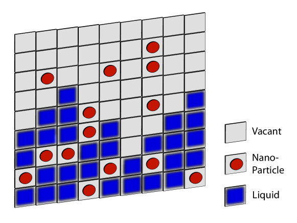
Figure 1: The sketch indicates how the substrate is divided into lattice sites and shows the three possible states of each lattice site.

We consider a simplified coarse-grained two-dimensional model for the system. The surface of the substrate is divided into a square array of discrete lattice sites. We choose the cell size so that each cell may be occupied by at most one nano-particle, i.e. the lattice spacing $\sigma$ is roughly equal to the diameter of the nano-particles. As a consequence, each lattice site must be in one of three possible states: (i) occupied by a nano-particle, (ii) occupied by liquid or (iii) unoccupied (as displayed in Fig. 1). To characterise the state of the system, we introduce two occupation numbers for each lattice site $i$: $n_{i}$ for nano-particles and $l_{i}$ for liquid. These occupation numbers are binary values which describe the state of each site. The occupation numbers for (i) a lattice site containing a nano-particle would be $n_{i}=1$, $l_{i}=0$, for (ii) a site occupied by a film of liquid we have $n_{i}=0$, $l_{i}=1$ and for (iii) a vacant site we have $n_{i}=0$, $l_{i}=0$. This type of lattice model has the following Hamiltonian [28]:

$$E = -\epsilon_{l}\sum_{<ij>}l_{i}l_{j}-\epsilon_{n}\sum_{<ij>}n_{i}n_{j}-\epsilon_{nl}\sum_{<ij>}n_{i}l_{j}$$ (1)

$$-\mu\sum_{i}l_{i}+\sum_{i}\phi_{i}^{l}l_{i}+\sum_{i}\phi_{i}^{n}n_{i}\hskip 5.69054pt,$$

where $\sum_{<ij>}$ denotes a sum over pairs of nearest neighbours. $\phi^{l}_{i}$ and $\phi^{n}_{i}$ are external potentials acting on the liquid and nano-particles respectively, at lattice site $i$. Three interaction terms are included which determine the strength of attraction between neighbouring cells. $\epsilon_{l}$ is the interaction energy between two adjacent cells containing films of liquid, $\epsilon_{n}$ is for adjacent cells which both contain nano-particles and $\epsilon_{nl}$ is the energy between a cell containing a nano-particle and a cell containing liquid. The amount of liquid on the surface is not a conserved quantity because it can evaporate to and condense from a reservoir of vapour above the surface. $\mu$ is the chemical potential of this reservoir.

From the Hamiltonian (1) we can derive an expression for the free energy of the system. The probability that a lattice site $i$ is covered by a liquid film in an equilibrium configuration is given by the following integral over time $t$:

$$\rho_{i}^{l}=\lim_{\tau\to\infty}\frac{1}{\tau}\int_{0}^{\tau}l_{i}(t)dt.$$ (2)

Similarly, the probability that a lattice site $i$ contains a nano-particle is given by the following expression:

$$\rho_{i}^{n}=\lim_{\tau\to\infty}\frac{1}{\tau}\int_{0}^{\tau}n_{i}(t)dt.$$ (3)

By choosing the grid spacing $\sigma$ to be our unit of length, equal to one, these probabilities are also equal to the local number densities for the liquid and nano-particles. Following the approach described in Refs. [43, 44], we make a Bragg-Williams mean field approximation for the (semi-grand) free energy of the system:

$$F = k_{B}T\sum_{i}[\rho_{i}^{l}\ln\rho_{i}^{l}+(1-\rho_{i}^{l})\ln(1-\rho_{i}^{l})+\rho_{i}^{n}\ln\rho_{i}^{n}$$ (4)

$$+(1-\rho_{i}^{n})\ln(1-\rho_{i}^{n})]-\epsilon_{l}\sum_{<ij>}\rho_{i}^{l}\rho_{j}^{l}-\epsilon_{n}\sum_{<ij>}\rho_{i}^{n}\rho_{j}^{n}$$

$$-\epsilon_{nl}\sum_{<ij>}\rho_{i}^{n}\rho_{j}^{l}-\mu\sum_{i}\rho_{i}^{l}+\sum_{i}\phi_{i}^{l}\rho_{i}^{l}+\sum_{i}\phi_{i}^{n}\rho_{i}^{n}\hskip 5.69054pt,$$

where $k_{B}$ is Boltzmann’s constant and T is the temperature. This is a semi-grand free energy because the liquid is treated in the grand canonical ensemble (the reservoir of vapour fixes the chemical potential $\mu$), whereas the number of nano-particles in the system is a conserved quantity (so these are treated canonically). Eq. (4) is derived using a ‘zeroth-order’ mean-field approximation and thus higher order terms are omitted (e.g. the terms involving $\ln(1-\rho_{i}^{n}-\rho_{i}^{l})$ which describe the excluded area correlations between the nano-particles and the liquid). If we assume that the density values only vary on length scales $\gg\sigma$, then we can define a gradient operator for this discrete system:

$$\nabla\rho^{l}_{x,y} \equiv \left(\rho^{l}_{x+1,y}-\rho^{l}_{x,y},\rho^{l}_{x,y+1}-\rho^{l}_{x,y}\right),$$

$$\nabla\rho^{n}_{x,y} \equiv \left(\rho^{n}_{x+1,y}-\rho^{n}_{x,y},\rho^{n}_{x,y+1}-\rho^{n}_{x,y}\right),$$ (5)

where each lattice site $i$ is now represented by the coordinates $(x,y)$. Using the operators (5) we can express the summation over pairs of nearest neighbours as

$$\sum_{<ij>}\rho_{i}^{\alpha}\rho_{j}^{\beta}=4\sum_{i}\rho_{i}^{\alpha}\rho_{i}^{\beta}-\sum_{i}(\nabla\rho_{i}^{\alpha})\cdot(\nabla\rho_{i}^{\beta}),$$ (6)

where $\alpha,\beta=n,l$. Substituting (6) into our lattice free energy (4) we obtain

$$F = k_{B}T\sum_{i}[\rho_{i}^{l}\ln\rho_{i}^{l}+(1-\rho_{i}^{l})\ln(1-\rho_{i}^{l})+\rho_{i}^{n}\ln\rho_{i}^{n}$$ (7)

$$+(1-\rho_{i}^{n})\ln(1-\rho_{i}^{n})]-\sum_{i}\bigg{[}\frac{4}{2}\epsilon_{l}(\rho_{i}^{l})^{2}+\frac{4}{2}\epsilon_{n}(\rho_{i}^{n})^{2}+4\epsilon_{nl}\rho_{i}^{n}\rho_{i}^{l}\bigg{]}$$

$$+\sum_{i}\bigg{[}\frac{\epsilon_{l}}{2}(\nabla\rho_{i}^{l})^{2}+\frac{\epsilon_{n}}{2}(\nabla\rho_{i}^{n})^{2}+\epsilon_{nl}(\nabla\rho_{i}^{n})\cdot(\nabla\rho_{i}^{l})\bigg{]}$$

$$-\mu\sum_{i}\rho_{i}^{l}+\sum_{i}\phi_{i}^{l}\rho_{i}^{l}+\sum_{i}\phi_{i}^{n}\rho_{i}^{n}\hskip 5.69054pt,$$

where the factor of $\frac{1}{2}$ is included to avoid double counting. Taking the continuum limit, so that $\sum_{i}\to\int d{\bf r}$, $\rho_{i}^{n}\to\rho_{n}({\bf r})$, $\rho_{i}^{l}\to\rho_{l}({\bf r})$, $\phi_{i}^{n}\to\phi_{n}({\bf r})$ and $\phi_{i}^{l}\to\phi_{l}({\bf r})$ where the vector ${\bf r}=(x,y)$ is a continuous variable, we obtain for the free energy of the system:

$$F[\rho_{l},\rho_{n}] = \int d{\bf r}\bigg{[}f(\rho_{l}({\bf r}),\rho_{n}({\bf r}))+\frac{\epsilon_{l}}{2}(\nabla\rho_{l}({\bf r}))^{2}$$ (8)

$$+\frac{\epsilon_{n}}{2}(\nabla\rho_{n}({\bf r}))^{2}+\epsilon_{nl}(\nabla\rho_{n}({\bf r}))\cdot(\nabla\rho_{l}({\bf r}))\bigg{]}$$

$$+\int d{\bf r}\rho_{l}({\bf r})(\phi_{l}({\bf r})-\mu)+\int d{\bf r}\rho_{n}({\bf r})\phi_{n}({\bf r}),$$

where

$$f(\rho_{l},\rho_{n}) = k_{B}T[\rho_{l}\ln\rho_{l}+(1-\rho_{l})\ln(1-\rho_{l})+\rho_{n}\ln\rho_{n}$$ (9)

$$+(1-\rho_{n})\ln(1-\rho_{n})]-2\epsilon_{l}\rho_{l}^{2}-2\epsilon_{n}\rho_{n}^{2}-4\epsilon_{nl}\rho_{n}\rho_{l}.$$

This free energy functional may be employed to determine the phase diagram of the system – i.e. the state of the system in the thermodynamic limit (see Section 4). However, the observed patterns are often non-equilibrium structures that are ‘dried in’, i.e., that evolve towards the equilibrium state on a time scale that is much longer than the typical observation times. To model the non-equilibrium processes that result in the observed self-organised structures, one needs kinetic equations for the time evolution of the densities. They are developed in the following section.

3 Modelling the Dynamics of the System

The chemical potential of the nano-particles may be calculated using the following functional derivative [45, 46, 47]:

$$\mu_{n}=\frac{\delta F[\rho_{n},\rho_{l}]}{\delta\rho_{n}}.$$ (10)

In equilibrium systems the chemical potentials take a uniform value throughout the system. However, this is not the case for non-equilibrium configurations that the system takes during its time evolution. There, the chemical potential varies temporally and spatially over the surface. In particular, non-equilibrium density profiles $\rho_{l}({\bf r},t)$ and $\rho_{n}({\bf r},t)$ give, via Eq. (10), a non-equilibrium chemical potential for the nano-particles $\mu_{n}({\bf r},t)$. Thus, the time-dependent densities are coarse-grained ‘average’ quantities. Assuming that locally, the system is in equilibrium, we may define these non-equilibrium density fields in a similar way as the equilibrium densities [see Eqs. (2) and (3)]:

$$\rho_{i}^{l} = \frac{1}{\tau_{M}}\int_{0}^{\tau_{M}}l_{i}(t)dt,$$ (11)

$$\rho_{i}^{n} = \frac{1}{\tau_{M}}\int_{0}^{\tau_{M}}n_{i}(t)dt,$$ (12)

where $\tau_{M}$ is now a finite time that is large compared to the solvent molecular collision time, but is small compared to the time scale for a nano-particle to move from one lattice site to a neighbouring lattice site. If we now assume that the driving force which causes a flux of the nano-particles over the surface of the substrate to be given by the gradient of the chemical potential $\mu_{n}$, then the nano-particle current is given by

$${\bf{j}}_{n}=-M_{n}({\bf r},t)\nabla\frac{\delta F[\rho_{n},\rho_{l}]}{\delta\rho_{n}({\bf r},t)},$$ (13)

where $M_{n}({\bf r},t)$ is a mobility coefficient which we assume to depend on the local densities $\rho_{n}({\bf r},t)$ and $\rho_{l}({\bf r},t)$. Since the number of nano-particles in the system is conserved we can combine Eq. (13) with the continuity equation to get

$$\frac{\partial\rho_{n}({\bf r},t)}{\partial t}=\nabla\cdot\left[M_{n}(\rho_{n},\rho_{l})\nabla\frac{\delta F[\rho_{n},\rho_{l}]}{\delta\rho_{n}({\bf r},t)}\right].$$ (14)

We expect that when the liquid density is uniform throughout the system ($\rho_{l}({\bf r})=\rho$) and the density of the nano-particles is small everywhere ($\rho_{n}({\bf r})\ll 1$) then the nano-particle dynamics given by Eq. (14) must reduce to the diffusion equation (i.e. Eq. (13) becomes Fick’s law). When we apply this to Eq. (10), for small $\rho_{n}$, we get the leading order term:

$$\mu_{n}({\bf r})\approx k_{B}T\ln\rho_{n}({\bf r})+C+O(\rho_{n}),$$ (15)

where $C=C(\rho_{l})$ represents constant terms. Substituting Eq. (15) into Eq. (14) we see that in order for Eq. (14) to reduce to the diffusion equation the mobility $M_{n}$ has to be proportional to $\rho_{n}({\bf r},t)$. Therefore, we write the nano-particle mobility as:

$$M_{n}=\rho_{n}({\bf r},t)m(\rho_{l}({\bf r},t)),$$ (16)

where $m(\rho_{l}({\bf r},t))$ is a function of the local liquid density. We assume that the diffusion of the nano-particles over the surface is caused by the Brownian ‘kicks’ from the molecules in the liquid. Therefore when the liquid density is low (on the dry substrate) the nano-particles are almost immobile. However, when the density of the liquid on the surface is high (where the substrate is covered by the liquid film), the nano-particles are much more mobile. We model this behaviour by a function $m(\rho_{l}({\bf r},t))$ which switches between a very small value, when $\rho_{l}$ is small and $\alpha$, which is the mobility coefficient for the nano-particles in a liquid film, when $\rho_{l}>0.5$. The precise form of $m(\rho_{l})$ has a negligible effect on the qualitative behaviour of the system. Here we use

$$m(\rho_{l})=\frac{\alpha}{2}\{1+\tanh[30(\rho_{l}-\frac{1}{2})]\}.$$ (17)

Next we consider the time evolution of the liquid density $\rho_{l}({\bf r},t)$. The dominant process governing the dynamics of the liquid is the evaporation and condensation of the liquid between the surface and the vapour reservoir above the substrate. We define two different chemical potentials: $\mu$ is the chemical potential of the liquid in the reservoir (cf. Eq. (4)) and $\mu_{S}({\bf r},t)=\frac{\delta F}{\delta\rho_{l}}+\mu$ denotes the local chemical potential of the liquid on the substrate. We assume that the evaporative contribution to the time evolution of the liquid density is proportional to the difference between $\mu_{S}({\bf r},t)$ and $\mu$. This gives us the following expression:

$$\frac{\partial\rho_{l}({\bf r},t)}{\partial t}=-M_{l}^{nc}\frac{\delta F[\rho_{n},\rho_{l}]}{\delta\rho_{l}({\bf r},t)},$$ (18)

where the dynamical coefficient $M_{l}^{nc}$ is assumed to be a constant. The value of $M_{l}^{nc}$ determines the rate of the non-conserved (evaporation) dynamics of the liquid. We should also allow for (conserved) diffusive motion of the liquid over the surface. We assume from DDFT that the diffusion of the liquid takes a similar form as the diffusion of the nano-particles given in Eq. (14). We therefore model the full liquid dynamics by combining the diffusive and the evaporative terms

$$\frac{\partial\rho_{l}({\bf r},t)}{\partial t}=\nabla\cdot\left[M_{l}^{c}\rho_{l}\nabla\frac{\delta F[\rho_{n},\rho_{l}]}{\delta\rho_{l}({\bf r},t)}\right]-M_{l}^{nc}\frac{\delta F[\rho_{n},\rho_{l}]}{\delta\rho_{l}({\bf r},t)}.$$ (19)

The mobility coefficient $M_{l}^{c}$ for the conserved part of the dynamics is assumed to be constant. The ratio between the conserved and non-conserved mobility coefficients determines the influence that the diffusive/evaporative terms have on the overall dynamics of the liquid (i.e. $M_{l}^{nc}/M_{l}^{c}\gg 1$ corresponds to the case when the liquid dynamics are strongly dominated by evaporation and $M_{l}^{nc}/M_{l}^{c}\ll 1$ corresponds to the case when liquid diffusion plays an important role in the dynamics). Thus, equations (8), (9), (14) and (19), taken together, define our model equations, which govern the dynamics of the system.

Note that when the liquid density $\rho_{l}({\bf r},t)$ is a constant, the theory reduces to the DDFT developed by Marconi and Tarazona [39], that may be obtained by approximating the Fokker-Planck equation for a system of Brownian particles with overdamped stochastic equations of motion [39, 40, 41, 42, 43]. Equations similar to (19) can also be derived in the context of hydrodynamics. The resulting mesoscopic hydrodynamic thin film equations contain different mobilities and local energies [48, 49]. The combination of the diffusive and the evaporative terms can also be seen as a combination of a conserved Cahn-Hillard-type dynamics with a non-conserved Allen-Cahn-type dynamics [50, 51, 52].

4 Phase Behaviour

4.1 One-component fluid

It is important to understand the equilibrium behaviour of the fluid in our system as this gives us some insight into how the system behaves when it is out of equilibrium. Of particular importance is to determine what phases we may observe and the stability of these phases. Since we are modelling the evaporative dewetting of the liquid we initially seek parameter values which lead to a high density liquid phase (liquid film) coexisting with a low density phase (‘dry’ substrate). Employing a linear stability analysis, we calculate the spinodal curve, i.e., the limit of linear stability for an infinitely extended system. The spinodal curve is defined as the locus of points where the curvature of the free energy is zero, $\frac{d^{2}F}{d\rho^{2}}=0$, which is equivalent to the isothermal compressibility being zero [45]. Note that in this section we set $\rho_{l}=\rho$, for simplicity. We also calculate the binodal curve, i.e., the coexisting density values for a system in equilibrium, by equating the chemical potentials, temperature and pressure in each of the coexisting phases. The area outside the binodal curve is a stable region where we see no phase separation. Inside the binodal curve we have phase separation in the thermodynamic limit. However, the linear stability of the fluid depends on whether the curvature of free energy is positive or negative. When we have positive curvature (outside the spinodal curve), the system at this state point rests within a local minimum of the free energy, i.e., it is linearly but not absolutely stable. There is a free energy barrier that must be traversed to cross into the (absolutely stable) equilibrium phase. This is known as the metastable region, where local fluctuations in the density (if sufficient in size) create nucleation points for the phase transition to occur. When the curvature of the free energy is negative (inside the spinodal curve) there is no free energy barrier. This is the unstable region where we have spontaneous phase separation, i.e. where fluctuations in the densities spontaneously grow. One may also say that the homogenous fluid layer is linearly unstable to harmonic perturbations with certain wave numbers.

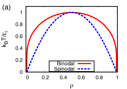
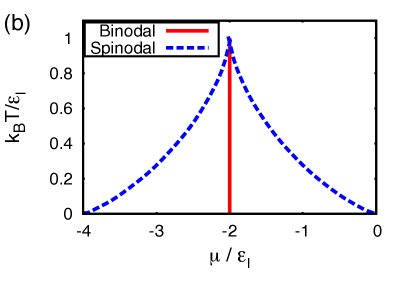
Figure 2: Phase diagrams showing the binodal (solid line) and spinodal (dotted line) for the one component pure fluid. In (a) we plot the phase diagram in the temperature $T$ versus density $\rho$ plane and in (b) we display the same phase diagram in the temperature versus chemical potential $\mu$ plane.

We first consider the phase behaviour of the reduced case where we have a single component fluid with no nano-particles (i.e. $\rho_{n}=0$), as shown in Fig. 2. We set the external potential $\phi_{l}({\bf r})=0$ which results in a uniform fluid density $\rho_{l}({\bf r})=\rho=\frac{N}{A}$, where N is the number of ‘particles’ of liquid (i.e. filled lattice sites) and A is the area of the system. From Eq. (9) we find that the Helmholtz free energy per unit area of the uniform system is

$$f=\frac{F}{A}=k_{B}T\left[\rho\ln\rho+(1-\rho)\ln(1-\rho)\right]-2\epsilon_{l}\rho^{2}.$$ (20)

We define the Helmholtz free energy per ‘particle’ as

$$a\equiv\frac{F}{N}=k_{B}T\left[\ln\rho+\frac{(1-\rho)}{\rho}\ln(1-\rho)\right]-2\epsilon_{l}\rho.$$ (21)

From this, we may calculate other thermodynamic quantities: the pressure $P$ and chemical potential $\mu$, which are given by the following relations [45]:

$$P = \rho^{2}\left(\frac{\partial a}{\partial\rho}\right),$$ (22)

$$\mu = a+\rho\left(\frac{\partial a}{\partial\rho}\right).$$ (23)

We can calculate the spinodal for the one component fluid from the free energy Eq. (20) and the definition of the spinodal $\frac{d^{2}f}{d\rho^{2}}=0$, giving us the following equation:

$$\frac{k_{B}T}{\epsilon_{l}}=4\rho(1-\rho).$$ (24)

Equations (21) and (22) give the following expression for the pressure in the system:

$$P=-k_{B}T\ln(1-\rho)-2\epsilon_{l}\rho^{2}.$$ (25)

In order to simplify the task of determining the phase diagram, we may use the symmetry of the Hamiltonian (1). The Hamiltonian remains unchanged under the exchange $l_{i}\to(1-l_{i})$, i.e., it has a symmetry between ‘holes’ (nearly dry substrate) and ‘drops’ (liquid layer). This means that for the one component fluid, the phase diagram is symmetric around the line $\rho=\frac{1}{2}$, i.e. for a phase on the binodal with a density of $\rho=\rho_{1}$ the coexisting phase has a density of $\rho_{2}=(1-\rho_{1})$. Using Eq. (25) and this symmetry of the Hamiltonian, we obtain the following expression for the density along the binodal, by equating the pressure in the two phases ($P_{1}=P_{2})$:

$$\frac{k_{B}T}{\epsilon_{l}}=\frac{2(2\rho-1)}{\ln[\rho/(1-\rho)]}$$ (26)

The maximum on this curve is at $\rho=\frac{1}{2}$ and corresponds to the critical temperature $k_{B}T/\epsilon_{l}=1$. Below the critical temperature there are two solutions; these are the coexisting densities. The binodal and spinodal curves for the pure liquid are plotted in Fig. 2(a). Fig. 2(b) shows the value of the chemical potential along these curves.

The spinodal region can also be calculated from the dynamical equations (14) and (19) employing a linear stability analysis. This allows us to determine the typical length scales of the density fluctuations in the liquid film which might exist during the evaporation process. To perform the linear stability analysis we consider a liquid density which varies in space and time $\rho_{l}=\rho({\bf r},t)$. The free energy for the single component fluid ($\rho_{n}=0$) is given by:

$$F=\int d{\bf r}\bigg{[}f(\rho)+\frac{\epsilon}{2}(\nabla\rho)^{2}-\mu\rho\bigg{]},$$ (27)

where the subscript on the liquid interaction variable $\epsilon_{l}$ is dropped for simplicity. The steady state solutions of the liquid dynamical equation Eq. (19) represent the equilibrium density configurations. There are several steady states for this system, (e.g. a density profile containing a free interface between two co-existing densities with $\mu=\mu_{\mathrm{coex}}$) but here we consider the simplest steady state: a flat homogeneous film with a density $\rho=\rho_{0}$ which is defined by:

$$\frac{\delta F}{\delta\rho}\bigg{|}_{\rho_{0}}=0.$$ (28)

We consider small amplitude perturbations $\delta\rho$ from $\rho_{0}$ of the form $\rho=\rho_{0}+\delta\rho=\rho_{0}+\phi e^{i{\bf k\cdot r}}e^{\beta t}$, where the amplitude $\phi\ll 1$ is a small positive constant, $k=|{\bf k}|$ is the wave number and $\beta$ is the rate of growth/decay with time (for positive/negative values) of the perturbation. We substitute this expression for $\rho$ into the dynamical equation (19) and expand in powers of $\delta\rho$. Then taking just the leading order terms allows us to derive a simple expression for $\beta$ which can be solved analytically.

A Taylor series expansion of the functional derivative of the free energy (27) yields:

$$\frac{\delta F}{\delta\rho} = \frac{\partial f}{\partial\rho}-\epsilon\nabla^{2}\rho-\mu$$ (29)

$$= \frac{\partial f}{\partial\rho}\bigg{|}_{\rho_{0}}+\frac{\partial^{2}f}{\partial\rho^{2}}\bigg{|}_{\rho_{0}}\delta\rho+\epsilon k^{2}\delta\rho-\mu+O(\delta\rho^{2}).$$

Substituting this approximation for the functional derivative (29) into the dynamical equation (19) we obtain

$$\beta\delta\rho = M_{c}\nabla\cdot\bigg{[}\rho_{0}(ik\frac{\partial^{2}f}{\partial\rho^{2}}\bigg{|}_{\rho_{0}}\delta\rho+i\epsilon k^{3}\delta\rho)\bigg{]}-$$ (30)

$$M_{nc}\bigg{(}\frac{\partial f}{\partial\rho}\bigg{|}_{\rho_{0}}+\frac{\partial^{2}f}{\partial\rho^{2}}\bigg{|}_{\rho_{0}}\delta\rho+\epsilon k^{2}\delta\rho-\mu\bigg{)}+O(\delta\rho^{2}).$$

Using the definition of $\rho_{0}$ [Eq. (28)] gives $\frac{\partial f}{\partial\rho}\big{|}_{\rho_{0}}-\mu=0$ and neglecting second order terms $O(\delta\rho^{2})$ we arrive at the expression for the growth rate

$$\beta=-\bigg{(}M_{c}\rho_{0}k^{2}+M_{nc}\bigg{)}\bigg{(}\frac{\partial^{2}f}{\partial\rho^{2}}\bigg{|}_{\rho_{0}}+\epsilon k^{2}\bigg{)}.$$ (31)

When $\beta$ is positive, small perturbations from the steady state $\rho_{0}$ with the wave number $k$ grow in amplitude over time. Conversely, if $\beta$ is negative then small perturbations decay. Since $M_{c}$, $\rho_{0}$, $k^{2}$, $M_{nc}$ and $\epsilon$ are all positive quantities, $\beta$ is always negative (i.e. the fluid is stable for all wave numbers $k$) when the second derivative $\frac{\partial^{2}f}{\partial\rho^{2}}\big{|}_{\rho_{0}}$ is positive. However when $\frac{\partial^{2}f}{\partial\rho^{2}}\big{|}_{\rho_{0}}$ is negative, we find that $\beta$ is positive for small values of $k$ and negative when $k$ is large - i.e. the fluid is unstable against long wavelength (small wave number) fluctuations in density. This corresponds to the thermodynamic definition of the spinodal as previously discussed. We may define a critical wave number $k_{c}$, as the wave number at which $\beta(k_{c})=0$. When $M_{nc}\neq 0$ and $\frac{\partial^{2}f}{\partial\rho^{2}}\big{|}_{\rho_{0}}<0$, the critical wave number $k_{c}$ is given by:

$$k_{c}=\pm\sqrt{-\frac{1}{\epsilon}\frac{\partial^{2}f}{\partial\rho^{2}}\bigg{|}_{\rho_{0}}}.$$ (32)

The real system we are modelling is very large ($L\gg 2\pi/k_{c}$), which means fluctuations can occur on the full spectrum of wave numbers. The mode with wave number $k=k_{m}$, which has the largest positive value for $\beta$ grow the fastest. The wave number $k_{m}$ corresponds to a typical length scale $2\pi/k_{m}$ that are visible during the early stages of spinodal decomposition. However, at later stages (beyond the linear stage) the length scale of the modulations is likely to deviate from this value as the pattern coarsens. For the purely evaporative case when $M_{c}=0$, the maximum value of $\beta(k)$ occurs at $k=k_{m}=0$, which means there is no typical length scale in the early stages of the evaporation process. However, in the purely diffusive case $M_{nc}=0$ (and $\frac{\partial^{2}f}{\partial\rho^{2}}\big{|}_{\rho_{0}}<0$), $\beta(k=0)=0$ due to mass conservation, and the maximum value of $\beta(k)$ occurs at a non-zero value of $k_{m}$, so the typical length scale $2\pi/k_{m}$ is visible during the spinodal decomposition–evaporation. In all other cases the following expression is both a necessary and sufficient condition for the existence of the typical length scale (i.e. $k_{m}\neq 0$):

$$\frac{M_{nc}}{M_{c}}<-\frac{\rho_{0}}{\epsilon}\frac{\partial^{2}f}{\partial\rho^{2}}\bigg{|}_{\rho_{0}}.$$ (33)

If a typical length scale does exist, then the corresponding wave number $k_{m}$ is given by:

$$k_{m}=\sqrt{-\frac{1}{2}\bigg{(}\frac{1}{\epsilon}\frac{\partial^{2}f}{\partial\rho^{2}}\bigg{|}_{\rho_{0}}+\frac{M_{nc}}{\rho_{0}M_{c}}\bigg{)}}.$$ (34)

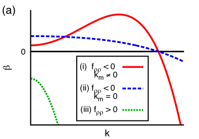
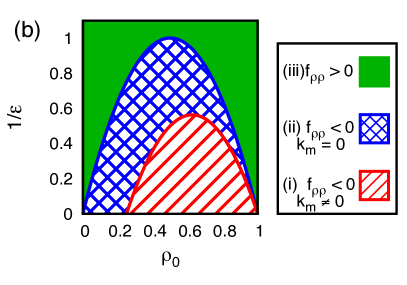
Figure 3: There are three possible forms for $\beta(k)$: (a) shows an example of each form and (b) shows the regions in parameter space where these different types of $\beta(k)$ curves occur, for the case when $M_{nc}/M_{c}=1$ and $k_{B}T=1$.

Figure 3 displays (a) typical $\beta(k)$ curves for a one-component fluid and (b) the values of $1/\epsilon$ and $\rho_{0}$ where each type of curve is found (for the case when $M_{nc}/M_{c}=1$ and $k_{B}T=1$). Three distinct cases are displayed: Case (i) the solid line (red online) in (a) and the striped area (red online) in (b) display the case when one observes the growth of density fluctuations with a typical length scale. Case (ii), the dashed line (blue online) in (a) and the hashed area (blue online) in (b) correspond to the situation when the fluid is unstable for density fluctuations corresponding to small wave numbers $k$ but no typical length scale is observed, because the fastest growing mode is the $k=0$ fluctuation. Case (iii), the dotted line (green online) in (a), corresponding to the (green) solid area in (b), displays the situation when the liquid is linearly stable against density fluctuations with all wave numbers $k$.

4.2 Binary mixture

To determine the binodal and spinodal curves for the binary mixture is more challenging than for the one component system. There are many more parameters defining the model. In particular, the behaviour of the system strongly depends on the ratios between the different interaction strengths $\epsilon_{l}$, $\epsilon_{n}$ and $\epsilon_{nl}$. Ref. [53] gives a good overview of the equilibrium bulk fluid phase behaviour for binary fluid mixtures and the different classes of phase diagrams that may be observed. Here, we only describe the influence of the chemical potential of the nano-particles $\mu_{n}$ on the densities in the coexisting phases and on the critical point.

For two phases of a binary mixture to coexist in thermodynamic equilibrium, there are four conditions that must be satisfied. We denote these two phases as (i) the low density phase (LDP) or ‘dry’ substrate and (ii) the high density phase (HDP) or substrate covered by a colloidal film:

$$T^{LDP}=T^{HDP},$$ (35)

$$\mu_{l}^{LDP}=\mu_{l}^{HDP},$$ (36)

$$\mu_{n}^{LDP}=\mu_{n}^{HDP},$$ (37)

$$P^{LDP}=P^{HDP},$$ (38)

where $T$ is the temperature, $\mu_{l}$ and $\mu_{n}$ are the chemical potentials of the liquid and nano-particles respectively, $P$ is the pressure and the superscript denotes the phase. The first of these equations is trivial to satisfy in our model. We may then fix the chemical potential of the nano-particles, to some value $\eta$, and then solve equations (36), (38), $\mu_{n}^{LDP}=\eta$ and $\mu_{n}^{HDP}=\eta$ for the four density values: $\rho_{l}^{LDP}$, $\rho_{n}^{LDP}$, $\rho_{l}^{HDP}$ and $\rho_{n}^{HDP}$. The curves of the coexisting density values (binodals) for the parameters $\epsilon_{nl}/\epsilon_{l}=0.57$ and $\epsilon_{n}=0.43$ are displayed in Fig. 4. The density values calculated for the two phases meet at a critical temperature to form binodal curves similar to the one found for the one component system Fig. 2a. However, we find that the reflection symmetry w.r.t. the liquid density $\rho_{l}=1/2$ seen for the one component fluid is broken. In particular, the critical point of the liquid is no longer at $\rho_{l}=1/2$. The liquid binodal reduces to the one for the pure liquid as $\mu_{n}\to\pm\infty$. The curves for $\mu_{n}\to-\infty$ and $\mu_{n}\to\infty$ are identical within our model due to the symmetry of the Hamiltonian (1). We observe that the density of the nano-particles $\rho_{n}\to 0$ becomes very small as the chemical potential decreases $\mu_{n}\to-\infty$. Conversely, the density becomes very large $\rho_{n}\to 1$ as the chemical potential increases $\mu_{n}\to\infty$. The critical point on the nano-particle binodal curve shifts in a similar manner to that of the liquid binodal.

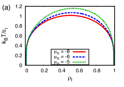
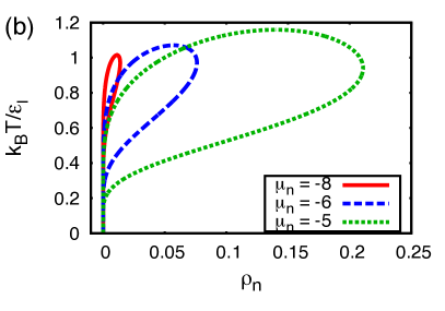
Figure 4: Binodal curves for the binary mixture for varying fixed values of the chemical potential of the nano-particles $\mu_{n}$, for the case when $\epsilon_{n}/\epsilon_{l}=0.43$ and $\epsilon_{nl}/\epsilon_{l}=0.57$.

We now consider the linear stability of the fluid for the two component case. There are many different possible steady states for the binary system including some with interfaces between coexisting phases. However, here we limit ourselves to investigating the linear stability of the simplest steady state: where both components have a uniform constant density over the surface. The uniform density of the nano-particle film is denoted by $\rho_{n}=\rho_{n}^{0}$ and the density of the liquid is given by $\rho_{l}=\rho_{l}^{0}$ where $\rho_{l}^{0}$ is determined from the condition:

$$\frac{\delta F}{\delta\rho_{l}}\bigg{|}_{\rho_{l}^{0}}=0.$$ (39)

We consider small amplitude perturbations in the density of both components from this steady state. We assume these perturbations to take the form:

$$\rho_{l}=\rho_{l}^{0}+\delta\rho=\rho_{l}^{0}+\phi e^{i{\bf k\cdot r}}e^{\beta t},$$ (40)

$$\rho_{n}=\rho_{n}^{0}+\chi\delta\rho=\rho_{n}^{0}+\chi\phi e^{i{\bf k\cdot r}}e^{\beta t},$$ (41)

where the amplitude $|\phi|\ll 1$ and the parameter $\chi$ is the ratio between the perturbation in the densities of the two components. The sign of $\chi$ determines whether any instabilities are in-phase (positive) or anti-phase (negative) between the two coupled density fields. From the magnitude of $\chi$ we can determine whether an instability is driven by the liquid component ($|\chi|\ll 1$), the nano-particles ($|\chi|\gg 1$) or stems from the interaction between the two components ($|\chi|=O(1)$). Making a Taylor series expansion of the functional derivative of the free energy with respect to the liquid density $\frac{\delta F}{\delta\rho_{l}}$, keeping only terms linear in $\delta\rho$ and substituting this expression into the liquid dynamical equation (19) we obtain

$$\beta=-(M^{l}_{c}\rho_{l}^{0}k^{2}+M^{l}_{nc})\bigg{(}\frac{\partial^{2}f}{\partial\rho_{l}^{2}}\bigg{|}_{\rho_{l}^{0},\rho_{n}^{0}}+\chi\frac{\partial^{2}f}{\partial\rho_{l}\partial\rho_{n}}\bigg{|}_{\rho_{l}^{0},\rho_{n}^{0}}+k^{2}\epsilon_{l}+k^{2}\chi\epsilon_{nl}\bigg{)}.$$ (42)

Turning our attention now to the nano-particles: in order to linearise Eq. (14), we must first examine the nano-particle mobility function $M^{n}(\rho_{l},\rho_{n})=\rho_{n}m(\rho_{l})$, given by Eqs. (16) and (17) in our model. Making a Taylor series expansion of the function $m(\rho_{l})$ we obtain

$$\frac{m}{\alpha}=\hskip 2.27621pt\gamma_{0}+\gamma_{1}\delta\rho+O(\delta\rho^{2}),$$ (43)

where $\gamma_{0}\approx 0$ for small values of $\rho_{l}$ ($\rho_{l}<0.45$) and $\gamma_{0}\approx 1$ for large values of $\rho_{l}$ ($\rho_{l}>0.55$). Substituting a Taylor series expansion of the functional derivative, together with Eq. (43), into the time evolution equation for the nano-particles Eq. (14) we find

$$\chi\beta=-\alpha\rho_{n}^{0}\gamma_{0}k^{2}\bigg{(}\chi\frac{\partial^{2}f}{\partial\rho_{n}^{2}}\bigg{|}_{\rho_{l}^{0},\rho_{n}^{0}}+\frac{\partial^{2}f}{\partial\rho_{n}\partial\rho_{l}}\bigg{|}_{\rho_{l}^{0},\rho_{n}^{0}}+k^{2}\chi\epsilon_{n}+k^{2}\epsilon_{l}\bigg{)}.$$ (44)

When $\rho_{l}$ is small, $\gamma_{0}\approx 0$. In consequence, $\chi=0$ and the Eqs. (42) and (44) reduce to the one of the one-component fluid (with a local free energy that depends also on $\rho_{n}^{0}$). We now address the case when $\rho_{l}>0.55$, and we therefore assume $\gamma_{0}=1$. The expressions for the time dependency of the amplitudes of the two density fields (Eq. (42) and Eq. (44)) can be solved simultaneously to determine $\beta$ and $\chi$ as a function of the wave number $k$. This allows us to determine the stability of the fluid for different values of the system parameters. A fact that simplifies the analysis is that these two equations may be written in matrix form (similar to the case of two coupled mesoscopic hydrodynamic equations for dewetting two-layer films [54]):

$$\beta\left(\begin{array}[]{c}\chi\\ 1\end{array}\right)=\mathbf{M}\cdot\mathbf{G}\left(\begin{array}[]{c}\chi\\ 1\end{array}\right),$$ (45)

where,

$$\mathbf{M} = \left(\begin{array}[]{cc}-\alpha\rho_{n}^{0}k^{2}&\hskip 14.22636pt0\\ 0&-(M^{l}_{c}\rho_{l}^{0}k^{2}+M^{l}_{nc})\end{array}\right),$$ (48)

$$\mathbf{G} = \left(\begin{array}[]{cc}k^{2}\epsilon_{n}+f_{nn}&k^{2}\epsilon_{nl}+f_{nl}\\ k^{2}\epsilon_{nl}+f_{nl}&k^{2}\epsilon_{l}+f_{ll}\end{array}\right),$$ (51)

and we have used the shorthand notation $f_{ij}\equiv\frac{\partial^{2}f}{\partial\rho_{i}\partial\rho_{j}}\big{|}_{\rho_{l}^{0}\rho_{n}^{0}}$, where $i,j=n,l$ and where $n$ denotes the nano-particles and $l$ denotes the liquid. We can determine $\beta(k)$ using the following expression for the eigenvalues of a $2\times 2$ matrix:

$$\beta(k)=\frac{\mbox{Tr}(\mathbf{M\cdot G})}{2}\pm\sqrt{\frac{\mbox{Tr}(\mathbf{M\cdot G})^{2}}{4}-|\mathbf{M\cdot G}|}.$$ (52)

We define critical wave numbers $k=k_{c}$ for the density fluctuations in the two-component fluid as the wave numbers at which one of the two solutions of Eq. (52) is equal to zero. Below [Eqs. (55) and (56)] we derive explicit expressions for $k_{c}$ which can be used to determine the conditions for the linear stability of the two component fluid (i.e. the fluid is stable when there is no solution for $k_{c}$ and the function $\beta(k)<0$ for all wave numbers $k$). Since the matrix $\mathbf{M}$ is diagonal and all diagonal elements are non-zero the inverse $\mathbf{M^{-1}}$ exists, allowing us to rewrite Eq. (45) as a generalised eigenvalue problem

$$(\mathbf{G}-\mathbf{M^{-1}}\beta)\left(\begin{array}[]{c}\chi\\ 1\end{array}\right)=0.$$ (53)

Setting $\beta=0$ in this equation in order to find the critical wave numbers $k_{c}$, we find that the determinant $|\mathbf{G}|=0$, implying that

$$k_{c}^{4}(\epsilon_{n}\epsilon_{l}-\epsilon_{nl}^{2})+k_{c}^{2}(\epsilon_{n}f_{ll}+\epsilon_{l}f_{nn}-2\epsilon_{nl}f_{nl})+f_{nn}f_{ll}-f_{nl}^{2}=0.$$ (54)

In the special case when $\epsilon_{n}\epsilon_{l}=\epsilon_{nl}^{2}$, the critical wave number is given by:

$$k_{c}=\sqrt{\frac{f_{nl}^{2}-f_{nn}f_{ll}}{\epsilon_{n}f_{ll}+\epsilon_{l}f_{nn}-2\epsilon_{nl}f_{nl}}}.$$ (55)

However, more generally, when $\epsilon_{n}\epsilon_{l}\neq\epsilon_{nl}^{2}$, we have

$$k_{c}=\sqrt{\frac{-b\pm\sqrt{b^{2}-4ac}}{2a}},$$ (56)

where

$$a = \epsilon_{n}\epsilon_{l}-\epsilon_{nl}^{2},$$

$$b = \epsilon_{n}f_{ll}+\epsilon_{l}f_{nn}-2\epsilon_{nl}f_{nl},$$

$$c = f_{nn}f_{ll}-f_{nl}^{2}.$$ (57)

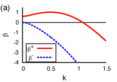
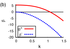
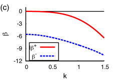
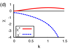
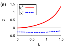
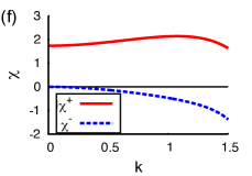
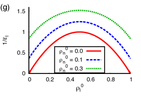
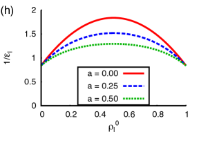
Figure 5: (a) - (f) Dispersion relations for the case when $\epsilon_{n}\epsilon_{l}>\epsilon_{nl}^{2}$,   $\epsilon_{n}f_{ll}+\epsilon_{l}f_{nn}-2\epsilon_{nl}f_{nl}>0$ (i.e. in Eq. (57) $a>0,b>0$) and $k_{B}T=1$. The graphs in the top row show $\beta(k)$ and the graphs in the middle row show $\chi(k)$. In (a) and (d) the parameters are: $\rho_{l}^{0}=0.648,\rho_{n}^{0}=0.3,\epsilon_{l}=1.25,\epsilon_{n}=0.5,\epsilon_{nl}=0.6,\mu=-3.35,M^{n}=1,M^{l}_{c}=0\mbox{ and }M^{l}_{nc}=1.$ In (b) and (e) the parameters are: $\rho_{l}^{0}=0.648,\rho_{n}^{0}=0.3,\epsilon_{l}=1.25,\epsilon_{n}=0.5,\epsilon_{nl}=0.6,\mu=-3.35,M^{n}=1,M^{l}_{c}=0\mbox{ and }M^{l}_{nc}=9$. In (c) and (f) the parameters are: $\rho_{l}^{0}=0.901,\rho_{n}^{0}=0.3,\epsilon_{l}=1.4,\epsilon_{n}=0.6,\epsilon_{nl}=0.8,\mu=-3.8,M^{n}=1,M^{l}_{c}=0\mbox{ and }M^{l}_{nc}=1.$ (g) shows how the spinodal line shifts for increasing $\rho_{n}^{0}$, where $\epsilon_{n}\epsilon_{l}-\epsilon_{nl}^{2}=0.25$, $\epsilon_{n}=\epsilon_{l}$ and $k_{B}T=1$. (h) shows how the spinodal line shifts as the value of $a=\epsilon_{n}\epsilon_{l}-\epsilon_{nl}^{2}$ increases, when $\rho_{n}^{0}=0.3$, $\epsilon_{n}=\epsilon_{l}$ and $k_{B}T=1$.

Note that the locus $c=0$ is the spinodal curve [55, 56]. We categorise the linear behaviour of the system by the signs of $a$ and $b$ in Eq. (57) as they have a profound impact on the shape of the dispersion curves. In Fig. 5 we display for the case when $a>0$ and $b>0$ all the different possible $\beta(k)$ curves, together with the corresponding $\chi(k)$. From Eq. (52) we see that there are two branches for $\beta(k)$, which we denote $\beta^{+}(k)$ and $\beta^{-}(k)$. The corresponding $\chi(k)$ curves are denoted $\chi^{+}$ and $\chi^{-}$, respectively. The $\beta^{+}$ branch (red solid lines in Fig. 5(a) - (c)) corresponds to the second term in Eq. (52) being positive and the $\beta^{-}$ branch (dashed lines) corresponds to the second term being negative. Due to mass conservation of the nano-particles, there is always one $\beta(k)$ branch that is zero at $k=0$, and $\chi=0$ at $k=0$ for the curve that corresponds to the $\beta(k)$ that is not zero at $k=0$. If $f_{ll}\geq 0$ then $\beta^{+}(k=0)=0$ and $\chi^{-}(k=0)=0$. Alternatively, if $f_{ll}\leq 0$ then $\beta^{-}(k=0)=0$ and $\chi^{+}(k=0)=0$.

Inspecting Fig. 5, we find that there are three possible forms for $\beta(k)$, similar to the one component fluid case (Fig. 3). In Fig 5(a) there is a maximum in $\beta^{+}$ at $k\neq 0$. This indicates that the fluid is unstable and that one will observe the growth of density fluctuations with a typical length scale $2\pi/k_{m}^{+}$ during the early stages of the spinodal process. Here $k_{m}^{+}$ refers to the wave number at the maximum of $\beta^{+}$. In the second case [Fig. 5(b)] the fluid is linearly unstable for density fluctuations with small wave numbers $k$ as in Fig. 5(a), but the maximum in $\beta^{+}(k)$ occurs at $k_{m}^{+}=0$, i.e. there is no typical length scale visible in the density profiles. In the last case, shown in Fig. 5(c), the fluid is stable for all wave numbers $k$. We can use Eq. (56) for the critical wave number $k_{c}$ to determine the stability of the system. Since $a>0$ and $b>0$ we observe that there is at most one positive root of $\beta(k)$, which only exists if $c<0$ (i.e. inside the spinodal). The spinodal curve when $a>0$ and $b>0$ is plotted in Fig. 5(g) and (h). In (g) we show how the spinodal line moves upwards in $1/\epsilon_{l}$ as the nano-particle density $\rho_{n}^{0}$ is increased. In (h) we show how the shape of the spinodal changes as the value of the parameter $a$ is increased. We find that larger values of $a$ make the spinodal curve flatter.

In the reduced case when $a=0$, one can determine from Eqs. (57) that $b$ is always be positive. We find the same three types of dispersion relations for this reduced case as we do for the $a>0$, $b>0$ case. For the case when $a>0$ and $b<0$ we observe that the fluid is unstable for all possible combinations of parameter values. When we have $a<0$ (where at least one of the components of the mixture is more attracted to the other component than to itself), we find that $b$ must be positive. In this regime, we observe that as $k\to\infty,\beta^{+}(k)\to\infty$ and $\beta^{-}(k)\to-\infty$. This indicates that the density fluctuations with an infinitesimally small typical length scale will grow fastest. This behaviour corresponds to a mixture that exhibits micro-phase separation. This behaviour is common in block copolymer systems, where chemical bonding prevents macroscopic demixing and instead demixing on the nano-scale is witnessed [57, 58]. Micro-phase separation is also observed in certain colloidal suspensions [59, 60, 61, 62, 63].

An important consideration which must be made with the binary system is whether ‘liquid-particle’ phase separation can occur as well as the ‘liquid-gas’ (low density - high density) phase separation that we have already discussed. The former corresponds to the coexistence of two phases, both having a high density. In terms of our system this would mean that we have coexisting phases with a high liquid density (i.e. $\rho_{l}\mathchoice{\mathrel{\vbox{\hbox{$\buildrel\displaystyle>\over{\displaystyle\sim}$}}}}{\mathrel{\vbox{\hbox{$\buildrel\textstyle>\over{\textstyle\sim}$}}}}{\mathrel{\vbox{\hbox{$\buildrel\scriptstyle>\over{\scriptstyle\sim}$}}}}{\mathrel{\vbox{\hbox{$\buildrel\scriptscriptstyle>\over{\scriptscriptstyle\sim}$}}}}0.6$) in each phase. The coexisting values depend upon the temperature $T$, chemical potential $\mu$ and the interaction energies $\epsilon_{l}$, $\epsilon_{n}$ and $\epsilon_{nl}$. It is known that the following condition must be satisfied for ‘liquid-particle’ demixing to occur [53]:

$$\epsilon_{nl}<\frac{\epsilon_{n}+\epsilon_{l}}{2}.$$ (58)

The existence of liquid-particle phase separation in addition to the gas-liquid phase separation implies that for certain parameter values we may have three co-existing phases. This situation has the potential to lead to dramatic consequences for the pattern formation in our dynamical system. We return to this issue in Sec. 5.4 below.

5 Nonlinear Dynamics

We now go beyond the linear analysis presented above and discuss numerical results for the fully non-linear time evolution.

5.1 Numerical setup

Recall that the dynamics of our model is governed by the coupled partial differential equations (14) and (19), together with the free energy functional Eq. (8). We numerically solve these non-linear partial differential equations using a finite difference scheme on a square lattice with grid spacing $\Delta x=1$. The time step size $\Delta t$ varies between simulations, as the stability of our numerical scheme depends strongly on the values of the parameters in the model. Central difference approximations are made for the partial derivatives with respect to space and forward difference approximations are made for the partial derivatives with respect to time. The Laplacian terms ($\nabla^{2}$) are approximated using the eight-neighbour discretisation [64]:

$$\nabla^{2}\rho=\frac{1}{2(\Delta x)^{2}}\left(\sum\rho^{NN}+\frac{1}{2}\sum\rho^{NNN}-6\rho\right),$$ (59)

where, $\sum\rho^{NN}$ denotes a sum over the nearest neighbour lattice sites and $\sum\rho^{NNN}$ denotes a sum over the next nearest neighbour lattice sites. Alternative approximations may be used [65]. However, the choice of Laplacian approximation has little effect on the qualitative behaviour of the system.

Our numerical results show that as the various parameters in the model are varied, several different patterns are formed. We begin in Sec. 5.2 by considering the effect of changing the chemical potential $\mu$ of the vapour reservoir. We then focus on the fingering instability. In Sec. 5.3 we discuss the effect of varying the parameter $\alpha$ in the nano-particle mobility and also the role which the conserved part of the liquid dynamics plays in the overall dynamics of the system, by varying the mobility coefficient $M_{l}^{c}$. Finally, in Sec. 5.4 we discuss the influence of ‘liquid-particle’ demixing at the receding front and how this affects the fingering mechanism.

For the simulation results shown in Sec. 5.2 and Sec. 5.3 we set the interaction energies to $\epsilon_{l}=1.4$, $\epsilon_{n}=0.6$ and $\epsilon_{nl}=0.8$. Using the linear stability analysis we have shown that it is possible to obtain stable phases with these parameter values [Fig. 5(c), $a>0$ and $b>0$ in Eq. (57)].

5.2 Influence of the vapour chemical potential $\mu$

In section 4.1 we have discussed how changing the value of $\mu$, the chemical potential of the vapour reservoir above the surface, affects the structures displayed by the system as the pure liquid evaporatively dewets from the surface. Recall that as $\mu$ is decreased below its coexistence value $\mu_{\mathrm{coex}}$, the dewetting mechanism is at first via the nucleation of holes and then when $\mu$ is further decreased, via spinodal dewetting. This sequence as $\mu$ is decreased is also observed when there are nano-particles dispersed in the liquid, although as previously discussed, the phase boundaries are shifted and there is the possibility of other (liquid-particle) phase transitions. Choosing a binary mixture with the parameter values $k_{B}T=1.0$, $\epsilon_{n}=0.6$, $\epsilon_{l}=1.4$ and $\epsilon_{nl}=0.8$ gives a phase with a high liquid density coexisting with a low density of the liquid. We also set $M_{l}^{c}=0$ and $M_{l}^{nc}=1$ to allow us to initially focus on just the evaporative non-conserved dynamics of the liquid. We set the initial density profiles corresponding to a (high density) uniform film of liquid with density $\rho_{l}(x,t=0)=1-10^{-6}$ mixed with nano-particles having an average density of $\rho_{n}^{av}=0.3$. In order to allow for the growth of density fluctuations when the system is (linearly) unstable, we add a small amplitude random noise to the density profile of the nano-particles. Thus the initial nano-particle density profile is $\rho_{n}(x,t=0)=\rho_{n}^{av}+2\lambda(Y-0.5)$, where $Y$ is a random real number uniformly distributed between 0 and 1 and $\lambda$ is the magnitude of the noise. Without these random density fluctuations the density profiles would remain uniform under the evolution of the DDFT with a film of liquid remaining. Our boundary conditions are periodic in all directions.

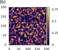
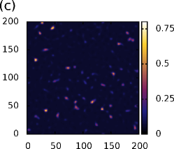
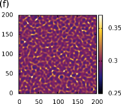
Figure 6: Density profiles displaying evaporation via spinodal decomposition. The top row shows the liquid density profiles and the bottom row shows the nano-particle profiles at times $t/t_{l}=7$ (left), $t/t_{l}=8$ (centre) and $t/t_{l}=9$ (right), where $t_{l}\equiv\frac{\beta}{M_{l}^{nc}}$. The system parameter values are: $k_{B}T=1$, $\epsilon_{l}=1.4$, $\epsilon_{n}=0.6$, $\epsilon_{nl}=0.8$, $M_{l}^{c}=0$, $M_{l}^{nc}=1$, $\alpha=0.5$, $\beta\mu=-4.08$ and $\lambda=0.005$.

The $c=0$ spinodal curve (as calculated in the previous section, Fig. 5) defines the limit of stability, i.e. inside this line the fluid becomes linearly unstable. Thus, the fluid is unstable when $\beta\mu<-3.869$, where $\beta=1/k_{B}T$. The speed of the process increases with decreasing values of $\beta\mu$. For very low values of $\beta\mu$ the evaporation process is so fast that we do not see any pattern formation in the nano-particles - the liquid evaporates too quickly for the nano-particles to diffuse. For the parameters $\epsilon_{l}=1.4$, $\epsilon_{n}=0.6$, $\epsilon_{nl}=0.8$, $\alpha=0.5$, $M_{l}^{c}=0$ and $M_{l}^{nc}=1$ this occurs when $\beta\mu\mathchoice{\mathrel{\vbox{\hbox{$\buildrel\displaystyle<\over{\displaystyle\sim}$}}}}{\mathrel{\vbox{\hbox{$\buildrel\textstyle<\over{\textstyle\sim}$}}}}{\mathrel{\vbox{\hbox{$\buildrel\scriptstyle<\over{\scriptstyle\sim}$}}}}{\mathrel{\vbox{\hbox{$\buildrel\scriptscriptstyle<\over{\scriptscriptstyle\sim}$}}}}-4.2$. Fig. 6 shows the particular case when $\beta\mu=-4.08$. We see that the liquid behaves in a similar manner to that of a single component fluid by spontaneously dewetting everywhere. Now the evaporation is slow enough for the nano-particles to move into areas with a high density of liquid during this evaporative process which creates a fine network structure [as shown in Fig. 6(e) and (f)]. However, this diffusion of the nano-particles is limited as it is still a much slower process than the evaporation of the liquid. We observe that towards the end of the process small heaps of nano-particles are formed, where the density is significantly larger. This effect is enhanced by the attraction between the nano particles ($\epsilon_{n}>0$). Increasing the value of $\mu$, we move from the linearly unstable (spinodal) region into the metastable region of the phase diagram (c.f. Fig. 2). Note however, that the actual values of $\beta\mu$ on the binodal and spinodal now differ from those in Fig. 2 because of the inclusion of nano-particles, c.f. Fig. 4.

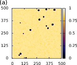
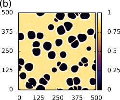
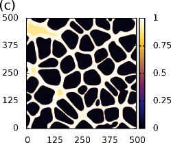
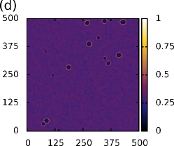
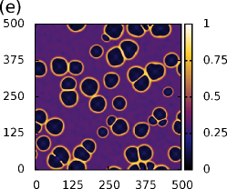
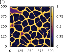
Figure 7: Density profiles displaying nucleation and growth of holes which leads to the development of a network pattern. The top row shows the liquid density profiles and the bottom row shows the nano-particle profiles at times $t/t_{l}=30$ (left), $t/t_{l}=200$ (centre) and $t/t_{l}=800$ (right). The system parameter values are: $k_{B}T=1$, $\epsilon_{l}=1.4$, $\epsilon_{n}=0.6$, $\epsilon_{nl}=0.8$, $M_{l}^{c}=0$, $M_{l}^{nc}=1$, $\alpha=0.5$, $\beta\mu=-3.86$ and $\lambda=0.2$.

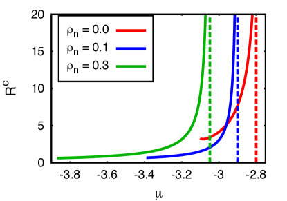
Figure 8: The solid lines display the critical hole radius $R^{c}$ in units of the lattice grid spacing $\sigma$ versus the chemical potential $\mu$ for different nano-particle densities $\rho_{n}$. The lines start at the lowest value of $\mu$ for which the system is linearly stable. The dotted lines show the value of the chemical potential at coexistence $\mu_{\mathrm{coex}}$, which the curves approach asymptotically. Here $k_{B}T=1$, $\epsilon_{l}=1.4$, $\epsilon_{n}=0.6$ and $\epsilon_{nl}=0.8.$

On increasing the chemical potential into the range $-3.869<\beta\mu\mathchoice{\mathrel{\vbox{\hbox{$\buildrel\displaystyle<\over{\displaystyle\sim}$}}}}{\mathrel{\vbox{\hbox{$\buildrel\textstyle<\over{\textstyle\sim}$}}}}{\mathrel{\vbox{\hbox{$\buildrel\scriptstyle<\over{\scriptstyle\sim}$}}}}{\mathrel{\vbox{\hbox{$\buildrel\scriptscriptstyle<\over{\scriptscriptstyle\sim}$}}}}-3.8$, the liquid film becomes metastable but may still evaporate through the nucleation and growth of holes. Fig. 7 shows the case when $\beta\mu=-3.86$. The nucleation is caused by the random fluctuations in the density distributions (the initial density profiles are defined in a similar manner to the previous case: $\rho_{l}(x,t=0)=1-10^{-6}$, $\rho_{n}(x,t=0)=\rho_{n}^{av}+0.4(Y-0.5)$. The amount of noise used and the free energy ‘barrier’ for forming a hole determines the probability of a nucleation event occurring. There is a critical hole radius $R^{c}$ which can be determined from the free-energy of the system. If a hole is smaller than this critical radius then it will shrink and the liquid density will return to its bulk high density value in this region. However, if the size of the hole is larger than this critical value then this hole will begin to grow. We can apply classical nucleation theory to calculate an estimate for the critical hole radius $R^{c}$ by determining the change in free energy $\Delta F$ when a low density (thin film) circular ‘hole’ with a radius of $R$ is inserted into the metastable liquid film. The radius $R$ which corresponds to the maximum in $\Delta F$ is the critical hole radius $R^{c}$. We approximate the change in free energy using the formula:

$$\Delta F=\pi R^{2}\Delta P+2\pi R\gamma,$$ (60)

where $\Delta P$ is the pressure difference between the two phases (the hole and the fluid film). $\gamma$ is the interfacial tension (excess free energy) for creating a straight interface between the two phases at coexistence $\mu=\mu_{\mathrm{coex}}$. It is important to note that the density values at coexistence are different to the density values out of coexistence. The density of the thin film of fluid inside the hole is such that its chemical potential is equal to that of the bulk film of fluid surrounding the hole. The critical hole radius $R^{c}$ is given by the maximum of Eq. (60) - i.e. when $\frac{\partial\Delta F}{\partial R}=0$. Thus, the critical hole radius is $R^{c}=-\frac{\gamma}{\Delta P}$. Fig. 8 shows how $R^{c}$ depends on the chemical potential $\mu$ for different nano-particle densities $\rho_{n}=0$, $0.1$ and $0.3$. This analysis only applies to the metastable region of the phase diagram (c.f. Fig. 2) and therefore the critical hole radius $R^{c}$ curves are bounded on the left by the spinodal curve and on the right by the binodal curve. Note that classical nucleation theory incorrectly predicts a finite value for $R^{c}$ at the spinodal, due to the fact that the theory assumes a sharp interface as one approaches the spinodal. For further discussion on this see e.g.  Ref. [66]. The probability for a hole to be nucleated by random thermal fluctuations is proportional to $e^{-\beta\Delta F}$. The curves in Fig. 8 show that as we approach $\mu_{\mathrm{coex}}$ the size of the critical hole increases. Hence, the probability of nucleation is greater nearer the limit of stability (spinodal curve) and decreases greatly as we approach coexistence (binodal curve). We observe that increasing the density of the nano-particles $\rho_{n}$ shifts the metastable region to lower chemical potential values and increases the range of the metastable region. This is due to the increase in the critical temperature associated with the increase in the nano-particle density $\rho_{n}$, as previously discussed.

In the case shown in Fig. 7, we are near the limit of stability where the critical radius of a hole is very small. This results in many nucleation points where holes are formed and begin to grow. The nano-particles are picked up by these growing holes which creates a rim around each hole with a high density of nano-particles in the rim. The holes in the liquid film continue to grow until their rims meet, creating a random polygonal network pattern of nano-particles. The liquid wets the surface of the nano-particles, which means the liquid remains on the surface in areas with a high density of nano-particles. This is due to the positive interaction energy between the liquid and the nano-particles ($\epsilon_{nl}>0$).

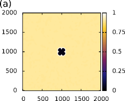
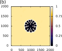
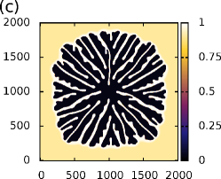
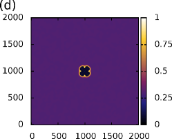
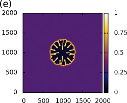
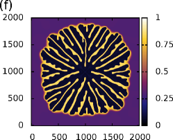
Figure 9: Density profiles displaying the growth of an artificially nucleated point which develops branched structures. The top row shows the liquid density profiles and the bottom row shows the nano-particle profiles at times $t/t_{l}=2000$ (left), $t/t_{l}=10000$ (centre) and $t/t_{l}=30000$ (right). The system parameter values are: $k_{B}T=1$, $\epsilon_{l}=1.4$, $\epsilon_{n}=0.6$, $\epsilon_{nl}=0.8$, $M_{l}^{c}=0$, $M_{l}^{nc}=1$, $\alpha=0.5$, $\beta\mu=-3.8$ and $\lambda=0.1$. Note that instead of using Eq. (59), here the Laplacian term is approximated using: $\nabla^{2}\rho=\frac{1}{6(\Delta x)^{2}}\left(\sum 4\rho^{NN}+\sum\rho^{NNN}-20\rho\right)$.

If we increase the chemical potential further into the metastable range $-3.8\mathchoice{\mathrel{\vbox{\hbox{$\buildrel\displaystyle<\over{\displaystyle\sim}$}}}}{\mathrel{\vbox{\hbox{$\buildrel\textstyle<\over{\textstyle\sim}$}}}}{\mathrel{\vbox{\hbox{$\buildrel\scriptstyle<\over{\scriptstyle\sim}$}}}}{\mathrel{\vbox{\hbox{$\buildrel\scriptscriptstyle<\over{\scriptscriptstyle\sim}$}}}}\beta\mu<\mu_{\mathrm{coex}}$, then the probability of a hole being nucleated becomes much smaller. In an experiment, in this parameter range, all holes that are formed are normally nucleated at defects or impurities of the surface (heterogeneous nucleation). Any interfaces between a high density liquid phase and a low liquid density phase will recede as the liquid evaporates. The velocity of the receding front depends on the value of $\beta\mu$. For small values of $\beta\mu$ we have a fast front, but the speed of the front reduces as $\mu$ approaches $\mu_{\mathrm{coex}}$. If we choose $\mu=\mu_{\mathrm{coex}}$ then any straight front remains stationary. On a completely structureless substrate, one would usually expect such an interface to recede homogeneously; this is certainly the case for the pure liquid, when $\rho_{n}=0$. However, in our system when $\rho_{n}>0$ we see the formation of fingers as the front recedes, due to the presence of the nano-particles. Fig. 9 shows a case when $\beta\mu=-3.8$. The initial density profiles in this situation differ slightly from the previous cases. Here we create an artificial nucleation point by setting the density of the liquid and the nano-particles to $\rho_{l}=\rho_{n}=10^{-6}$ in a central $2\sigma\times 2\sigma$ region. Without this seed nucleus the initial noise on the density profiles slowly decays and the densities of the two species return to their (metastable) equilibrium values. The liquid surrounding this nucleation point slowly recedes creating a circular dewetting front. As the front recedes, it begins to collect the nano-particles, as was also observed for the case in Fig. 7. However, here the growing hole does not meet any other holes and there is time for an instability to develop at the front which causes the liquid to evaporate faster in some regions and slower in others creating a ‘wavy’ front, as seen in Fig. 9(a) and Fig. 9(d). The ‘bumps’ at the front then appear to stop moving while the rest of the front continues to recede. As the front recedes and the hole circumference increases, more fingers develop, leaving a branched ‘fingered’ nano-particle structure behind – Figs. 9(e) and (f). The time scale for this dewetting process is rather long and so we also observe some long-time coarsening effects on the finger structures.

Recall that one of the goals of our work is to develop an understanding of how the different self-organised structures of nano-particles observed in the experiments [22, 25, 26, 23] are formed. Distinct observed structures are a) network structures and b) branched structures. Results from our model have shown how two different types of network structures can develop: i) a fine network structure created by a spinodal evaporation process (Fig. 6) in which the nano-particle density varies over a fairly small range $0.27\mathchoice{\mathrel{\vbox{\hbox{$\buildrel\displaystyle<\over{\displaystyle\sim}$}}}}{\mathrel{\vbox{\hbox{$\buildrel\textstyle<\over{\textstyle\sim}$}}}}{\mathrel{\vbox{\hbox{$\buildrel\scriptstyle<\over{\scriptstyle\sim}$}}}}{\mathrel{\vbox{\hbox{$\buildrel\scriptscriptstyle<\over{\scriptscriptstyle\sim}$}}}}\rho_{n}\mathchoice{\mathrel{\vbox{\hbox{$\buildrel\displaystyle<\over{\displaystyle\sim}$}}}}{\mathrel{\vbox{\hbox{$\buildrel\textstyle<\over{\textstyle\sim}$}}}}{\mathrel{\vbox{\hbox{$\buildrel\scriptstyle<\over{\scriptstyle\sim}$}}}}{\mathrel{\vbox{\hbox{$\buildrel\scriptscriptstyle<\over{\scriptscriptstyle\sim}$}}}}0.45$, ii) a large well defined network structure created by the nucleation and growth of holes in the liquid (Fig. 7), in which the nano-particle density varies over a large range $0.05\mathchoice{\mathrel{\vbox{\hbox{$\buildrel\displaystyle<\over{\displaystyle\sim}$}}}}{\mathrel{\vbox{\hbox{$\buildrel\textstyle<\over{\textstyle\sim}$}}}}{\mathrel{\vbox{\hbox{$\buildrel\scriptstyle<\over{\scriptstyle\sim}$}}}}{\mathrel{\vbox{\hbox{$\buildrel\scriptscriptstyle<\over{\scriptscriptstyle\sim}$}}}}\rho_{n}\mathchoice{\mathrel{\vbox{\hbox{$\buildrel\displaystyle<\over{\displaystyle\sim}$}}}}{\mathrel{\vbox{\hbox{$\buildrel\textstyle<\over{\textstyle\sim}$}}}}{\mathrel{\vbox{\hbox{$\buildrel\scriptstyle<\over{\scriptstyle\sim}$}}}}{\mathrel{\vbox{\hbox{$\buildrel\scriptscriptstyle<\over{\scriptscriptstyle\sim}$}}}}0.9$. Our model also shows how instabilities at the evaporative dewetting front can create branched structures for certain parameter values (Fig. 9). Note that there is also evidence of early stages of the fingering instability in the nucleation case shown in Fig. 7. There one can observe that small bumps begin to develop in the edges of some of the larger holes. We now consider the formation of the branched structures in more detail. In particular, we investigate the dependence of these ‘fingered’ structures on the parameters of the model.

5.3 Influence of mobilities on the fingering

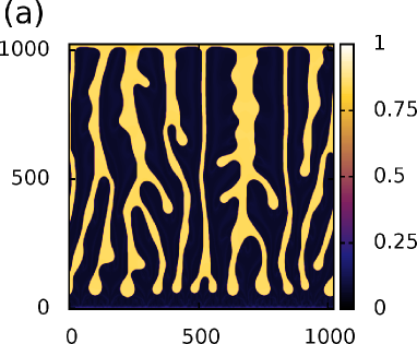
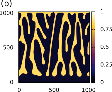
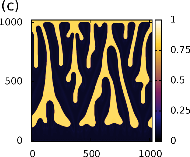
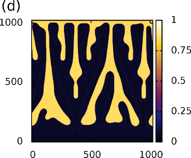
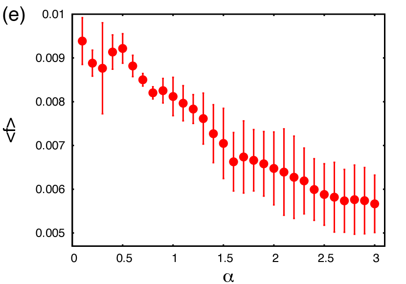
Figure 10: Nano-particle density profiles for calculations with (a) $\alpha=0.1$, (b) $\alpha=1$, (c) $\alpha=2$ and (d) $\alpha=3$. In (e) we display a plot showing the dependence of the number of fingers on the parameter value $\alpha$. The parameter values are: $k_{B}T=1$, $\epsilon_{l}=1.4$, $\epsilon_{n}=0.6$, $\epsilon_{nl}=0.8$, $M_{l}^{c}=0$, $M_{l}^{nc}=1$, $\beta\mu=-3.8$, $\Delta x=1$ and $\lambda=0.1$.

To make a detailed investigation of the branched finger structures it is important to maximise the distance a front can recede. This allows us to obtain better statistics which is important due to the fact that solving the DDFT in the fingering regime on a large grid can be time consuming. To achieve this objective we create a straight dewetting front along the bottom edge of the system (i.e. we set the two density values to $\rho_{l}=\rho_{n}=10^{-6}$ for the first five horizontal lines). We also set no-flux boundary conditions at the top and the bottom, to prevent a dewetting front forming at the top. The periodic boundary conditions on the left and the right side of the system domain remain. This set-up also allows for easier analysis of the branched structures since we begin with an initially straight front. We define a measure for the average number of fingers $\langle f\rangle$ to be the average number of branched structures per unit length in the final density profile, after the dewetting front has reached the top of the system. To calculate this quantity we implemented an algorithm which counts the number of transitions between a high density of nano-particles and a low density of nano-particles on each horizontal line of the system. We then determine the number of fingers on a given horizontal line by dividing this value by two. We set a minimum and maximum line for a given set of final density profiles and calculate the average number of fingers between these two lines. This value is then divided by the size of the system to give a value that is independent of the system size. We have investigated how this measure is affected by the different parameters of the system.

We begin by discussing the effect that varying the parameter $\alpha$ has on $\langle f\rangle$ (recall that $\alpha$ determines the mobility of the nano-particles in the liquid film). We use the same parameter values as above, with $\beta\mu=-3.8$ and $\alpha$ varying between $0.1$ and $3$. Fig. 10 shows final nano-particle density profiles for several values of $\alpha$ and also a plot of $\langle f\rangle$ versus $\alpha$, which is calculated from the average of five runs. We see that the value of $\alpha$ has a significant influence on the average finger number. Increasing the mobility of the nano-particles results in fewer fingers being developed, which is in (qualitative) agreement with the experiments [23] and the KMC model results [29]. The mobility of the nano-particles directly influences the speed of the receding front, so evaporation is much slower when $\alpha$ is small. When $\alpha$ is very small ($\alpha\mathchoice{\mathrel{\vbox{\hbox{$\buildrel\displaystyle<\over{\displaystyle\sim}$}}}}{\mathrel{\vbox{\hbox{$\buildrel\textstyle<\over{\textstyle\sim}$}}}}{\mathrel{\vbox{\hbox{$\buildrel\scriptstyle<\over{\scriptstyle\sim}$}}}}{\mathrel{\vbox{\hbox{$\buildrel\scriptscriptstyle<\over{\scriptscriptstyle\sim}$}}}}0.002$) we find that the two density fields become practically decoupled, with the liquid evaporating at high speed leaving the nano-particles behind as a homogeneous film of the initial density $\rho_{n}^{av}$.

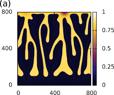
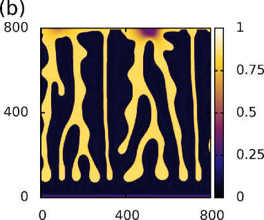
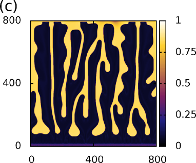
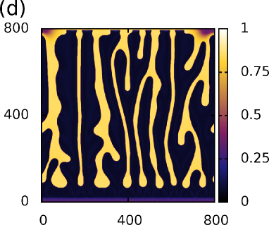
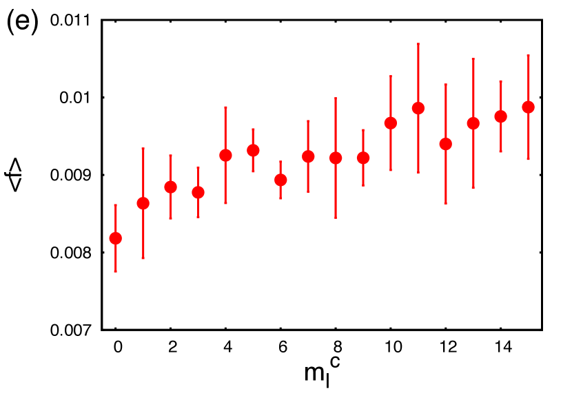
Figure 11: Nano-particle density profiles for (a) $M_{l}^{c}=0$, (b) $M_{l}^{c}=5$, (c) $M_{l}^{c}=10$ and (d) $M_{l}^{c}=15$. In (e) we display a plot showing how the number of fingers $\langle f\rangle$ depends on the value of $M_{l}^{c}$. The parameter values are: $k_{B}T=1$, $\epsilon_{l}=1.4$, $\epsilon_{n}=0.6$, $\epsilon_{nl}=0.8$, $M_{l}^{nc}=1$, $\alpha=1$, $\beta\mu=-3.8$ and $\lambda=0.1$.

The effect of liquid diffusion over the surface has also been investigated by varying the liquid conserved mobility $M_{l}^{c}$. Using the same parameter values as above, and setting $\alpha=1$, we display in Fig. 11 final nano-particle density profiles for varying $M_{l}^{c}$ from 0 to 15 and also the average finger number $\langle f\rangle$ versus $M_{l}^{c}$ averaged over five runs. We see that the diffusive mobility of the liquid $M_{l}^{c}$ does affect the average number of fingers but to a much smaller extent than the mobility of the nano-particles. The average finger number generally increases as $M_{l}^{c}$ is increased.

5.4 Influence of liquid-particle demixing on the fingering

We now discuss the effect of possible liquid-particle phase separation on the front instability. Such a phase separation may occur near the front even for nano-particle concentrations inside the liquid film that are far smaller than the binodal value for liquid-particle phase separation. This occurs because as a dewetting front recedes it collects nano-particles (as previously discussed) and therefore increases the value of $\rho_{n}$ near the front. For certain parameter values we find that if $\rho_{n}$ increases above a certain threshold value, then liquid-particle phase separation occurs in the front region. The liquid separates into two liquid phases, a mobile one poor in colloids and a less mobile one rich in colloids. To investigate the resulting effects we set the interaction energies to $\epsilon_{l}=1.7$, $\epsilon_{nl}=1$ and vary $\epsilon_{n}$ from $0$ to $1.2$. Eq. (58) indicates that we should observe liquid-particle phase separation for $\epsilon_{n}>0.3$. We set the average nano-particle density to be low, $\rho_{n}^{av}=0.1$, so that there is no liquid-particle phase separation in the bulk of the fluid film. For the value of the chemical potential that we use $\mu=-4$, the fluid is linearly stable for all values of $\epsilon_{n}$ and leads to a relatively fast dewetting front.

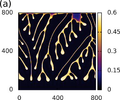
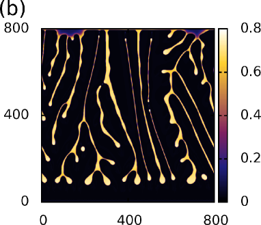
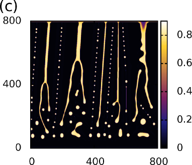
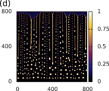
Figure 12: Nano-particle density profiles for (a) $\epsilon_{n}=0.3$, (b) $\epsilon_{n}=0.6$, (c) $\epsilon_{n}=0.8$ and (d) $\epsilon_{n}=1.1$. In (e) we display a plot showing how the mean number of fingers $\langle f\rangle$ depends on the parameter $\epsilon_{n}$. When $\epsilon_{n}>0.6$ we begin to observe droplets being deposited along with the branched structures (as shown in (c)). The parameter values for these calculations are: $k_{B}T=1$, $\epsilon_{l}=1.7$, $\epsilon_{nl}=1.0$, $M_{l}^{c}=0$, $M_{l}^{nc}=1$, $\alpha=0.5$, $\mu=-4$, $\rho_{n}^{av}=0.1$ and $\lambda=0.025$.

In Fig. 12(a)-(d) we display typical final nano-particle density profiles for various $\epsilon_{n}$ and the average finger number $\langle f\rangle$ versus $\epsilon_{n}$, averaged over five runs. As $\epsilon_{n}$ is increased from $\epsilon_{n}=0$, we initially see a linear increase in the average number of fingers $\langle f\rangle$. This reaches a peak at $\epsilon_{n}\approx 0.6$, after which we begin to see the development of droplets. When $0.6\mathchoice{\mathrel{\vbox{\hbox{$\buildrel\displaystyle<\over{\displaystyle\sim}$}}}}{\mathrel{\vbox{\hbox{$\buildrel\textstyle<\over{\textstyle\sim}$}}}}{\mathrel{\vbox{\hbox{$\buildrel\scriptstyle<\over{\scriptstyle\sim}$}}}}{\mathrel{\vbox{\hbox{$\buildrel\scriptscriptstyle<\over{\scriptscriptstyle\sim}$}}}}\epsilon_{n}\mathchoice{\mathrel{\vbox{\hbox{$\buildrel\displaystyle<\over{\displaystyle\sim}$}}}}{\mathrel{\vbox{\hbox{$\buildrel\textstyle<\over{\textstyle\sim}$}}}}{\mathrel{\vbox{\hbox{$\buildrel\scriptstyle<\over{\scriptstyle\sim}$}}}}{\mathrel{\vbox{\hbox{$\buildrel\scriptscriptstyle<\over{\scriptscriptstyle\sim}$}}}}0.9$ we observe separation between regions of high density of nano-particles and low density of nano-particles occurring locally at the dewetting front. The areas with a lower density of nano-particles form very thin fingers which quickly rupture into a series of droplets, whereas the areas with a higher density form thicker fingers which are much more stable as shown in Fig. 12(c). The sections of the front with a lower density of nano-particles recede faster than the rest of the front. This results in a ‘doublon’ pattern which has been observed in many different systems, e.g.  in the thin film directional solidification of a nonfaceted cubic crystal [67]. As we increase $\epsilon_{n}$ further, for $\epsilon_{n}>1$ we observe that the dynamics at the front remains similar, however, now all the finger structures are very thin and therefore quickly break up into droplets. One also notices that the tendency to form side branches decreases with increasing $\epsilon_{n}$ whereas the orientation of the branches becomes increasingly perpendicular to the receding front. We also observe an increase in the density of the nano-particles within the fingers/droplets as $\epsilon_{n}$ is increased. This is due to the increased attraction between the nano-particles. These results agree qualitatively with the KMC model [29]. The KMC results also show an initial increase in the number of fingers followed by a transition from fingers to droplets as the interaction energy between the nano-particles $\epsilon_{n}$ is increased. Fig. 17 of Ref. [29] displays a plot of $\langle f\rangle$ versus $\epsilon_{n}$ which shows a similar trend as the DDFT results displayed in Fig. 12(e). However, as it is a discrete stochastic model, the details of the transition in the way the branching occurs are less discernible than in the present DDFT model.

6 Concluding remarks

We have presented a DDFT based model for the evaporative dewetting of an ultrathin film of a colloidal suspension. We have derived an expression for the free energy of the system using a mean-field approximation for a coarse-grained Hamiltonian model (1) for the system. We have also derived dynamical equations which describe the diffusive dynamics of the solvent and of the colloids as well as the evaporation of the solvent. We have considered the equilibrium phase behaviour of the pure solvent and of the two-component fluid and identified parameter ranges where unstable, metastable and stable phases exist. We then solved the coupled dynamical equations numerically to investigate the different dynamical pathways of the phase transition and the resulting self-organised patterns of the nano-particles.

The model successfully describes the various self-organised structures found in experiments [23] and is in qualitative agreement with the discrete stochastic KMC model [29]. Our numerical results show how nano-particle network structures can form either from a spinodal processes (Fig. 6) or through the nucleation and growth of holes (Fig. 7). We have also observed how branched structures develop from a fingering instability of the receding dewetting front (Fig. 9).

The transverse front instability results from a build-up of the nanoparticles close to the front as the solvent evaporates, when diffusion is too slow to disperse them. This slows down the front and renders it unstable. As a result, density fluctuations along the front grow into an evolving fingering pattern. This transverse front instability can be considered to be a self-optimisation process which maintains the mean front velocity constant [29] (see also the discussion of this in the context of a similar front instability occurring in the dewetting of non-volatile polymer films [68]). One may also say that the constant average front velocity is maintained by depositing some of the nano-particles onto the dry substrate creating the branched structures. Experimental observations show that the branched structures found in the ultra-thin film behind the mesoscopic dewetting front are initiated from random nucleation sites. The holes which are nucleated then grow, initially creating circular dewetting fronts. We subsequently observe that the fingering instabilities and the development of branched structures form on the circular interfaces. Fig. 9 shows how these circular branched patterns develop from a single nucleation point; our numerical results bare a striking resemblance to the experimental AFM images of this phenomena [23].

We have studied the branched structures in greater detail using a planar geometry, i.e., by creating initially straight dewetting fronts. We have considered how the different mobilities affect the fingering. The nano-particle mobility in liquid films has a significant effect on the average number of fingers in the branched structure (Fig. 10). The finger number decreases rapidly with increasing mobility in agreement with earlier KMC results [29]. This behaviour can be attributed to the lower-mobility of the nano-particles that hinders re-distribution by diffusion and also reduces the speed of the dewetting front. For the system to attain a higher front speed it must deposit nano-particles onto the surface at a greater rate. Therefore, if the mobility of the nano-particles is low this leads to the creation of more fingers because in this case the average distance a nano-particle has to travel to reach a finger is smaller. Increasing the mobility for the conserved diffusive dynamics of the liquid has the opposite effect on the average number of fingers (Fig. 11). The complex relationship between the diffusion of the liquid and the average finger number is not yet fully understood. Our hypothesis is that increasing the mobility of the liquid results in an effective increase in the speed of the dewetting dynamics of the liquid for fixed nano-particle mobility. Thus, the mobility of the nano-particles becomes lower in comparison. The increased finger number then results from the increased mobility contrast, in agreement with the general instability mechanism laid out above.

The basic front instability as described above is a purely dynamic effect and does not depend on particle-liquid and particle-particle attractive interactions that favour demixing of the liquid and the nanoparticles. However, beside this regime (that we call the ‘transport regime’) we have investigated how interactions that favour demixing influence the instability (Fig. 12). In general, when increasing the interaction energy between the nano-particles one increases the tendency towards liquid-particle demixing. However, this has no practical effect as long as the nano-particle concentration is low, so that it is outside of the two-phase region. This is normally the case for our initial densities. However, in the course of the evaporative dewetting the density increases close to the receding front. Increasing the interaction energy between the nano-particles causes demixing to occur close to the front (but not in the bulk film). The demixing makes the fingering instability stronger (we call this the ‘demixing regime’). At first, one finds a linear increase in the average finger number with increasing interaction energy. At higher values of $\epsilon_{n}$, when the localised phase separation sets in, the fingers become straight with less side branches, before finally lines of drops are emitted directly at the front. In this regime, the mean number of fingers is determined by the dynamics and the energetics of the system.

The results we have obtained with our DDFT model confirm that jamming of discrete particles (as already discussed in Ref. [37]) is not a necessary factor for the fingering instability to occur. Our model is a continuum model with a diffusion constant that is independent of the nanoparticle concentration. The present two-dimensional DDFT model has several advantages over the two-dimensional KMC model [28, 29]: In particular, the early instability stages are more easy to discern without the background noise of the KMC. Furthermore, the underlying free energy may be employed to analyse the equilibrium phase behaviour in detail, in a similar manner to Ref. [53]. Many standard tools for the analysis of partial differential equations can be applied to the coupled evolution equations, such as, e.g., the linear stability analysis of the homogeneous films. In the future, one may perform a linear stability analysis for the receding straight front and also investigate steady state solutions as has been done for evaporating films of pure liquids [49]. There are many details that would merit further investigations such as, for example, the doublon structure mentioned in Section 5.4 and its relation to such structures formed in directional solidification [69].

The present DDFT model does not include the effect of surface forces, i.e., wettability effects (substrate-film interactions). Therefore, a non-volatile liquid film would not dewet the substrate. This implies that an important avenue for future improvement is to incorporate wettability effects into the model. This could be done by making a mean-field approximation to derive an expression for the free energy for a fully three-dimensional KMC model [70, 71] (after incorporating substrate-particle and substrate-liquid interactions). The resulting three-dimensional DDFT could then either be used directly or be averaged perpendicularly to the substrate employing e.g., a long-wave approximation. Another possible option consists of combining a mesoscopic hydrodynamic approach, e.g., a thin film evolution equation (see [31, 72, 49]) with elements of DDFT. For a brief discussion of a similar approach see Ref. [73].

As a final remark, we recall that in the present work we have only considered dewetting from homogeneous substrates. However, it is straightforward to include surface heterogeneities in our model via the external potentials $\phi_{i}({\bf r})$ in Eq. (8). As future work, it would be interesting to study the influence of surface patterning on the finger formation displayed by the present system.

References

References

- [1] A. Giacometti, A. Maritan, and J. R. Banavar, Phys. Rev. Lett. 75, 577 (1995).
- [2] M. Mimura, H. Sakaguchi, and M. Matsushita, Physica A 282, 283 (2000).
- [3] A. Yochelis, Y. Tintut, L. L. Demer, and A. Garfinkel, New J. Phys. 10, 055002 (2008).
- [4] Y. A. Vlasov, X-Z. Bo, J. C. Sturm, and D. J. Norris, Nature 414, 289 (2001).
- [5] V. S. Mitlin, J. Colloid Interface Sci. 156, 491 (1993).
- [6] G. Reiter, Phys. Rev. Lett. 68, 75 (1992).
- [7] R. Xie et al., Phys. Rev. Lett. 81, 1251 (1998).
- [8] R. Seemann, S. Herminghaus, and K. Jacobs, Phys. Rev. Lett. 86, 5534 (2001).
- [9] U. Thiele, M. G. Velarde, and K. Neuffer, Phys. Rev. Lett. 87, 016104 (2001).
- [10] U. Thiele, Eur. Phys. J. E 12, 409 (2003).
- [11] J. Becker et al., Nat. Mater. 2, 59 (2003).
- [12] P. Beltrame and U. Thiele, SIAM J. Appl. Dyn. Syst. 9, 484 (2010).
- [13] C. Redon, F. Brochard-Wyart, and F. Rondelez, Phys. Rev. Lett. 66, 715 (1991).
- [14] A. Sharma and G. Reiter, J Colloid Interface Sci. 178, 383 (1996).
- [15] A. Sharma and R. Khanna, Phys. Rev. Lett. 81, 3463 (1998).
- [16] M. Bestehorn and K. Neuffer, Phys. Rev. Lett. 87, 046101 (2001).
- [17] U. Thiele, M. Mertig, and W. Pompe, Phys. Rev. Lett. 80, 2869 (1998).
- [18] X. Gu, D. Raghavan, J. F. Douglas, and A. Karim, J. Polym. Sci. Pt. B-Polym. Phys. 40, 2825 (2002).
- [19] L. Xu, T. F. Shi, P. K. Dutta, and L. An, J. Chem. Phys. 127, 144704 (2007).
- [20] M. Maillard, L. Motte, A. T. Ngo, and M. P. Pileni, J. Phys. Chem. B 104, 11871 (2000).
- [21] G. L. Ge and L. Brus, J. Phys. Chem. B 104, 9573 (2000).
- [22] P. Moriarty, M. D. R. Taylor, and M. Brust, Phys. Rev. Lett. 89, 248303 (2002).
- [23] E. Pauliac-Vaujour et al., Phys. Rev. Lett. 100, 176102 (2008).
- [24] A. Stannard, J. Phys.: Condens. Matter 23, 083001 (2011).
- [25] C. P. Martin, M. O. Blunt, and P. Moriarty, Nano Lett. 4, 2389 (2004).
- [26] C. P. Martin et al., Phys. Rev. Lett. 99, 116103 (2007).
- [27] E. Pauliac-Vaujour and P. Moriarty, J. Phys. Chem. C 111, 16255 (2007).
- [28] E. Rabani, D. R. Reichman, P. L. Geissler, and L. E. Brus, Nature 426, 271 (2003).
- [29] I. Vancea et al., Phys. Rev. E 78, 041601 (2008).
- [30] A. Stannard et al., J. Chem. Phys. C 112, 15195 (2008).
- [31] A. Oron, S. H. Davis, and S. G. Bankoff, Rev. Mod. Phys. 69, 931 (1997).
- [32] L. Frastia, A.J. Archer, and U. Thiele, Phys. Rev. Lett. 106, 077801 (2011).
- [33] H. Yabu and M. Shimomura, Adv. Funct. Mater. 15, 575 (2005).
- [34] J. Xu et al., Phys. Rev. Lett. 96, 066104 (2006).
- [35] J. Xu, J. F. Xia, and Z. Q. Lin, Angew. Chem.-Int. Edit. 46, 1860 (2007).
- [36] H. Bodiguel, F. Doumenc, and B. Guerrier, Langmuir 26, 10758 (2010).
- [37] U. Thiele et al., J. Phys.: Condens. Matter 21, 264016 (2009).
- [38] A. J. Archer, M. J. Robbins, and U. Thiele, Phys. Rev. E 81, 021602 (2010).
- [39] U. M. B. Marconi and P Tarazona, J. Chem. Phys. 110, 8032 (1999).
- [40] U. M. B. Marconi and P Tarazona, J. Phys.: Condens. Matter 12, A413 (2000).
- [41] A. J. Archer and R. Evans, J. Chem. Phys. 121, 4246 (2004).
- [42] A. J. Archer and M. Rauscher, J. Phys. A. 37, 9325 (2004).
- [43] J. F. Gouyet, M Plapp, W Dieterich, and P Maass, Adv. Phys. 52, 523 (2003).
- [44] P. M. Chaikin and T. C. Lubensky, Principles of Condensed Matter Physics (Cambridge University Press, Cambridge, 2000).
- [45] J. P. Hansen and I. R. McDonald, Theory of simple liquids (Academic Press, London, 2006).
- [46] R. Evans, Adv. Phys. 28, 143 (1979).
- [47] R. Evans, in Fundamentals of inhomogeneous fluids, edited by D. Henderson (Dekker, New York, 1992), Chap. 3.
- [48] A. V. Lyushnin, A. A. Golovin, and L. M. Pismen, Phys. Rev. E 65, 021602 (2002).
- [49] U. Thiele, J. Phys.: Cond. Mat. 22, 084019 (2010).
- [50] J. W. Cahn and J. E. Hilliard, J. Chem. Phys. 28, 258 (1958).
- [51] J. W. Cahn, J. Chem. Phys. 42, 93 (1965).
- [52] J. S. Langer, in Solids far from Equilibrium, edited by C. Godreche (Cambridge University Press, Cambridge, 1992), Chap. 3, pp. 297–363.
- [53] D. Woywod and Schoen M., Phys. Rev. E 73, 011201 (2006).
- [54] A. Pototsky, M. Bestehorn, D. Merkt, and U. Thiele, J. Chem. Phys. 122, 224711 (2005).
- [55] A. J. Archer and R. Evans, Phys. Rev. E. 64, 041501 (2001).
- [56] J. S. Rowlinson and F. L. Swinton, Liquids and Liquid Mixtures, 3rd ed. (Butterworth Scientific, London, 1982).
- [57] L. Leibler, Macromolecules 13, 1602 (1980).
- [58] Y. Nishiura and I. Ohnishi, Phys. D 84, 31 (1995).
- [59] A. J. Archer and N. B. Wilding, Phys. Rev. E 76, 031501 (2007).
- [60] R. P. Sear et al., Phys. Rev. E 59, R6255 (1999).
- [61] A. I. Campbell, V. J. Anderson, J. S. van Duijneveldt, and P. Bartlett, Phys. Rev. Lett. 94, 208301 (2005).
- [62] A. Stradner et al., Nature 432, 492 (2004).
- [63] H. Sedgwick, S. U. Egelhaaf, and W. C. K Poon, J. Phys.: Condens. Matter 16, S4913 (2004).
- [64] G. Brown, P. A. Rikvold, M. Sutton, and M. Grant, Phys. Rev. E 56, 6601 (1997).
- [65] S. Fomel and J. F. Claerbout, Stanford Exploration Project 95, 43 (1997).
- [66] D. W. Oxtoby and R. Evans, J. Chem. Phys. 89, 7521 (1988).
- [67] S. Akamatsu, G. Faivre, and T. Ihle, Phys. Rev. E. 51, 4751 (1995).
- [68] G. Reiter and A. Sharma, Phys. Rev. Lett. 87, 166103 (2001).
- [69] B. Utter and E. Bodenschatz, Phys. Rev. E 72, 011601 (2005).
- [70] C. G. Sztrum, O. Hod, and E. Rabani, J. Phys. Chem. B 109, 6741 (2005).
- [71] G. Yosef and E. Rabani, J. Phys. Chem. B 110, 20965 (2006).
- [72] D. Bonn et al., Rev. Mod. Phys. 81, 739 (2009).
- [73] U. Thiele, Eur. Phys. J. Special Topics D& D (2011), at press.