Resonant invisibility with finite range interacting fermions

Abstract

We study the eigenstates of two opposite spin fermions on a one-dimensional lattice with finite range interaction. The eigenstates are projected onto the set of Fock eigenstates of the noninteracting case. We find antiresonances for symmetric eigenstates, which eliminate the interaction between two symmetric Fock states when satisfying a corresponding selection rule.

Introduction. Up to now a lot of interest in experiments on cold atoms has been focused on matter wave properties of the condensates which are described by the Hartree-Fock-Bogoliubov mean field model for weakly interacting quantum gases Nature416 ; Dalfogo71 ; Legett73 ; Pitaevskii2003 ; Pethick2001 . At the same time, the use of collision processes turns out to be a promising approach to implement quantum gate operations Mendel2003 . A standard method for the description of such systems is to map them to Hubbard like lattice models where atomic physics provides a whole toolbox to engineer various types of Hamiltonians for 1D, 2D, and 3D Bose and Fermi systems.

The interplay of interactions and discreteness leads to a set of interesting phenomena, including bound states, see e.g. Fleurov ; Scott1 ; Pinto ; Pinto2007 ; Pinto2008 and EilbeckPhysicaD78 ; Dorignac2004 ; Pouthier2003PRE . In recent papers NguenangPRB75 ; jpnflach09PhysRevA80 we have studied properties of such bound states (also frequently coined quantum breathers) in various one dimensional Hubbard like models by considering two bosons or two fermions (with opposite spins) on lattices. The fermionic case adds to the complexity with the spin as an additional degree of freedom. Consequently two fermions can form up to three different bound states, while two bosons form only one. In all these cases the interaction was assumed to be local, i.e. both particles interact only when occupying the same lattice site. In the present paper we consider fermionic particles with a finite range of interaction, as a more realistic description of experimental situations, which may be directly applicable in quantum computing, where the controlled interaction can be used to create entanglement with high fidelity. We analyze two particle eigenfunctions and identify resonance conditions for which two particles do not scatter despite the presence of a nonzero interaction.

Model and spectrum. We consider one-dimensional periodic lattice with $f$ sites described by an extended fermionic Bose-Hubbard (EFBH) model. The Hamiltonian is given by

$$\hat{H}=\hat{H}_{0}+\hat{H}_{U}+\hat{H}_{V},$$ (1)

$$\hat{H}_{0}=-\sum_{j,\sigma}\hat{a}_{j,\sigma}^{+}(\hat{a}_{j-1,\sigma}+\hat{a}_{j+1,\sigma}),$$ (2)

$$\hat{H}_{U}=-U\sum_{j}\hat{n}_{j,\uparrow}\hat{n}_{j,\downarrow},{\ }{\ }{\ }{\ }{\ }\hat{n}_{j,\sigma}=\hat{a}_{j,\sigma}^{+}\hat{a}_{j,\sigma},$$ (3)

$$\hat{H}_{V}=-V\sum_{j}\hat{n}_{j}\hat{n}_{j+1},{\ }{\ }{\ }\hat{n}_{j}=\hat{n}_{j,\uparrow}+\hat{n}_{j,\downarrow}.$$ (4)

Here $\hat{H}_{0}$ describes the nearest-neighbor hopping, $\sigma=\uparrow$,$\downarrow$ denotes the spin, $\hat{H}_{U}$ and $\hat{H}_{V}$ describe the onsite and intersite (between adjacent sites) interaction between the particles with strengths $U$, and $V$, respectively; $a_{j,{\sigma}}^{+}$ and $a_{j,{\sigma}}$ are the fermionic creation and annihilation operators satisfying the anticommutation relations: $[\hat{a}_{j,{\sigma}},\hat{a}_{l,{\sigma}^{\prime}}^{+}]=\delta_{j,l}\delta_{\sigma,\sigma^{\prime}}$, and $[\hat{a}_{j,{\sigma}},\hat{a}_{l,\sigma^{\prime}}]=[\hat{a}_{j,{\sigma}}^{+},\hat{a}_{l,\sigma^{\prime}}^{+}]=0$. The sign of $U$ and $V$ is not specified. The Hamiltonian (1) commutes with the number operator $\hat{N}=\sum_{j}\hat{n}_{j}$ whose eigenvalues are $n=n_{\uparrow}+n_{\downarrow}$, which is the total number of fermions in the lattice. In this work we focus on the simplest nontrivial case of $n=2$, with $n_{\uparrow}=1$ and $n_{\downarrow}=1$.

To describe quantum states, we use a number state basis $|\Phi_{n}\rangle=|n_{1};n_{2}\cdots n_{f}\rangle$ EilbeckPhysicaD78 , where $n_{i}=n_{i,{\uparrow}}+n_{i,{\downarrow}}$ represents the number of fermions at the i-th site of the lattice. The fermionic two particle states are generated from the vacuum $|O\rangle$ by successively creating a particle with spin down and spin up.

The Hamiltonian (1) commutes with the translational operator $\hat{T}$, which shifts all lattice indices by one. Its eigenvalues are $\tau=exp(ik)$ with the Bloch wave number $k=\frac{2\pi\nu}{f}$, and $\nu=0,1,2,\cdots,f-1$ .

Single-fermion states. In this simplest case, only one fermion is in the lattice (either with spin up or down) ($n=1$), and the state is represented by $|j\rangle=\hat{a}_{j,\sigma}^{+}|O\rangle$. The interaction terms ($\hat{H}_{U}$ and $\hat{H}_{V}$ ) have no contribution for a single particle. Thus the eigenstates of the Hamiltonian (1) are the eigenstates of $\hat{H}_{0}$ which are given by:

$$|\Psi_{1}\rangle=\frac{1}{\sqrt{f}}\sum_{s=1}^{f}\Big{(}\frac{\hat{T}}{\tau}\Big{)}^{s-1}|1\rangle\;.$$ (5)

The corresponding eigenenergies are

$$\varepsilon_{k}=-2\cos(k)\;.$$ (6)

Two fermions. For the case of two opposite spin fermions ($n=2$ with $n_{\uparrow}=1$ and $n_{\downarrow}=1$), each eigenstate is formed as a linear combination of number states with fixed $n$.

$$|\Psi_{n}\rangle=\sum_{j}c_{j}|\Phi_{n}^{j}\rangle\;.$$ (7)

For two particles, this involves $N_{s}=f^{2}$ basis states, $|\Phi_{2}^{j}\rangle$, which is the number of ways one can distribute two fermions with opposite spins over the $f$ sites with possible double occupancy. Then we define the basis state with a given value of the wave number $k$ as in Ref. jpnflach09PhysRevA80 and a complete wave function is:

$$|\Psi_{2}^{k}\rangle=c_{1}|\Phi_{1}\rangle+\sum_{j=2}^{(f+1)/2}c_{j,+}|\Phi_{j,+}\rangle+\sum_{j=2}^{(f+1)/2}c_{j,-}|\Phi_{j},-\rangle\;.$$ (8)

Any vector in the corresponding Hilbert space is spanned by the numbers $|c_{1},c_{2,+},c_{2,-},c_{3,+},c_{3,-}\cdots\rangle$ and the vectors $|\Phi_{1}\rangle$, $|\Phi_{j,+}\rangle$ and $|\Phi_{j,-}\rangle$ in two fermion case are defined as follows:

$$|\Phi_{1}\rangle=\frac{1}{\sqrt{f}}\sum_{s=1}^{f}\Big{(}\frac{\hat{T}}{\tau}\Big{)}^{s-1}\hat{a}_{1,\uparrow}^{+}\hat{a}_{1,\downarrow}^{+}|O\rangle;$$

$$|\Phi_{j,+}\rangle=\frac{1}{\sqrt{f}}\sum_{s=1}^{f}\Big{(}\frac{\hat{T}}{\tau}\Big{)}^{s-1}\hat{a}_{j,\uparrow}^{+}\hat{a}_{1,\downarrow}^{+}|O\rangle;$$ (9)

$$|\Phi_{j,-}\rangle=\frac{1}{\sqrt{f}}\sum_{s=1}^{f}\Big{(}\frac{\hat{T}}{\tau}\Big{)}^{s-1}\hat{a}_{1,\uparrow}^{+}\hat{a}_{j,\downarrow}^{+}|O\rangle;$$

We diagonalize the Hamiltonian (1) in the framework of the basis defined in (8) and derive the eigenenergies for each given Bloch wave number $k$ from $\hat{H}|\Psi_{2}^{k}\rangle=E|\Psi_{2}^{k}\rangle$. This leads to an $f\times f$ matrix whose elements $H_{i,j}$ ($i,j=2,\ldots,(f+1)/2$) are derived from

$$H_{i,1}=H_{1,i}^{*}=\langle\Phi_{i,\pm}|\hat{H}|\Phi_{1}\rangle\;,\;H_{i,j}=\langle\Phi_{i,\pm}|\hat{H}|\Phi_{j,\pm}\rangle\;.$$ (10)

We show in Fig. 1 the energy spectrum of the Hamiltonian matrix (10) obtained by numerical diagonalization for the case of opposite signs of interaction parameters $U=2$ and $V=-3$ and the form of the spectrum is similar to the one in Ref. jpnflach09PhysRevA80 . Besides a two particle continuum, three bound state bands are found. The eigenstates $|{\Phi}_{k_{1},k_{2}}\rangle$ of the continuum correspond to two fermions independently moving along the lattice as with zero interaction, and are derived from (8). Their eigenenergies are given by :

$$E_{k,k_{1}}^{0}=-4\cos(k/2)\cdot\cos(k_{1}),$$ (11)

with ${k}$ being the Bloch wave number and $k_{1}={2\pi}\nu/(f-1)$ , being the canonically conjugated momentum of the relative coordinate (distance) between both particles and $\nu=0,\ldots,(f-1)/2$. Equation (11) is the result of the sum of Bloch bands $E_{\pm}=-2\cos(\frac{k}{2}\pm k_{1})$ of two asymptotically free particles MValiente .

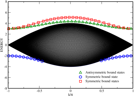
Figure 1: Energy spectrum of two fermions of the EFBH chain with periodic boundary conditions for $U=2$, $V=-3$ and $f=101$. The lines follow from numerical diagonalization of the matrix 10 and symbols are the results of analytical computations for the bound states similar to the calculations in jpnflach09PhysRevA80 .

Weight functions in normal mode space. We transform to the basis of the symmetric and antisymmetric states

$$|\Phi_{j,s}\rangle=\frac{|\Phi_{j,+}\rangle+|\Phi_{j,-}\rangle}{\sqrt{2}},\quad|\Phi_{j,a}\rangle=\frac{|\Phi_{j,+}\rangle-|\Phi_{j,-}\rangle}{\sqrt{2}}$$ (12)

where $a$ and $s$ refer to the antisymmetric and the symmetric states, respectively, $j=2,\ldots,(f+1)/2$. Note that $|\Phi_{1}\rangle$ is also a symmetric state. In this basis the matrix (10) decomposes into two irreducible parts given by

$$H^{s}(i,j)=-\left(\begin{array}[]{ccccccc}U&q\sqrt{2}&&&&\\ q^{*}\sqrt{2}&V&q&&&\\ &q^{*}&0&q&&\\ &&\ddots&\ddots&\ddots&\\ &&&q^{*}&0&q\\ &&&&q^{*}&p\end{array}\right),$$ (19)

and

$$H^{a}(i,j)=-\left(\begin{array}[]{cccccc}V&q&&&&\\ q^{*}&0&q&&&\\ &q^{*}&0&q&&\\ &&\ddots&\ddots&\ddots&\\ &&&q^{*}&0&q\\ &&&&q^{*}&-p\end{array}\right),$$ (26)

with $q=1+\tau$ and $p=\tau^{-(f+1)/2}+\tau^{-(f-1)/2}$. The rank of the symmetric matrix is $(f+1)/2$ and the rank of the antisymmetric matrix is $(f-1)/2$.

Our strategy is to compute an eigenstate for the interacting case, and use a weight function to expand it in the basis of the eigenstates of the noninteracting case. For this purpose we fix the Bloch momentum $k$, and choose a seed eigenstate $|\Psi_{\tilde{k}_{1}}^{0}\rangle$ of the unperturbed case with seed mode number $\tilde{k}$. Upon switching on the interaction it becomes a new eigenstate $|\Psi_{\tilde{k}_{1}}\rangle$, which will have overlap with several eigenstates of the unperturbed case. We expand the eigenfunction of the perturbed system using first order perturbation approximation:

$$|\Psi_{\tilde{k}_{1}}\rangle=|\Psi_{\tilde{k}_{1}}^{0}\rangle+\epsilon\sum_{{{k}_{1}^{\prime}}\neq\tilde{k}_{1}}\frac{\langle\Psi_{k_{1}^{\prime}}^{0}|\hat{H}_{U}+\hat{H}_{V}|\Psi_{\tilde{k}_{1}}^{0}\rangle}{{E_{\tilde{k}_{1}}^{0}}-E_{{k}_{1}^{\prime}}^{0}}|\Psi_{{k}_{1}^{\prime}}^{0}\rangle.$$ (27)

From expansion (27) it follows that the off-diagonal ($k_{1}\neq\tilde{k}_{1}$) weight function at the first order is given by :

$$C^{s}(k_{1};\tilde{k}_{1})=\frac{(2U|q|^{2}+VE_{k_{1}}^{0}E_{\tilde{k}_{1}}^{0})^{2}|\langle\Psi_{k_{1}}^{0}|\Psi_{\tilde{k}_{1}}^{0}\rangle|^{2}}{4|q|^{4}(E_{\tilde{k}_{1}}^{0}-E_{{k}_{1}}^{0})^{2}}.$$ (28)

with $|q|^{2}=2+2\cos(k)$ and $E_{k_{1}}^{0}$ and $E_{\tilde{k}_{1}}^{0}$ are the eigenenergies of the unperturbed system given by Eq. (11).

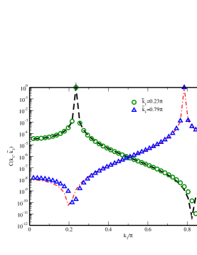
Figure 2: Weight function for two seed mode numbers $\tilde{k}_{1}=0.23\pi$ and $\tilde{k}_{1}=0.79\pi$, with the onsite and intersite interaction parameters $U=0.1$ and $V=0.08$. Here $k=0.5\pi$ and $f=101$. Dashed lines are the results using formula (28)

Symmetric states. First we consider the case of small interaction constants and as expected we find localization in normal mode space. For instance, in the case of dominant onsite interaction constant $U=1$ and $V=0.1$, quite similar results to those obtained in Ref. NguenangPRB75 are derived and the result of the perturbation formula (28) matches pretty well with those of the diagonalization procedure.

But if now we take interaction constants $U,V$ with comparable values (but again in perturbative limit) one will unavoidable deal with additional antiresonance structure presented in Fig. 2, where the weight function vanishes exactly. The appearance of these structures follows from the analytical formula (28). Indeed, in perturbative limit of interaction constants one can find such a seed $\tilde{k}_{1}$ and probe $k_{1}$ wavenumbers that the weight function becomes exactly zero. We find the following condition for zero weight:

$$\frac{U}{V}=-2\cos(k_{1})cos(\tilde{k}_{1})\;$$ (29)

It also follows from eq. (29) that there is a critical wave number given by

$$k_{1}^{c}=arcos(-\frac{U}{2V})\;.$$ (30)

An antiresonance appears only if the following inequalities are satisfied: $\pi-k_{1}^{c}<\tilde{k}_{1}<k_{1}^{c}$ (here for simplicity we assume both interaction constants positive). As it is seen from Fig. 2 the perturbative limit (28) works well even in case of presence of an antiresonance. Equation (29) further tells that an antiresonance will be observed even for $U=0$. In this case the seed wavenumber $\tilde{k}_{1}=\pi/2$ is not modified by interaction $V$. On the other hand if $V=0$ the antiresonances are not observable.

For larger values of interaction constants the perturbative predictions will get significant corrections. To show this we plot three dimensional graphs of weight function versus seed $\tilde{k}_{1}$ and probe $k_{1}$ wave numbers for various values of interaction constants in Fig. 3. As seen for small values of interaction constants the track of the antiresonances keeps the symmetry in the seed-probe mode number space traces predicted by perturbation theory. However for large interaction constants this symmetry is lost.

Antisymmetric states. The structure of the antisymmetric matrix (26) suggests that the weight function for antisymmetric states can be computed as:

$$C^{a}(k_{1};\tilde{k}_{1})=\frac{V^{2}|\langle\Psi_{k_{1}}^{0}|\Psi_{\tilde{k}_{1}}^{0}\rangle|^{2}}{(E_{\tilde{k}_{1}}^{0}-E_{{k}_{1}}^{0})^{2}}.$$ (31)

and according to this formula the weight function does not develop antiresonances. This has been confirmed by numerical diagonalization.

Discussions. Let us discuss the meaning of the observed antiresonances. Two particles, when travelling along the lattice, will meet, interact, and scatter. If prepared in an initial symmetric noninteracting seed state, the particles will scatter into all other available noninteracting symmetric states - except for one special. This is because the scattering can go either via the onsite interaction $U$ or via the intersite interaction $V$. A corresponding destructive interference makes the amplitude in this particular scattering state exactly zero. Antisymmetric states have strict zero occupation on the same site, and therefore only one scattering path (using $V$) is left. Consequently they do not show antiresonances. But they will, if we add even more distant (e.g. next-to-nearest-neighbor) interactions.

Acknowledgments J-P. Nguenang and R. Khomeriki acknowledge the warm hospitality of the Max Planck Institute for the Physics of Complex Systems in Dresden.

.

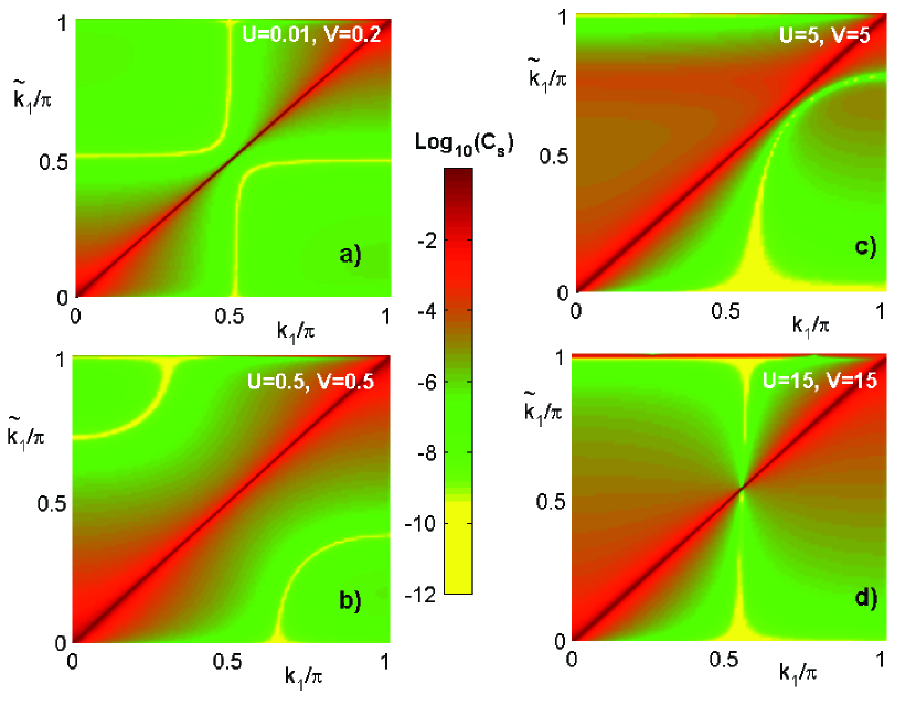
Figure 3: Three dimensional plots of the weight function for symmetric states for a fixed value of the Bloch wavenumber $k=0.12\pi$ and different interaction constants $U$ and $V$. The lattice size is the same $f=101$ as in the previous plots.

References

(1) K. Southwell, Nature 416, 205 (2002).
(2) F. Dalfogo, S. Giorgini, L. Pitaevskii, S. Stringari,
Rev. Mod. Phys. 71, 463(1999).
(3) A. Leggett, Rev. Mod. Phys. 73, 307 (2001).
(4)
L. Pitaevskii, S. Stringari, Bose-Eistein Condensation, Oxford
University Press, Oxford, 2003
(5) C. Pethick, H. Smith, Bose Eistein Condenstation in Dilute Gases,
Cambrige University Press, Cambridge, 2001
(6)
O. Mendel, M. Greiner, A. Widera, T. Rom, T.W. Hansch and I.
Bloch, Nature 425, 937 (2003)
(7) V. Fleurov, Chaos 13, 676 (2003).
(8) A.C. Scott, Nonlinear Science (Oxford University Press, Oxford, 1999).
(9) R.A. Pinto and S. Flach, Phys. Rev. A 73,022717 (2006).
(10)
R.A. Pinto and S. Flach, Europhys. Lett. 79, 66002 (2007).
(11)
R.A. Pinto and S. Flach, Phys. Rev. B 77, 024308 (2008).
(12)
A.C. Scott, J.C. Eilbeck and H. Gilhøj, Physica D 78, 194
(1994).
(13)
V. Pouthier, Phys. Rev. E 68, 021909 (2003).
(14)
J. Dorignac, J.C. Eilbeck, M. Salerno, and A.C. Scott, Phys. Rev.
Lett. 93, 025504 (2004).
(15)
J.P. Nguenang, R.A. Pinto, S.Flach. Phys. Rev. B 75, 214303
(2007).
R.A. Pinto, J.P. Nguenang, S. Flach. Physica D 238, 581 (2009).
(16)
J.P. Nguenang and S. Flach. Phys. Rev. A 80, 015601 (2009).
(17)
M.Valiente and D.Petrosyan, J. Phys. B. At. Mol. Opt. Phys.
41, 161002, (2008).