Random, thermodynamic and inverse first order transitions in the Blume-Capel spin-glass

Abstract

The spherical mean field approximation of a spin-$1$ model with $p$-body quenched disordered interaction is investigated. Depending on temperature and chemical potential the system is found in a paramagnetic or in a glassy phase and the transition between these phases can be of different nature. In given conditions inverse freezing occurs. As $p=2$ the glassy phase is replica symmetric and the transition is always continuous in the phase diagram. For $p>2$ the exact solution for the glassy phase is obtained by the one step replica symmetry breaking Ansatz. Different scenarios arise for both the dynamic and the thermodynamic transitions. These include (i) the usual random first order transition (Kauzmann-like) preceded by a dynamic transition, typical of mean-field glasses, (ii) a thermodynamic first order transition with phase coexistence and latent heat and (iii) a regime of inversion of static and dynamic transition lines. In the latter case a thermodynamic stable glassy phase, with zero configurational entropy, is dynamically accessible from the paramagnetic phase. Crossover between different transition regimes are analyzed by means of Replica Symmetry Breaking theory and a detailed study of the complexity and of the stability of the static solution is performed throughout the space of external thermodynamic parameters.

1 Introduction

In macromolecular compounds in solution, complex molecules or polymeric chains can fold into practically inactive conformations, displaying a negligible interaction with the surrounding system. The presence of inactive components can induce the existence of a fluid phase at a temperature below the temperature range at which the system is in a solid phase (crystalline, semi-crystalline or amorphous, depending on the degree of frustration) [1, 2, 3]. This corresponds to the occurrence of an inverse transition, else said ”melting upon cooling”, that is a reversible transition between a completely disordered isotropic fluid phase and a solid phase whose entropic content is greater than the entropy of the fluid.

This effect can be reproduced and studied in statistical mechanical models on a lattice with bosonic spin-$1$ variables, where the holes $s=0$ play the role of inactive states. In these models the fluid phase is the paramagnet and the solid phase is either a ferromagnet (no or weak disorder) or a spin-glass (strong disorder). A prototype model with two-body interactions between bosonic spins is the Blume-Emery-Griffiths (BEG) model with ferromagnetic interaction [4, 5, 6, 7] and its random magnetic implementation [8, 9, 10, 11, 12, 13, 14, 15, 16, 17, 18, 19, 20].

In presence of quenched disorder the random BEG model is known to display both a continuous paramagnet/spin-glass phase transition and a first order one. First order in the thermodynamic sense, i.e., with latent heat and a region of phase coexistence. Furthermore, inverse freezing takes place, with a spin-glass at high $T$ and paramagnet at low $T$. These properties have been observed in the mean-field approximation [20], where the self-consistent solution for the spin-glass phase is computed in the full Replica Symmetry Breaking (RSB) Parisi Ansatz [21, 22, 23], and on the cubic 3D lattice with nearest-neighbor couplings in systems exchanging two-body interaction, as well [24, 25]. The frustrated BEG model has been studied, as well, by means of numerical renormalization group techniques with apparently different results: on the Migdal-Kadanoff hierarchical lattice in 3D, it displays no inversion in the transition, nor a low $T$ discontinuity [26], whereas on the Wheatstone-bridge hierarchical lattice in dimension $\log 12/\log 2\simeq 3.585$ the inversion seems to be there [27].

Mean-field spin-glass models with more than two-spin interactions, called $p$-spin models, are known to yield the so-called random first order transition, i.e., a phase transition across which no internal energy discontinuity occurs but the order parameter (the Edwards-Anderson overlap $q_{\rm EA}$) jumps from zero to a finite value. Their glassy phase is described by an Ansatz with one RSB. The thermodynamic transition is preceded (in a cooling procedure) by a dynamic transition due to the onset of a very large number of metastable states separated by high barriers. The phenomenology of the $p$-spin spin-glass systems is, in many respects, very similar to the one of structural glasses [28, 35]. These models are, therefore, sometimes called mean-field glasses.

“Very large” means that the number of states ${\cal N}$ grows exponentially with the size $N$ of the system: ${\cal N}\sim\exp\Sigma N$, where the coefficient $\Sigma$ is the configurational entropy, else called complexity in the framework of quenched disordered systems. This is a fundamental property both in mean-field systems [28, 29, 30, 31, 32] and out of the range of validity of mean-field theory, e.g., in computer glass models [33, 34], or, indirectly, by measuring the excess entropy of glasses in experiments, see, e.g., [35] and references there in.

“High barriers” means that the free energy difference between a local minimum in the free energy functional of the configurational space (else called free energy landscape) and a nearby maximum (or saddle) grows with $N$. That is, it diverges in the thermodynamic limit. This is a specific artifact of mean-field glasses. The thus induced dynamic transition corresponds to the transition predicted by another mean-field theory for the dynamics of supercooled liquids: the mode coupling theory [36]. The thermodynamic transition occurring at a lower temperature is, instead, the mean-field equivalent of the so-called Kauzmann transition in glasses, else known as ideal glass transition, predicted by Gibbs and Di Marzio [37].

What happens to mean-field glasses when model features belonging to systems undergoing inverse freezing are introduced? The mean-field $p$-spin models are built either using discrete Ising variables [38, 39], soft spins [28] or spherical spins [30], the latter two being approximation of Ising discrete variables that allow for an easier analytic treatment.

In this work, we are interested in studying what happens when we mix the ingredients leading to an inverse transition (the hole state) and to a random first order transition ($p$-spin interaction), i.e., to provide a mean-field theory for inverse freezing between fluid and structural glass. We will see how, in this investigation, non-trivial features will arise, among which the inversion of dynamic and static transition and the consequent possibility of accessing low energy glassy states without running into dynamic arrest.

2 Model

The model Hamiltonian that we will consider, derives from

$${\cal H}=-\sum_{i_{1}<\ldots<i_{p}}J_{i_{1}\ldots i_{p}}s_{i_{1}}\ldots s_{i_{p}}+D\sum_{i}s_{i}^{2}$$ (1)

with $s_{i}=1,0,-1$. The couplings $J$ are Gaussian independent identically distributed variables with probability distributon:

$$P(J_{i_{1}\ldots i_{p}})=\sqrt{\frac{N^{p-1}}{\pi J^{2}p!}}\exp\left\{-\frac{N^{p-1}J_{i_{1}\ldots i_{p}}}{J^{2}p!}\right\}$$ (2)

The coefficient $D$, known as crystal field in Blume Capel (BC) models [4, 5], plays the role of a chemical potential for the empty sites (holes).

The $p=2$ case was introduced in Ref. [8] and it has been studied subsequently throughout the years [9, 10, 11, 12, 13, 14, 15, 16, 17, 18, 19, 20]. A preliminary study of the $p$-body case was presented in Ref. [40].

The spin-$1$ case can be translated into an Ising spin problem on lattice gas. Indeed, if we rewrite $s_{i}=\sigma_{i}n_{i}$ and crystal field $D=D^{\prime}+T\log 2$, with $\sigma=\pm 1$ and $n=0,1$ we have

$${\cal H}=-\sum_{i_{1}<\ldots<i_{p}}J_{i_{1}\ldots i_{p}}\sigma_{i_{1}}\ldots\sigma_{i_{p}}n_{i_{1}}\ldots n_{i_{p}}+(D^{\prime}-T\log 2)\sum_{i}n_{i}$$ (3)

We stress that the shift in chemical potential is necessary to keep the relative degeneracy of zero and non zero values of the spins in the partition sum [41]. A different shift in $D$ (or none) would, actually, define another model. Generally speaking a chemical potential transformation of the kind $D=D^{\prime}-T\log 2r$ will provide the Ising spin on lattice gas model corresponding to a model with spin$-1$ variables taking values $s=1$ (or $s=-1$) $r$ times more frequently than value $0$. E.g., $r=1/2$ corresponds to $s=1,0,0,-1$; $r=1$ to the original case $s=1,0,-1$, cf. , Eq. (3); $r=4$ to $s=1,1,0,-1,-1$ and so on [6]. In the following we will address the variants with generic $r$, as well.

In the Ising $p$-spin model, as $p>2$, besides a random first order transition (RFOT) between a paramagnet and a spin-glass phase in the 1RSB Ansatz, also a lower temperature phase transition is expected to occur between the latter and a full RSB spin-glass phase. Indeed, this is what is known to occur in the $D\to-\infty$ limit [39]. Since we are exclusively interested in the transition between fluid and (mean-field) glass, thus 1RSB stable, we can simplify the computation by approximating the discrete spins with continuous real variables satisfying a global spherical constraint.

As suggested in Ref. [42], we introduce, to this aim, the variable $\tau=\sigma(2n-1)=\pm 1$, such that $n=(\sigma\tau+1)/2$, and eventually obtain the model Hamiltonian:

$${\cal H}=-\frac{1}{2^{p}}\sum_{i_{1}<\ldots<i_{p}}J_{i_{1}\ldots i_{p}}(\sigma_{i_{1}}+\tau_{i_{1}})\ldots(\sigma_{i_{p}}+\tau_{i_{p}})+(D-T\log 2)\sum_{i=1}^{N}\frac{\sigma_{i}\tau_{i}+1}{2}$$ (4)

with

$$\sum_{i=1}^{N}\sigma_{i}^{2}=\sum_{i=1}^{N}\tau_{i}^{2}=N.$$ (5)

Applying RSB theory [21, 22, 23] we are going to investigate thermodynamics and complexity of the disordered model represented in Eq. (4).

3 Replicated free energy and order parameters

The replicated free energy, averaged over the distribution of disordered couplings, reads:

$$f_{n} = -\frac{1}{nN\beta}\log\int{\cal D}{\bm{Q}}{\cal D}{\bm{T}}{\cal D}{\bm{R}}\quad\exp\left\{-nN\beta G(\beta,D;{\bm{Q}},{\bm{T}},{\bm{R}})\right\}$$ (6)

$$-n\beta G = -(\beta D-\log 2)\sum_{a}\frac{R_{aa}+1}{2}+\frac{\beta^{2}}{4^{(p+1)}}\sum_{ab}\left(Q_{ab}+T_{ab}+2R_{ab}\right)^{p}+$$

$$+\frac{1}{2}\ln\det\left(\frac{1}{2}({\bm{QT}}+{\bm{TQ}})-{\bm{R}}^{2}\right)+\frac{n}{2}\log\pi+n,$$

$${\cal D}{\bm{Q}}=\prod_{a<b}^{1,n}dQ_{ab}\qquad{\cal D}{\bm{T}}=\prod_{a<b}^{1,n}T_{ab}\qquad{\cal D}{\bm{R}}=\prod_{a\leq b}^{1,n}R_{ab}$$

where we have inserted the three overlap matrices

$$NQ_{ab}=\sum_{i}\sigma_{i}^{a}\sigma_{i}^{b},\qquad NT_{ab}=\sum_{i}\tau_{i}^{a}\tau_{i}^{b},\qquad NR_{ab}=\sum_{i}\sigma_{i}^{a}\tau_{i}^{b}$$ (7)

and, consequently, integrated over the spin variables. The saddle point, self-consistency, equations are:

$$Q_{ab}=T_{ab}=R_{ab},\quad a\neq b$$ (8)

$$-\frac{1}{2}\left[\left({\bm{Q}}{\bm{T}}-{\bm{R}}^{2}\right)^{-1}R\right]_{ab}=\frac{\beta D-\log 2}{4}\delta_{ab}-\frac{p\beta^{2}}{2^{p+3}}\left(Q_{ab}+R_{ab}\right)^{p-1}$$ (9)

From the free energy, cf. Eq. (6), in the zero replica limit

$$f=\lim_{n\to 0}G(\beta,D,{\bm{Q}}^{\rm sp},\bm{T}^{\rm sp},\bm{R}^{\rm sp})$$ (10)

one derives all thermodynamic quantities, such as the density of filled-in sites

$$d=\frac{df}{dD}=\lim_{n\rightarrow 0}\frac{1}{n}\sum_{a}\frac{R_{aa}+1}{2};$$ (11)

the internal energy

$$u=\frac{d\beta f}{d\beta}=-Dd-\lim_{n\rightarrow 0}\frac{2\beta}{4^{(p+1)}}\frac{1}{n}\sum_{ab}\left(Q_{ab}+T_{ab}+2R_{ab}\right)^{p}$$ (12)

and the entropy

$$s = d\log 2+\frac{1}{2}\log\pi+1$$ (13)

$$+\lim_{n\rightarrow 0}\frac{1}{2n}\left[\frac{2\beta^{2}}{4^{(p+1)}}\sum_{ab}\left(Q_{ab}+T_{ab}+2R_{ab}\right)^{p}+\ln\det\left(\bm{QT}-\bm{R}^{2}\right)\right].$$

In order to compute the above expressions the precise shape of matrices $Q$, $T$ and $R$ has to be identified. There is no a priori method to deduce the correct form and one has to resort to an Ansatz.

The simplest one is the Replica Symmetric (RS) Ansatz, where the discrete symmetry group $S_{n}$, of permutation between replicas, holds for all two-indeces quantities. This means that the elements of each overlap matrix $M$ only take one value $y$ outside the diagonal and $M$ can be parametrized as:

$$M_{ab}=(M_{d}-M_{0})\delta_{ab}+M_{0},$$ (14)

where $\delta$ is the Kronecker delta. Replica symmetry always holds for one index parameters, because physical properties of a single replica must be identical for each replica. Indeed, all single index quantities, like the diagonal part of the $R$ overlap matrix, are index independent.

RS is not always self-consistent, though. Studying the fluctuations in the space of replica matrices around a RS solution for Eqs. (8)-(9) one finds that, for $p>2$, the glassy solution is not stable and one has to break the symmetry between replicas in order to find a self-consistent solution. To perform such stability analysis one needs the Hessian matrix. For our model it is computed in detail in A. We will later report about the stability analysis of both the $p=2$ case and the $p>2$. Breaking the Replica Symmetry means to allow for different values in the off-diagonal elements of the overlap matrices. The symmetry can be broken step by step allowing a further overlap value at each step and organizing replicas in clusters with a hierarchical structure [21, 22]. For our purpose one step turns out to be sufficient, leading to a one step Replica Symmetry Breaking (1RSB) solution, in which a generic matrix takes the form:

$$M_{ab}=(M_{d}-M_{1})\delta_{ab}+(M_{1}-M_{0})\epsilon_{ab}+M_{0},$$ (15)

where $\epsilon_{ab}=1$ if $a$ and $b$ belong to the same cluster of size $m$ and $\epsilon_{ab}=0$ otherwise.

4 Thermodynamics for $p=2$. Inverse freezing.

For $p=2$ the free energy evaluated in the RS Ansatz reads:

$$-2\beta\lim_{n\rightarrow 0}G^{RS}=-2(\beta D-\log 2)d+\frac{\beta^{2}}{2}(d^{2}-q^{2})+\frac{q}{\eta}+\log(\theta\eta)+\log(4\pi)+2$$ (16)

where $\theta=1-d$ and $\eta=d-q$ are eigenvalues of the matrix $QT-R^{2}=Q^{2}-R^{2}$. Self-consistency equations read:

$$\beta^{2}q = \frac{q}{\eta^{2}}$$ (17)

$$\beta^{2}\eta = \frac{\eta-\theta}{\theta\eta}+2(\beta D-\log 2)$$ (18)

The RS solution turns out to be marginally stable with respect to fluctuations in the space of replica parameters, as shown in B. In particular the lowest relevant eigenvalues of the Hessian, the so-called replicon, cf. Eq. (66), is $\Lambda_{1}^{(1)}=0$.

The self-consistency equation (17) admits $q=0$ as a solution. This leads to a paramagnetic phase, characterized by a density $d_{PM}$, determined imposing equation (18) and with a free-energy:

$$-\beta f^{RS}_{PM}(\beta,D) = -(\beta D-\log 2)d_{PM}+\frac{\beta^{2}}{4}d_{PM}^{2}+$$ (19)

$$+\frac{1}{2}\log[(1-d_{PM})d_{PM}]+\frac{1}{2}\log(4\pi)+1$$

For low $T$ and $D$ the paramagnetic phase turns out to be unstable, in particular Eq. (66) becomes negative and a new solution to Eqs. (17)-(18) occurs with $q>0$:

$$d(T,D) = 1-\frac{T}{2(1-D+T\log 2)}$$ (20)

$$q(T,D) = 1-T~{}\frac{\frac{3}{2}-D+T\log 2}{1-D+T\log 2}.$$ (21)

This SG solution is stable in the RS Ansatz in the whole region of the phase diagram where it exists, delimited by the transition line:

$$D_{c}(T)=1+T\log 2-\frac{T}{2(1-T)}.$$ (22)

In Fig. 1 we plot the phase diagram for the model. At the transition the overlap parameter $q$ grows continuously from $0$, the paramagnetic and the spin-glass solutions coincide and the density crosses continuously the transition, as shown in Fig. 2. This defines a second order transition, without latent heat or discontinuities in first order derivatives. As shown in the figure, a reentrance of the transition line points out the presence of inverse freezing.

Figure 1: $T,D$ phase diagram of the $p=2$ model case. Inset: the same diagram is shown for models with different values or the parameter $r=1,2,4,8$, ratio of the number of non-zero to zero values for the spin in the discrete counterpart of our spherical model. As $r$ increases the inverse transition region is enhanced.

Figure 2: Density behavior at $T=0.4$ across the SG/PM transition for the $p=2$ model. The paramagnetic density is shown (as a thin curve) also in its unstable phase.

As we mentioned above, in Sec. 2, one can easily switch model using Schupper-Shnerb variables [6, 7] controlling the degeneracy ratio $r$ between filled and empty sites in the original model with discrete variables. The effect of increasing $r$ is to increase the breadth of the interval in chemical potential for which inverse freezing takes place. In the inset of Fig. 1 we show the phase diagrams for some choices of $r$.

Finally, we stress that, besides $\Lambda_{1}^{(1)}$, cf. Eq. (66), there are six more distinct eigenvalues of the stability Hessian, four of which are strictly real and positive. The other two, due to the $n\to 0$ limit, can be complex conjugated and develop an imaginary part. Their real part is always positive. We refer to B, for a detailed discussion. Here we only stress that, since the RS solution is exact for $p=2$, the onset of imaginary eigenvalues is not a signature of lack of consistency of the replica Ansatz but an artifact due to the limit $n\to 0$ in the replica calculation. In Figure 3 we plot the regions of the phase diagram in which imaginary stability eigenvalues occur.

Figure 3: $T$, $D$ phase diagram: in the inner region between at least one couple of complex eigenvalues is present in the Hessian in the space of replica fluctuations, as computed on the RS solution. In the other regions all eigenvalues are real.

4.1 Random matrix approach

To conclude the analysis of the $p=2$ model we mention that, as shown in Refs. [42, 43, 44], the thermodynamics can be computed also with the method applied by Kosterlitz, Thouless and Jones [45] to the spherical Sherrington-Kirkpatrick model, that is the $D\to-\infty$ limit of the present model. The method consists in describing the model in terms of the variables $\hat{\sigma}_{i}^{\lambda}$ diagonalizing the interaction matrix:

$$\sum_{j}J_{ij}\hat{\sigma}_{j}^{\lambda}=J_{\lambda}\hat{\sigma}_{i}^{\lambda}$$ (23)

The partition function turns out to be:

$$Z=\int dz\quad\pi^{\frac{N}{2}}e^{N\left\{\frac{\beta}{2}(2z+D-T\log 2)-\log\frac{\beta}{2}-\frac{1}{2N}\sum_{\lambda}\log[\Lambda_{1}(z)\Lambda_{2}(z)]\right\}}.$$ (24)

where:

$$\Lambda_{1}(z) = \frac{\beta}{2}\left(z-\frac{J_{\lambda}}{2}-\frac{D-T\log 2}{2}\right)$$ (25)

$$\Lambda_{2}(z) = \frac{\beta}{2}\left(z+\frac{D-T\log 2}{2}\right).$$ (26)

In the thermodynamic limit, the sum over the eigenvalues can be evaluated as an integration having as measure Wigner’s semicircle law:

$$\frac{1}{N}\sum_{\lambda}f(\lambda)\longrightarrow\int_{-2}^{2}dJ\rho(J)f(J)=\int_{-2}^{2}dJ\frac{1}{2\pi}\sqrt{4-J}f(J)$$ (27)

Our replica calculation agrees with the result of Caiazzo et al. [42, 43, 44] .

5 Static results for $p>2$

The situation is far richer, and interesting, when more than two-body interactions among spin-variables are considered. As $p>2$, indeed, not only is the RS solution inconsistent in the SG phase (cf. stability analysis in B) but the exact one step RSB solution yields different kinds of transitions, some of which atypical in the framework of mean-field glasses. For $p>2$ the 1RSB free energy reads:

$$-\beta G^{1RSB} = -(\beta D-\log 2)d+\frac{\beta^{2}}{4}\left(d^{p}+(m-1)q_{1}^{p}\right)+$$

$$+\frac{1}{2}\left(2\log 2+\log\theta+\frac{m-1}{m}\log\eta_{0}+\frac{1}{m}\log\eta_{1}\right),$$

where we have used the expression of the eigenvalues of the $(Q^{2}-R^{2})$ matrix:

$$\theta = 1-d$$ (29)

$$\eta_{0} = d-q_{1}$$ (30)

$$\eta_{1} = d+(m-1)q_{1}-mq_{0}$$ (31)

We set $q_{0}=0$, because of the absence of an external magnetic field. Self-consistency equations read:

$$\phi(q_{1}) = \frac{q_{1}}{\eta_{0}\eta_{1}}$$ (32)

$$\phi(d)-\phi(q_{1}) = \frac{\eta_{0}-\theta}{\theta\eta_{0}}+2(\beta D-\log 2)$$ (33)

$$z(y) = \frac{2}{p}.$$ (34)

where

$$\phi(q) = \frac{p\beta^{2}}{2}q^{p-1}$$ (35)

$$y \equiv \frac{\eta_{0}}{\eta_{1}}$$ (36)

and

$$z(y)\equiv-2y\frac{1-y+\log y}{(1-y)^{2}}$$ (37)

is the Crisanti-Sommers function [30]. The analysis of the stability of the 1RSB solution is reported in Sec. 5.6 and in C.

The complexity functional, defined as the Legendre transform of the free energy functional, evaluated on the saddle point solution yielded by equations (32) and (33), logarithmically counts the number of metastable states [29]. It reads:

$$\Sigma_{LT}(m,D,\beta) = \beta m^{2}\frac{\partial}{\partial m}G(m,D,\beta,q_{1}^{\rm sp}(m,D,\beta),d^{\rm sp}(m,D,\beta))$$

$$= -\frac{m^{2}\beta^{2}\left(q_{1}^{\rm sp}\right)^{p}}{4}-\frac{m\beta q_{1}^{\rm sp}}{2\eta_{1}^{\rm sp}}-\frac{\beta}{2}\log\frac{\eta_{0}^{\rm sp}}{\eta_{1}^{\rm sp}}$$

To determine the dynamic transition line $T_{d}(D)$ one has to impose a maximal complexity (versus $m$) condition:

$$\frac{\partial\Sigma_{LT}}{\partial m}=0\qquad\leftrightarrow\qquad\eta_{1}=(p-1)\eta_{0}$$ (39)

in place Eq. (34).

From the analysis of the paramagnetic solution ($q_{0}=q_{1}=0$), solving the self-consistency equation

$$\frac{p}{2}d^{p}(1-d) = T^{2}(2d-1)+2(TD-T^{2}\log 2)(1-d)d$$ (40)

one finds a region in the $T,D$ phase diagram where three solutions for the PM density $d$ occur. One of them is always unstable, whereas the other two coexist between the spinodal lines. The latter can be expressed, in a parametric form in $d$, by

$$D=\sqrt{\frac{p}{p-1}}~{}\frac{d^{-1+p/2}\left(d+p-3dp+2d^{2}p+2(1-d)^{2}d(p-1)\ln(2r)\right)}{2(1-d)\sqrt{4d^{2}-4d+1}}$$ (41)

$$T=\sqrt{p(p-1)}~{}\frac{d^{p/2}(1-d)}{\sqrt{4d^{2}-4d+1}}$$ (42)

The first order transition line is, eventually, obtained by comparing the free energies of the two solutions $d_{\rm PM^{+}}$ and $d_{\rm PM^{-}}$.

In Figs. 4 and 5 we show the phase diagram for $p=3$, both for $r=1$ and $r=4$. For $r=1$ no reentrance of the thermodynamic transition line appears, as shown in Fig. 4, but, increasing $r$, inverse freezing is clearly reproduced, cf. Fig. 5. The first order PM^-/PM⁺ line is the thick-dotted line and spinodal lines are plotted as thin-dotted lines. Qualitatively distinct transition regimes are identified. We will dedicate a subsection to each one of them, starting from the most conventional one. As a reference we follow the phase diagram in Fig. 4 moving from small (and negative) to large (positive) values of the chemical potential of the holes.

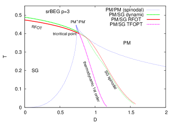
Figure 4: $T$,$D$ phase diagram of the spherical $p=3$-spin BC model with filled-in to empty sites ratio $r=1$.

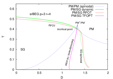
Figure 5: $T$,$D$ phase diagram of the spherical $p=3$-spin BC model with filled-in to empty sites ratio $r=4$. A reentrance occurs in the first order thermodynamic transition line.

5.1 Random First Order Transition (RFOT)

For $D$ small enough our model displays the same behaviour as the spherical $p$-spin model [30] and is an example of the well know RFOT. At high temperature the system is in a ergodic paramagnetic phase. As it is cooled down, crossing a temperature $T_{d}$ it undergoes a dynamical arrest, despite the static order parameter $q_{1}$ is still null. Only at a lower temperature $T_{s}<T_{d}$ a thermodynamic phase transition occurs. Critical static and dynamic lines are determined solving the equation systems (32), (33), (34) or (32), (33), (39), respectively. For $p=3$, $r=1$, e.g., in the $D,T$ phase diagram they read

$$D_{s}(T) = \frac{1.8794T^{1/3}-2.49052T-0.989769T^{5/3}}{1-1.42793T^{2/3}}$$ (43)

$$D_{d}(T) = \frac{21.6337T^{1/3}-27.6822T-11.5344T^{5/3}}{12.-16.6407T^{2/3}}$$ (44)

These curves are the $m=1$-lines for statics and dynamics, respectively represented in Figs. 4, 5 by the thick full (dark grey) and dashed (light grey) lines. As one can observe in Fig. 6, crossing the dynamical temperature from high $T$ values, a collection of high complexity SG states arise at high free energy values. Each one of these states has a free-energy strictly greater than the free energy of the equilibrium state, namely the paramagnetic one. Indeed, from a strictly thermodynamic point of view, the stable state is the paramagnetic one, leaving each SG state as metastable. Decreasing further the temperature the system gains new states with lower free-energy and complexity, until, at $T=T_{s}$, zero-complexity SG states appear, which turn out to yield the stable SG phase.

Figure 6: $\Sigma(f;T,D=0)$ in a region of temperature around static random first order ($T_{s}(D=0)=0.4739$) and dynamic ($T_{d}(D=0)=0.4892$) transition.

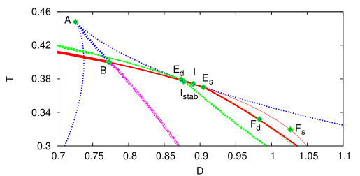
Figure 7: Detail of the $D,T$ phase diagram with $r=1$ with all significant critical points. $A$ is the critical point of the PM⁺/PM^- transition; $B$ is the merging point of the first order PM⁺/PM^- with the first order SG/PM^- line; $E_{d,s}$ is the limit of stability of the SG (dynamic/static) solution along the $m_{d,s}=1$ line; $I$ is the point of dynamic-static inversion of the $m=1$ lines (where the 1RSB solution is unstable) and $I_{\rm stab}$ is the point of dynamic-static inversion in which the SG solution is stable; $F_{d,s}$ are the points of dynamic-dynamic and static-static $m$-lines crossing, in the region of replica instability.

5.2 Thermodynamic First Order Phase Transition

At $(D_{A},T_{A})\simeq(0.73,0.44)$ a first order transition line starts developing in the PM phase, separating two distinct PM phases as $T$ is lowered. The two phases are caracterized by their density, which has a jump crossing the transition line. We name PM^± the paramagnetic phase at higher/lower density. At $(D_{B},T_{B})\simeq(0.77,0.40)$ the first order PM⁺/PM^- transition line merges with a first order SG/PM^- transition line $D_{c}(T)$, cf. Fig. 7, and the thermodynamic transition to the SG is not ”random” anymore but, rather, a standard first order, ruled by the Clausius-Clapeyron equation, cf., e.g., Ref. [20].

Figure 8: Free energy in the SG and PM phases in qualitatively different scenarios. The full curve represents $\Phi_{\rm SG}$ in the 1RSB Ansatz , $\Phi_{\mbox{PM}^{+}}$ and $\Phi_{\mbox{PM}^{-}}$ vs. $T$ are plotted as dashed curves. $D=0.7,0.75,0.8,0.9$. Top left: at $D=0.7<D_{A}$, RFOT between PM^- and SG, at $T_{s}$. Top right: RFOT between PM⁺ and SG, at $T_{s}$, and TFOT between PM^- and PM⁺, at $T_{c}$, for $D=0.75$ (larger than $D_{A}$ and smaller than $D_{B}$). Bottom left: TFOT between PM^- and SG, at $T_{c}$, and RFOT between PM⁺ and metastable SG, at $T_{s}$. Bottom right: RFOT between PM⁺ and metastable SG, at $T_{s}$.

The SG solution departs from the high-density PM⁺ phase, i.e., SG and PM⁺ belong to the same saddle point of Eq. (5), see, e.g., Fig. 8. For chemical potential values $D<D_{B}$ the thermodynamic transition to the SG is still the RFOT analyzed above. In Fig. 8 we plot the temperature behavior of the free energies of the PM^-, PM⁺ and SG phases in three qualitatively different cases: for $D<D_{A}$, $D_{A}<D<D_{B}$ and $D>D_{B}$.

Figure 9: Left: Latent heat at the first order transition at $D=1$ for the case $r=1$. Inset: discontinuity of overlap $q_{1}$ (dotted line) and density $d$ (dashed line) across the same transition point at $T_{c}=0.142$. Right: Latent heat at $D=1.2$ for the case $r=4$, in presence of inverse freezing the SG phase transforms into the PM (at lower entropy $\Delta s=s_{\rm SG}-s_{\rm PM}>0$) one as $T$ decreases, taking heat from the thermal bath. Inset: the overlap $q_{1}$ (dotted line) is different from zero above the critical temperature $T_{c}=0.146$. The density $d$ (dashed line) decreases discontinuously in the low $T$ PM phase.

Along the $D_{c}(T)$ transition line, latent heat is taken from the glass in order to be transformed into a paramagnet, as we show in Fig. 9.

Around that line the SG and the PM phases coexist and compete. Beyond the B point, the RFOT line $T_{s}(D)$ becomes the SG spinodal since on the right side of the $D_{c}(T)$ line the glassy phase is metastable with respect the PM one. That is, the whole hierarchy of global and local glassy minima lies above the global thermodynamically dominant PM minimum in the free energy landscape: $\Phi_{SG}>\Phi_{PM}$.

This might seem weird in some respect. Indeed, in RSB theory, e.g., in the spherical $p$-spin model, the 1RSB SG solution stems out of the PM phase, which is RS. At a given $T_{s}$ a 1RSB solution appears with a discontinuous jump in $q_{\rm EA}$ and no discontinuity in the free energy. As $T<T_{s}$, the SG free energy is larger than the PM free energy but it is the one thermodynamically stable because of the $n-1$, $n-m$ or $m-1$ factors present in the free energy expression Eq. (5) whose sign is inverted in the $n\to 0$ limit. This implies that looking for a minimal free energy at finite integer number of replicas corresponds to look for the maximal of the Parisi free energy. In our case, in fact, the SG 1RSB phase stems out of a PM (PM⁺) phase, as shown in Fig. 8. However, it competes with another phase PM^-, corresponding to a different saddle point of Eqs. (5), that does not transform into a SG and whose free energy does not involve overlap terms and, consequently, coefficients do not change sign in the replica calculation.

As a homogeneous selecting rule, we can, thus, apply the minimal free-energy principle for all competing solutions with $n>1$ and let $n\to 0$ only after the choice of the dominant stable phase has been done. To better exemplify this, we plot in Fig. 10 the RS approximated SG solution at finite $n$ for different values of $n$ and we compare it with both the free energies of PM^- and PM⁺. For $n>1$ the free energy of the SG RS solution crosses the PM^- free energy for $T$ lower than the transition temperature between the two PM phases, signaling the presence of a transition between the PM^- and the SG. The dominant phase is the one of least free energy, i.e., the SG phase. As $n$ decreases the critical temperature decreases until, for $n=1$, the SG free energy turns equal to the PM⁺ one. As $n<1$ the SG free energy shifts further towards small temperature but the thermodynamic order relationship with the free energy of the PM^- phase is unchanged. Breaking the replica symmetry on the same SG phase leads to a higher free energy and shifts the first order critical temperature towards smaller $T$. This does not affect the order relationship with respect to the other self-consistent solution, i.e., the PM^- phase.

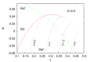
Figure 10: Analysis of free energy in temperature at finite $n=0,0.5,1,1,5,2$ in the RS approximation. The full curve is the SG solution in the zero replica limit. The dashed curves are finite $n$ SG solutions. For $n=1$ the SG free energy coincides with the PM⁺ free energy. Each one of the SG curves crosses the free energy curve of the PM^- phase signaling a first order phase transition between the PM^- phase, dominant at high $T$ and the SG phase (dominant at low $T$). Since the SG free energy is computed in the RS Ansatz, the exact free energy is a little bit larger and the crossing point at slightly smaller $T$.

5.3 Dynamic-Static inversion

As the chemical potential increases, the temperature interval between $T_{s}(D)$ and $T_{d}(D)$ decreases down to zero at $T_{s}(D_{I})=T_{d}(D_{I})=T_{I}=0.3739$, with $D_{I}=0.8905$. For larger $D$ the dynamic and static lines invert their position in $T$. Coming from high temperature, this means that the static line ($m=1$ in Eq. (34)) will be met before the dynamic one ($m=1$ in Eq. (39)). According to the behavior of the complexity this implies that the lowest equilibrium glassy states are dynamically accessible at the static transition and that excited glassy states only develop as $T$ is decreased, as displayed in Fig. 11.

Actually, it can be seen from the complete stability analysis, cf . C, that for $D>D_{E_{d}}=0.8737$, slightly smaller than $D_{I}$, the SG dynamic solution spanned along the $m=1$-line turns out to display a couple of complex conjugated eigenvalues with negative real part. This implies that for $D\geq D_{E}$ the first thermodynamically stable SG solution occurs with the static parameter $m<1$ and zero complexity for the excited states. The static-dynamic inversion then occurs, self-consistently, for values of $m<1$, at $D_{I_{\rm stab}}=0.877$, $T_{I_{\rm stab}}=0.377$.

Figure 11: $\Sigma(f)$ for $T=0.35$ at different values of $D$ below the static transition.

5.4 $m$-lines inversion, compressibility and replica stability

As one can see from Fig. 12, solving equations (32), (33) and Eq. (34) [else (39)], and following solutions at fixed $m$ in the $D,T$ plane, each $T_{m}(D)$ curve (”$m$-line”) develops a maximum and $T_{m}(D)$ lines at different $m$ values cross. This leads to an ambiguity: there is a region in the phase diagram in which in each point two different solution of Eqs. (32), (33),(34) occur. A criterium is, then, required to select the correct (metastable) phase in each point and, furthermore, a way to mark the spinodal of the SG. The solution comes from the positiveness of the compressibility $\kappa$ and from the complete analysis of the stability of the 1RSB solution in the replica space. Moreover, as we already mention, the $m$-line inversion comply with the fact that the spinodal SG lines (both dynamic and static) will cease to be a line of constant $m=1$.

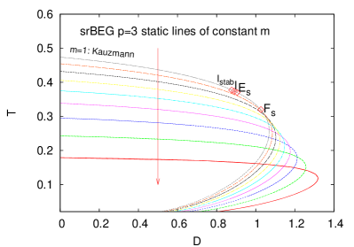
Figure 12: $T(D)$ lines of constant $m$ (from static equations). As $D$ is large enough they bend and cross each other. Left: complete behavior of $m$-lines. Right: only curves along which the compressibility is non-negative are plotted. An equivalent situation occurs for the dynamic $m$-lines. The thick continuous curve is the line where complex stability eigenvalues acquire negative real part: solutions on the right hand side of the stability line are rejected.

5.5 Compressibility

As a thermodynamic quantity the compressibility is usually defined as:

$$k=-\left.\frac{\partial\log V}{\partial p}\right|_{T}$$ (45)

In our model, where the role of the pressure is played by the chemical potential $D$ and the inverse specific volume is the density of filled-in states $d$, the compressibility reads:

$$k=d\left.\frac{\partial d^{-1}}{\partial D}\right|_{T}=-\frac{1}{d}\left.\frac{\partial d}{\partial D}\right|_{T}=-\frac{1}{d}\left.\frac{\partial d}{\partial m}\right|_{T}\left.\frac{\partial m}{\partial D}\right|_{T}$$ (46)

where the last equality comes from the Fubini’s implicit function theorem. Obviously, solutions with negative compressibility are unphysical and have to be discarded. At fixed $T$ the value $m=\hat{m}$ yielding the zero point of the compressibility is given by

$$\left.\left(\left.\frac{\partial m}{\partial D}\right|_{T}\right)\right|_{m=\hat{m}}=0$$ (47)

using, e.g., Eq. (33) for the $D(m)$ dependence. Beyond $\hat{m}(T)$ the compressibility turns negative and that solution will be rejected. This kind of ”selection rule” has to be used for both the static and the dynamic m-lines.

The positiveness of $\kappa$ is certainly a necessary condition for thermodynamic stability. On top of that we anticipate that, from the replica stability analysis, we found a small region of the phase diagram where $\kappa>0$ but the real part of a couple of complex-conjugated eigenvalues among $\Lambda_{2,1}$, or among $\Lambda_{3,1}$ of the Hessian in the replica space for the 1RSB Ansatz, cf. Eqs. (111), (126), is negative (see also the right panel of Fig. 12). The spinodal lines plotted in Figs. 4, 5 are drawn taking the latter observation into account. See also the right panel of Fig. 12

Figure 13: Compressibility vs, $T$ at $D=0.5<D_{A}$, in the RFOT regime (left) and at $D=1>D_{B}$ in the TFOT regime (right).

The previous discussion implies that the dynamic SG spinodal is the $m=1$-line on the left side of the point $F_{d}$, $(D_{F_{d}}=0.98,T_{F_{d}}=0.33)$ and a line of decreasing $m$ on the right side. Also the static SG spinodal undergo the same change at the point $F_{s}$ $(D_{F_{s}}=1.03,T_{F_{s}}=0.32)$. We remark, however, that this change in behavior arises for $D>D_{I_{\rm stab}}$, where the $m=1$-line cease to be stable in the replica space and $D>D_{I}$, after that the static-dynamic inversion occurs.

5.6 Stability of 1RSB solution

In order to determine the above phase diagram it has been necessary to study the stability of the 1RSB solution in the $T,D$ plane. In C we show the details of our analysis. The phenomenology looks similar to the RS case with both real and complex eigenvalues. The stability of the SG solution is ruled by $\Lambda_{1,1}^{(3)}$, the lowest real eigenvalue of the matrix $H_{11}$, cf. Eq. (99). Evaluated on the static SG solution it is always positive, thus, according to our analysis, the static SG 1RSB solution is always stable. If, however, the static Eq. (34) is not imposed and the parameter $m$ is, thus, left undetermined, the positiveness of $\Lambda_{1,1}^{(3)}$ is equivalent to the condition:

$$\eta_{1}>(p-1)\eta_{0}$$ (48)

and the equality $\Lambda_{1,1}^{(3)}=0$ turns out to coincide with the dynamical condition Eq. (39). The other real eigenvalues are positive in the whole phase diagram.

In the region of phase coexistence, near the SG spinodal, the stability analysis actually revelas more subtle features. Indeed, as in the $p=2$ case, cf. Sec. 4, complex eigenvalues are present and some of them develop a negative real part. In particular, solutions with negative compressibility always yield an imaginary eigenvalues with negative real part. Moreover, in a small region of the $T$,$D$ plane solutions with $\kappa\gtrsim 0$ also display complex eigenvalues, $\Lambda_{2,1}$ or $\Lambda_{3,1}$, cf. Eqs. (111), (126) with negative real part. As anticipated, in determining the phase diagram we have thus rejected solutions with negative replica eigenvalues, including all those with negative compressibility.

Figure 14: Region of complex eigenvalues in the $T,D$ plane for the $p=3$ model.

6 Conclusions

We have been analyzing, at the level of mean-field theory, a family of models mixing the properties of (i) Blume-Capel models with quenched disorder and (ii) spin-glass models with many-body ($p>2$) interactions. The first ones are known to reproduce the inverse freezing occurring, e.g., in complex macromolecular compounds in solution [1, 2, 3], and display first order thermodynamic phase transitions even in presence of strong disorder, The latter yield most of the basic features of the standard folklore of glassy systems and are often refereed to as mean-field glasses. Our aim has been to investigate to behavior of dynamic arrest, displayed in mean-field glasses, as a system undergoes an inverse thermodynamic transition.

We have been studying the problem by means of replica theory for the two qualitatively distinct cases with $p=2$ and $p>2$, both looking at the thermodynamic and at the dynamic properties. The dynamics has been tackled by means of the analysis of the complexity of the free energy landscape. The model approximation used is to pass from discrete spin-$1$ variables to spherical ones (i.e., continuous variables with an overall ”spherical” constraint) keeping the original probabilistic relationship between states of the discrete spin: $r\equiv$ $[\#$ of times $s=1]/$ $[\#$ of times $s=0]$. This allows for thoroughly analytical computation of complicated physical quantities. We have been mainly focusing on the case $r=1$, i.e., the spherical formulation of the original BC model but we have considered, as well, model cases with different $r$ values. Indeed, in those cases where the spherical analogue of the original spin-$1$ system ($r=1$) do not show inverse freezing, a simple variant of the model for larger $r$ is suitable to describe such phenomenon.

The external parameters driving possible transitions are the temperature and a chemical potential for the empty states of the spin-$1$ variables, the so-called ”crystal field” $D$. For $D=-\infty$ one has no holes and the limit of the model is the spherical spin-glass. In that limit, in the $p=2$ case [45] the spin-glass phase is described by a replica symmetric Ansatz and the transition turns out to be always continuous, whereas, as $p>2$ the RS solution is unstable and the right physics is described by a one step Replica Symmetry Breaking phase [30]. On top of it the transition is not continuous (at zero external magnetic field) in the order parameter and it is often refereed to as random first order.

In the present study we find that, for $p=2$, the situation is not very different for the original spherical spin-glass, with a spin-glass phase stable under the RS Ansatz. The only addition is the presence of a transition between competing paramagnetic phases at high $T$ ($D$) and the occurrence of inverse freezing for large enough chemical potential $D$. For $p>2$ the situation is, instead, drastically modified. Besides the standard RFOT, we find that, for large enough $D$, a first order thermodynamic phase transition between the spin-glass and the paramagnetic phase takes over, with latent heat and jumps in density and overlap order parameter. The spin-glass becomes metastable with respect to the paramagnet and the RFOT line plays the role of the spin-glass spinodal. Moreover, analyzing in detail the structure of the solutions in the phase diagram and their stability properties, we find that the spin-glass phase can be approached, in given regions, without incurring in dynamic arrest, unlike in the standard $p$-spin and that the first spin-glass solution display values of replica symmetry breaking parameter $m$ less than one. The study of the complexity functional clarify how this observation amounts to a scenario in which, in a cooling experiment, lowest glassy minima of the free energy landscape develop first and excited metastable glassy states only arise as temperature is further lowered. This provides a model case where actual dynamics might be followed along given paths of the phase diagram into the deep glassy phase without being stuck in the threshold states.

Appendix A Hessian of the spherical $p$-spin Blume-Capel model

In order to verify the stability of a saddle-point calculation, the positiveness of the fluctuation matrix evaluated on the stationary solution has to be checked. This Hessian matrix is constructed as the second order variation of the free-energy potential (6) with respect to the three overlap matrices (7) and, indeed, depends on two couples of indexes:

$$H(G)^{O,O^{\prime}}_{ab;cd}=\frac{\partial^{2}G}{\partial O_{ab}\partial O^{\prime}_{cd}},\quad O,O^{\prime}=Q,S,T,$$ (49)

In detail the elements read

$$\frac{\partial G^{2}}{\partial Q_{ab}\partial Q_{cd}} = -B_{ab}\delta_{a,c}\delta_{bd}+\frac{1}{8}\left[A_{a,c}(TAT)_{bd}+2(TA)_{a,c}(AT)_{bd}+\right.$$

$$\left.+(TAT)_{a,c}A_{bd}\right]$$

$$\frac{\partial G^{2}}{\partial Q_{ab}\partial T_{cd}} = -B_{ab}\delta_{a,c}\delta_{bd}+\frac{1}{8}\left[A_{a,c}(TAQ)_{bd}+(QA)_{ac}(AT)_{bd}+\right.$$

$$\left.+(AT)_{ac}(AQ)_{bd}+(TAQ)_{ac}A_{bd}\right]-\frac{1}{4}\left(A_{bd}\delta_{ac}+A_{ac}\delta_{bd}\right)$$

$$\frac{\partial G^{2}}{\partial Q_{ab}\partial R_{cd}} = -2B_{ab}\delta_{ac}\delta_{bd}-\frac{1}{4}\left[A_{ac}(TAR)_{bd}+(RA)_{ac}(AT)_{bd}\right.$$

$$+\left.(AT)_{ac}(AR)_{bd}+(TAR)_{ac}A_{bd}\right]$$

$$\frac{\partial G^{2}}{\partial T_{ab}\partial Q_{cd}} = -B_{ab}\delta_{ac}\delta_{bd}+\frac{1}{8}\left[A_{ac}(TAQ)_{bd}+(QA)_{ac}(AT)_{bd}+\right.$$

$$+\left.(AT)_{ac}(AQ)_{bd}+(TAQ)_{ac}A_{bd}\right]-\frac{1}{4}\left(A_{bd}\delta_{ac}+A_{ac}\delta_{bd}\right)$$

$$\frac{\partial G^{2}}{\partial T_{ab}\partial T_{cd}} = -B_{ab}\delta_{ac}\delta_{bd}+\frac{1}{8}\left[A_{ac}(QAQ)_{bd}+2(QA)_{ac}(QA)_{bd}+\right.$$

$$+ \left.(QAQ)_{ac}A_{bd}\right]$$

$$\frac{\partial G^{2}}{\partial T_{ab}\partial R_{cd}} = -2B_{ab}\delta_{ac}\delta_{bd}-\frac{1}{4}\left[A_{ac}(QAR)_{bd}+(RA)_{ac}(AQ)_{bd}\right.$$

$$+\left.(AQ)_{ac}(AR)_{bd}+(QAR)_{ac}A_{bd}\right]$$

$$\frac{\partial G^{2}}{\partial R_{ab}\partial Q_{cd}} = -2B_{ab}\delta_{ac}\delta_{bd}-\frac{1}{4}\left[A_{ac}(TAR)_{bd}+(RA)_{ac}(AT)_{bd}\right.$$

$$+\left.(AT)_{ac}(AR)_{bd}+(TAR)_{ac}A_{bd}\right]$$

$$\frac{\partial G^{2}}{\partial R_{ab}\partial T_{cd}} = -2B_{ab}\delta_{ac}\delta_{bd}-\frac{1}{4}\left[A_{ac}(QAR)_{bd}+(RA)_{ac}(AQ)_{bd}\right.$$

$$+\left.(AQ)_{ac}(AR)_{bd}+(QAR)_{ac}A_{bd}\right]$$

$$\frac{\partial G^{2}}{\partial R_{ab}\partial R_{cd}} = -4B_{ab}\delta_{ac}\delta_{bd}+\frac{1}{2}\left[A_{ac}(RAR)_{bd}+2(RA)_{ac}(AR)_{bd}+\right.$$

$$+\left.(RAR)_{ac}A_{bd}\right]+\frac{1}{2}\left(A_{bd}\delta_{ac}+A_{ac}\delta_{bd}\right)$$

where:

$$A_{ab} = (QT-R^{2})_{ab}$$ (50)

$$B_{ab} = \frac{\beta^{2}p(p-1)}{2^{6}}\left(\frac{Q_{ab}+T_{ab}+2R_{ab}}{4}\right)^{p-2}$$ (51)

To check its positiveness of the Hessian, one needs to compute, and determine the sign of all the eigenvalues of its action on fluctuation matrices ($\delta o$’s):

$$\Lambda~{}\delta o_{ab}. = \sum_{cd}\left(\frac{\partial^{2}G}{\partial O_{ab}\partial Q_{cd}}\delta q_{cd}+\frac{\partial^{2}G}{\partial O_{ab}\partial T_{cd}}\delta t_{cd}+\frac{\partial^{2}G}{\partial O_{ab}\partial R_{cd}}\delta r_{cd}\right)=$$ (52)

$$= -B_{ab}\delta o_{ab}+\frac{1}{2}\sum_{cd}\left(\sum_{O^{\prime}}\frac{\partial^{2}}{\partial O_{ab}\partial O^{\prime}_{cd}}\log|A|\right)\delta o_{cd}.$$ (53)

In order to solve Eq. (53), a set of $\frac{3n^{2}-n}{2}$ coupled equations, one needs to find a way to project the system on proper subspaces, that allows to translate the calculation to an usual eigenvalues problem.

Appendix B Stability of the RS solution

In order to understand the appearance of complex eigenvalues, we start the stability analysis retaining $n$ finite. In the RS ansatz the matix (51) becomes:

$$A_{ab}^{-1} = \frac{1}{4\theta\eta}\delta_{ab}-\frac{q}{4\theta\eta\eta_{1}}\equiv x\delta_{ab}+w$$ (56)

$$x\equiv\frac{1}{4\theta\eta}$$

$$w\equiv-\frac{1}{4\theta\eta\eta_{1}}$$

$$B_{a\neq b} = \frac{1}{32}\phi^{\prime}(q)=\frac{\beta^{2}p(p-1)}{2^{6}}q^{p-2}\equiv B_{q},$$ (57)

$$B_{a=b} = \frac{1}{32}\phi^{\prime}(d)=\frac{\beta^{2}p(p-1)}{2^{6}}d^{p-2}\equiv B_{d}$$ (58)

where $\theta=1-d$, $\eta=d-q$ and $\eta_{1}=d-(1-n)q$, with $\eta_{1}\to\eta$ if $n\to 0$. The parameter $x$ is always positive. For later convenience, we define:

$$D_{++} \equiv x^{2}(\eta+\theta)^{2};\qquad\quad\,\,\,H_{++}\equiv xw[\eta^{2}+4\theta^{2}+\eta(4\theta-\eta_{1})];$$ (59)

$$D_{+-} \equiv (\eta+\theta)(\eta-\theta);\qquad H_{+-}\equiv xw(\eta^{2}-4\theta^{2}-\eta\eta_{1});$$ (60)

$$D_{--} \equiv (\eta-\theta)^{2};\qquad\qquad\,\,\,H_{--}\equiv xw(\eta^{2}+4\theta^{2}-\eta(2\theta+\eta_{1})$$ (61)

Projection on subspace $S_{1}$

Fluctuations that involve the overlap of one replica with the others, are selected by projecting the Hessian (49) in the subspace $S_{1}$ defined by:

$$\delta r_{a,a}=0,\quad\sum_{\gamma}\delta q_{a,\gamma}=0$$

with dimension $d(S_{1})=d_{tot}-4n=\frac{3n(n-3)}{2}$. This is called replicon subspace and in $S_{1}$ the Hessian matrix reduces to:

$$\begin{array}[]{c}H_{1}=\left(\begin{array}[]{c c c}\frac{1}{2}D_{++}-B_{q}&\frac{1}{2}D_{++}-\frac{x}{2}-B_{q}&-D_{+-}-2B_{q}\\ \frac{1}{2}D_{++}-\frac{x}{2}-B_{q}&\frac{1}{2}D_{++}-B_{q}&-D_{+-}-2B_{q}\\ -D_{+-}-2B_{q}&-D_{+-}-2B_{q}&2D_{--}+x-4B_{q}\\ \end{array}\right)\end{array}$$ (62)

displaying no explicit $n$ dependence. The characteristic polynomial, evaluated on the SG solution, reads:

$$P[H_{1}] = \left(\Lambda-\frac{x}{2}\right)(\Lambda^{2}-b_{1}\Lambda+c_{1})$$ (63)

$$b_{1} = \frac{3\left(\eta^{2}-(p-2)\theta^{2}\right)}{16\eta^{2}\theta^{2}}$$ (64)

$$c_{1} = -\frac{p-2}{8\eta^{2}\theta^{2}}$$ (65)

Interaction with $p=2$

For $p=2$ $c_{1}=0$, $b_{1}>0$: two eigenvalues will be positive and one will be zero.

$$\Lambda_{1}^{(1)} = 0$$ (66)

$$\Lambda_{1}^{(2)} = \frac{3}{16\theta^{2}}>0$$ (67)

$$\Lambda_{1}^{(3)} = \frac{1}{8\theta\eta}>0$$ (68)

We have marginal stability of the RS-SG solution.

Interaction with $p>2$ and replica symmetry breaking

If $p>2$, instead, $c_{1}<0$, leading to a negative zero of the polynomial and causes the instability of the RS-SG solution. As $p>2$ one has to resort to a more complicated Ansatz, the 1RSB scheme of computation, whose stability will be analyzed in the following appendix. We now continue the analysis of the RS fluctuations in other subspaces.

Projection on subspace $S_{2}$

Fluctuations of the cluster of replicas are selected by projecting in $S_{2}$, defined as:

$$\sum_{\gamma}\delta r_{\gamma,\gamma}=0,\quad\sum_{\gamma,\delta}\delta q_{\gamma,\delta}=0$$

with $d(S_{2})=4n-4$. In $S_{2}$ the Hessian reduces to:

$$\begin{array}[]{c}H_{2}=H_{1}^{\prime}+\left(\begin{array}[]{c c c c}\frac{n-2}{8}H_{++}&\frac{n-2}{8}(H_{++}-2w)&-\frac{n-2}{4}H_{+-}&-\frac{n-2}{4}H_{+-}\\ \frac{n-2}{8}(H_{++}-2w)&\frac{n-2}{8}H_{++}&-\frac{n-2}{4}H_{+-}&-\frac{n-2}{4}H_{+-}\\ -\frac{n-2}{4}H_{+-}&-\frac{n-2}{4}H_{+-}&\frac{n-2}{2}(H_{--}+w)&\frac{n-2}{2}(H_{--}+w)\\ -\frac{1}{2}H_{+-}&-\frac{1}{2}H_{+-}&H_{--}+w&H_{--}+w\\ \end{array}\right)\end{array}$$ (74)

(75)

where:

$$H_{1}^{\prime}:=\left(\begin{array}[]{c|c}H_{1}&0\\ \hline\cr 0&\Lambda_{4}\\ \end{array}\right)$$ (76)

with

$$\Lambda_{2}^{(4)}=-4B_{d}+x+2D_{--}$$ (77)

For generic $n$, apart from $n=4$, $H_{2}$ is not symmetric, so the matrix can have complex eigenvalues. The characteristic polynomial of the $H_{2}$ matrix, evaluated on the SG solution, reads:

$$P[H_{2}](\Lambda)=\left(-\Lambda+\frac{x}{2}+\frac{n-2}{4}w\right)\left[-\Lambda^{3}+a_{2}(n)\Lambda^{2}-b_{2}(n)\Lambda+c_{2}(n)\right]$$

(78)

In the limit $n\to 0$, the coefficients are:

$$\begin{array}[]{c c c}a_{2}&=&-2w\eta^{2}x^{3}\\ b_{2}&=&-wx+6x^{4}\eta^{4}\\ c_{2}&=&5x^{2}\eta^{2}-2wx\theta^{2}\\ \end{array}$$ (79)

Interaction with $p=2$

For the case $p=2$, a numerical study ensures that all the solutions of the characteristic polynomial are real positive or complex conjugated with a positive real part. The region of the $(D,T)$ plane where the polynomial has complex zeros (shown in Fig 3) can be determined imposing:

$$\frac{u^{2}}{4}+\frac{v^{3}}{27}>0$$ (80)

where (in terms of the polynomial coefficients):

$$\begin{array}[]{c c c}u&=&\frac{2a_{2}^{3}}{27}+\frac{a_{2}b_{2}}{3}+c_{2}\\ v&=&-b_{2}-\frac{a_{2}^{2}}{3}\end{array}$$ (81)

Stability of the paramagnetic phase

In the paramagnetic phase $w\propto q=0$, implying $H_{\pm\pm}=0$, cf. Eqs. (59)- (61) and the Hessian simplifies as $H_{2}=H_{1}^{\prime}$. Its characteristic polynomial is:

$$P[H_{2}]=(\Lambda-\Lambda_{4})\left(\Lambda-\frac{x}{2}\right)(-\Lambda^{2}-b_{2}\Lambda+c_{2})$$ (82)

where now, cf. Eq. (63):

$$b_{2} =\frac{3}{16}\left(\frac{2d^{2}-2d+1}{(1-d)^{2}d^{2}}-\beta^{2}\delta_{p}^{2}\right)$$ (83)

$$c_{2} =\frac{1-\beta^{2}d^{2}\delta_{p}^{2}}{32(1-d)^{2}d^{2}}$$ (84)

Its zeros are:

$$\Lambda_{1}^{(2)} = \frac{x}{2}$$ (85)

$$\Lambda_{2}^{(2)} = \frac{-b_{2}+\sqrt{b_{2}^{2}-4c_{2}}}{2}$$ (86)

$$\Lambda_{3}^{(2)} = \frac{-b_{2}-\sqrt{b_{2}^{2}-4c_{2}}}{2}$$ (87)

$$\Lambda_{4}^{(2)} = \frac{1}{8}\left(\frac{1-2d+2d^{2}}{d^{2}(1-d)^{2}}-\frac{p(p-1)\beta^{2}}{2}\right)$$ (88)

The first one is strictly positive for any $p$.

The second one is always positive for $p>2$ and ensures the stability of the PM solution in the whole phase-space. For $p=2$, instead, $\Lambda_{2}^{PM}$ marks the PM solution as unstable in the region where a SG solution exists and permits to discard an unphysical solution preventing a PM-PM first order transition. $\Lambda_{3}^{PM}>\Lambda_{2}^{PM}$ and, indeed, it is irrilevant.

The fourth eigenvalue, equal to the derivative of Eq. (33) with $q=0$, allows to discard another unphysical solution among the PM solutions.

Projection on subspace $S_{3}$

In the subspace $S_{3}=(S_{1}\cup S_{2})^{\perp}$ ($d(S_{3})=4$) the Hessian reduces to a matrix $H_{3}=H_{2}+O(n)$; indeed there are no new eigenvalues.

Appendix C Stability of the 1RS solution

The paramagnetic solution is not affected by the Ansatz choice; its stablity analysis is indeed the same as the one in B. Moreover for $p=2$ is not necessary to break the replica symmetry, so in this section we choose $p>3$ without loss of generality. These observations allow us to work directly with Eq.’s (32,33) imposed. Instead, in order to study also dynamical solution Eq. (34) is not imposed.
In the 1RSB ansatz the matix (51) becomes:

$$A_{ab}^{-1} = \frac{\delta_{ab}}{4\theta\eta_{0}}-\frac{\eta_{1}-\eta_{0}}{2m\theta\eta_{0}\eta_{1}}\equiv x\delta_{ab}+w$$ (91)

$$x\equiv\frac{1}{4\theta\eta_{0}}$$

$$w\equiv-\frac{\eta_{1}-\eta_{0}}{2m\theta\eta_{0}\eta_{1}}$$

$$B_{a\neq b} = \frac{1}{32}\phi^{\prime}(q_{1})\epsilon_{ab}=\frac{\beta^{2}p(p-1)}{64}q_{1}^{p-2}\epsilon_{ab}\equiv B_{q_{1}}$$ (93)

$$B_{a=b} = \frac{\beta^{2}p(p-1)}{64}d^{p-2}\equiv B_{d}$$ (94)

where $\epsilon_{ab}$ is the matrix introduced in section 3. For later convenience, is usuful to define:

$$D_{\pm,\pm} \equiv \frac{x^{2}}{2}(\eta_{0}\pm\theta)(\eta_{0}\pm\theta)$$ (95)

$$E_{\pm\pm} \equiv \frac{wx}{2}(\eta_{0}\pm\theta)(\eta_{0}\pm\theta)+\frac{x(mw+x)(\eta_{1}-\eta_{0})(\eta_{0}+\frac{\pm 1\pm 1}{2}\theta+\frac{\eta_{1}-\eta_{0}}{4})}{2m}$$

$$G_{\pm\pm} \equiv \frac{x^{2}(\eta_{1}-\eta_{0})^{2}}{4m^{2}}+\frac{wx(\eta_{1}-\eta_{0})(\frac{\pm 1\pm 1}{2}\theta+\eta_{0}+\frac{3}{4}(\eta_{1}-\eta_{0}))}{m}$$

$$+ \frac{w^{2}}{2}\left[(\eta_{0}\pm\theta)(\eta_{0}\pm\theta)+((\pm 1\pm 1)\theta+2\eta_{0})(\eta_{1}-\eta_{0})+(\eta_{1}-\eta_{0})^{2}\right]$$

and some linear combinations:

$$E_{0}^{\pm\pm} \equiv D_{\pm\pm}+mE_{\pm\pm}=\frac{x(x+mw)}{8}(\eta_{1}+\eta_{0}\pm 2\theta)(\eta_{1}+\eta_{0}\pm 2\theta)$$

$$G_{0}^{\pm\pm} \equiv D_{\pm\pm}+2mE_{\pm\pm}+m^{2}G_{\pm\pm}=\frac{(x+mw)^{2}}{2}(\eta_{1}\pm\theta)(\eta_{1}\pm\theta)$$

$$G_{1}^{\pm\pm} := 2E_{\pm\pm}+mG_{\pm\pm}$$

Projection on subspace $S_{1}$

$S_{1,0}$

In the subspace $S_{1,0}$, defined by

$$\delta r_{aa}=0,\quad(\epsilon~{}\delta q)_{ab}=(\delta q~{}\epsilon)_{ab}=0,\quad\delta q_{ab}\epsilon_{ab}=0$$

with $dim(S_{1,0})=3\frac{n}{2m^{2}}(n-m)(m^{2}-2m)$, the Hessian reduces to:

$$\begin{array}[]{c}H_{1,0}\equiv\left(\begin{array}[]{l l l}D_{++}&D_{++}-\frac{x}{2}&-2D_{+-}\\ D_{++}-\frac{x}{2}&D_{++}&-2D_{+-}\\ -2D_{+-}&-2D_{+-}&4D_{--}+x\\ \end{array}\right)\end{array}$$ (96)

Eigenvalues of $H_{1,0}$

$$\Lambda_{1,0}^{(1)} = \frac{x}{2}$$ (97)

$$\Lambda_{1,0}^{(2,3)} = 2D_{--}+D_{++}+\frac{x}{4}\pm\sqrt{\left(2D_{--}-D_{++}+\frac{3x}{4}\right)^{2}+8D_{+-}^{2}}$$ (98)

are always definite positive.

$S_{1,1}$

In the subspace $S_{1,1}$, defined by:

$$\delta r_{aa}=0,\quad(\epsilon~{}\delta q)_{ab}=(\delta q~{}\epsilon)_{ab}=0,\quad\delta q_{ab}(1-\epsilon_{ab})=0$$

with $dim(S_{1,1})=3\frac{n}{2}(m-3)$,

$$\begin{array}[]{c}H_{1,1}\equiv\left(\begin{array}[]{l l l}D_{++}-B_{q_{1}}&D_{++}-\frac{x}{2}-B_{q_{1}}&-2D_{+-}-2B_{q_{1}}\\ D_{++}-\frac{x}{2}-B_{q_{1}}&D_{++}-B_{q_{1}}&-2D_{+-}-2B_{q_{1}}\\ -2D_{+-}-2B_{q_{1}}&-2D_{+-}-2B_{q_{1}}&4D_{--}+x-4B_{q_{1}}\\ \end{array}\right)\end{array}$$ (99)

the eigenvalues are:

$$\Lambda_{1,1}^{(1)} = \frac{x}{2}$$ (100)

$$\Lambda_{1,1}^{(2,3)} = 2D_{--}+D_{++}+\frac{x}{4}-3B_{q_{1}}$$

$$\qquad\pm\sqrt{\left(2D_{--}-D_{++}+\frac{3x}{4}-B_{q_{1}}\right)^{2}+8(D_{+-}-B_{q_{1}})^{2}}$$

Since $\Lambda_{1,0}^{(1,2,3)}$ and $\Lambda_{1,1}^{(1)}$ are positive definite, the stability condition is expressed by $\Lambda_{1,1}^{(3)}>0$, which reduces to:

$$\eta_{1}>(p-1)\eta_{0}$$ (102)

which concides with the dynamical condition, Eq. (39).

Projection on subspace $S_{2}$

$S_{2,0}$

In the subspace $S_{2,0}$, orthogonal to $S_{1,0}\cup S_{1,1}$ defined by:

$$\delta r_{aa}=0,\quad(\epsilon~{}\delta q~{}\epsilon)_{ab}=0,\quad(\delta q~{}\epsilon)_{ab}\epsilon_{ab}=0$$

with $dim(S_{2,0})=3\frac{n}{m}\left(\frac{n}{m}-1\right)(m-1)$, the Hessian reduces to:

$$\begin{array}[]{c}H_{2,0}\equiv\left(\begin{array}[]{l l l}E_{0}^{++}&E_{0}^{++}-\frac{2x+mw}{4}&-2E_{0}^{+-}\\ E_{0}^{++}-\frac{2x+mw}{4}&E_{0}^{++}&-2E_{0}^{+-}\\ -2E_{0}^{+-}&-2E_{0}^{+-}&4E_{0}^{--}+\frac{2x+mw}{2}\\ \end{array}\right)\end{array}$$ (103)

The characteristic polynomial is:

$$P[H_{2,0}]=\left(\Lambda-\frac{2x+mw}{4}\right)\left(\Lambda^{2}-b_{20}\Lambda+c_{20}\right)$$ (104)

with:

$$b_{20} = \frac{3\left[4\theta^{2}+(1+y)^{2}\eta_{1}^{2}\right]}{64y\theta^{2}\eta_{1}^{2}}$$

$$c_{20} = \frac{(1+y)^{2}}{128y^{2}\theta^{2}\eta_{1}^{2}}$$

with $y=\eta_{0}/\eta_{1}$, cf. Eq (36). The positiveness of both $b_{20}$ and $c_{20}$ implies positive zeros for the polynomial.

$S_{2,1}$

In the subspace $S_{2,1}$, orthogonal to $S_{1,0}\cup S_{1,1}$ and restricted by:

$$(\epsilon\delta r\epsilon)_{ab}=\sum_{c}(\delta r_{cc}\epsilon_{ac})=0,\quad(\epsilon\delta q\epsilon)_{ab}=0,\quad(\delta q\epsilon)_{ab}(1-\epsilon_{ab})=0$$

with $dim(S_{2,1})=3\frac{n}{m}(m-1)+n-\frac{n}{m}$. Defining the matrix:

$$H_{2,1}^{\prime}:=\left(\begin{array}[]{c | c}H_{1,1}&0\\ \hline\cr 0&4D_{--}+x-4B_{q_{1}}\\ \end{array}\right)$$ (105)

the Hessian projection in $S_{2,1}$ reduces to:

$$\begin{array}[]{c}H_{2,1}=H_{2,1}^{\prime}+(m-2)\left(\begin{array}[]{c c c c }E_{++}&E_{++}-\frac{y}{4}&-2E^{+-}&-2E^{+-}\\ E_{++}-\frac{y}{4}&E_{++}&-2E^{+-}&-2E^{+-}\\ -2E^{+-}&-2E^{+-}&4E^{--}+\frac{y}{2}&4E^{--}+\frac{y}{2}\\ -4\frac{E^{+-}}{m-2}&-4\frac{E^{+-}}{m-2}&\frac{8E^{--}+y}{m-2}&\frac{8E^{--}+y}{m-2}\\ \end{array}\right)\end{array}$$ (111)

(112)

This matrix has to be studied numerically on the static (and dynamic) 1RSB solution. In the whole $D,T$ plane it displays two real postive eigenvalues. The other two can be both real (and positive) or complex conjugated. In the region of $D,T$ values where complex eigenvalues occur they have a positive real part, apart from a small subregion next to the static (resp. dynamic) RFOT transition line.

Projection on subspace $S_{3}$

$S_{3,0}$

In the subspace $S_{3,0}$, orthogonal to all other subspaces and defined by:

$$\delta r_{aa}=0,\quad(\epsilon~{}\delta q~{}\epsilon)_{ab}\epsilon_{ab}=0$$ (113)

with $dim(S_{3,0})=3\frac{n}{2m}\left(\frac{n}{m}-1\right)$, the Hessian reduces to:

$$\begin{array}[]{c}H_{3,0}\equiv\left(\begin{array}[]{c c c}G_{0}^{++}&G_{0}^{++}-\frac{x+mw}{2}&-2G_{0}^{+-}\\ G_{0}^{++}-\frac{x+mw}{2}&G_{0}^{++}&-2G_{0}^{+-}\\ -2G_{0}^{+-}&-2G_{0}^{+-}&4G_{0}^{--}+2x+mw\\ \end{array}\right)\end{array}$$ (118)

The characteristic polynomial is:

$$P[H_{3,0}]=\left(\Lambda-\frac{2x+mw}{4}\right)(\Lambda^{2}-b_{30}\Lambda+c_{30})$$ (120)

with:

$$b_{30} = \frac{3}{16}\left(\frac{1}{\theta^{2}}+\frac{1}{\eta_{1}^{2}}\right)$$

$$c_{30} = \frac{1}{32\theta^{2}\eta_{1}^{2}}$$

the positiveness of both $b_{30}$ and $c_{30}$ implies positive zeros for the polynomial.

$S_{3,1}$

In the subspace $S_{3,1}$, orthogonal to all other subspaces and resricted by:

$$(\epsilon~{}\delta q~{}\epsilon)_{ab}(1-\epsilon_{ab})=0$$

with $dim(S_{3,1})=4\frac{n}{m}$ the Hessian reduces to:

$$\begin{array}[]{c}H_{3,1}=H_{2,1}^{\prime}+(m-1)\left(\begin{array}[]{c c c c}G_{1}^{++}&G_{1}^{++}-\frac{y}{2}&-2G_{1}^{+-}&-2G_{1}^{+-}\\ G_{1}^{++}-\frac{y}{2}&G_{1}^{++}&-2G_{1}^{+-}&-2G_{1}^{+-}\\ -2G_{1}^{+-}&-2G_{1}^{+-}&4G_{1}^{--}+y&4G_{1}^{--}+y\\ -4\frac{G_{1}^{+-}}{m-1}&-4\frac{G_{1}^{+-}}{m-1}&\frac{8G_{1}^{--}+y}{m-1}&\frac{8G_{1}^{--}+y}{m-1}\\ \end{array}\right)\end{array}$$ (126)

Also this matrix has to be studied numerically, as Eq. (112) and we evaluated its values point by point in the phase diagram. This matrix, as well, has two real positive definite eigenvalues together with two complex conjugated eigenvalues (in a region of the $D,T$ plane). Some points, next to the RFOT transition have complex eigenvalues with negative real part. Comparing with the study of compressibility, cf. Sec. 5.5, all point with a negative compressibility also have at least two complex eigenvalues with a negative real part. The opposite, as we have shown in. Fig 14, is not always true.

References

References

- [1] S. Rastogi, G.W.H. Höhne and A. Keller, Macromolecules 32, 8897 (1999). A.L. Greer, Nature 404, 134 (2000). N.J.L. van Ruth and S. Rastogi, Macromolecules 37, 8191 (2004).
- [2] M. Plazanet et al. J. Chem. Phys. 121, 5031 (2004). E. Tombari et al., J. Chem. Phys. 123, 051104 (2005). M. Plazanet et al. J. Chem. Phys. 125, 154504 (2006). M. Plazanet et al., Chem. Phys. 331, 35 (2006). R. Angelini and G. Ruocco, Phil. Mag. 87, 553 (2007). C. Ferrari et al., J. Chem. Phys. 126, 124506 (2007). R. Angelini, G. Salvi and G. Ruocco, Phil. Mag. 88, 4109 (2008). R. Angelini, G. Ruocco, S. De Panfilis, Phys. Rev. E 78, 020502 (2008). M. Plazanet, M.R. Johnson and H.P. Trommsdorff, Phys. Rev. E 79, 053501 (2009). R. Angelini, G. Ruocco and S. De Panfilis, Phys. Rev. E 79, 053502 (2009).
- [3] A. Haque and E.R. Morris, Carb. Pol. 22, 161 (1993). C. Chevillard and M.A.V. Axelos, Colloid. Polym. Sci. 275, 537 (1997). M. Hirrien et al., Polymer 39, 6251 (1998).
- [4] M. Blume, V.J. Emery and R.B. Griffiths, Phys. Rev. A 4 (1971) 1071.
- [5] H. W. Capel, Physica 32(1966) 966; M. Blume, Phys. Rev. 141 (1966) 517.
- [6] N. Schupper and N.M. Shnerb, Phys. Rev. Lett. 93, 037202 (2004).
- [7] N. Schupper and N.M. Shnerb, Phys. Rev. E 72, 046107 (2005).
- [8] S. K. Ghatak, D. Sherrington, J. Phys. C: Solid State Phys. 10, 3149 (1977).
- [9] E. J. S. Lage and J. R. L. de Almeida, J. Phys. C 15, L1187 (1982).
- [10] P. J. Mottishaw and D. Sherrington, J. Phys. C 18, 5201 (1985).
- [11] F. A. da Costa, C. S. O. Yokoi, and R. A. Salinas, J. Phys. A 27, 3365 (1994).
- [12] J. J. Arenzon, M. Nicodemi, and M. Sellitto, J. Phys. I 6, 1143 (1996).
- [13] M. Sellitto, M. Nicodemi, and J. J. Arenzon, J. Phys. I 7, 945 (1997).
- [14] F. A. da Costa, F. D. Nobre, and C. S. O. Yokoi, J. Phys. A 30, 2317 (1997).
- [15] G. R. Schreiber, Eur. Phys. J. B 9, 479 (1999).
- [16] F. A. da Costa and J. M. de Araujo, Eur. Phys. J. B 15, 313 (2000).
- [17] A. Albino, Jr., F. D. Nobre, and F. A. da Costa, J. Phys.: Condens. Matter 12, 5713 (2000).
- [18] A. Crisanti, L. Leuzzi, Phys. Rev. Lett. 89 237204 (2002).
- [19] A. Crisanti and L. Leuzzi, Phys. Rev. B 70, 014409 (2004).
- [20] A. Crisanti and L. Leuzzi, Phys. Rev. Lett. 95, 087201 (2005).
- [21] G. Parisi, Phys. Lett. A 73, 203 (1979).
- [22] G. Parisi, 1980, J. Phys. A 13, L115.
- [23] M. Mézard, G. Parisi, M. Virasoro, Spin glass theory and beyond, 1987 World Scientific, Singapore.
- [24] M. Paoluzzi, L. Leuzzi and A. Crisanti, Phys. Rev. Lett. 104 120602 (2010).
- [25] L. Leuzzi, M. Paoluzzi and A. Crisanti, Phys. Rev. B 83 014107 (2011).
- [26] V.O. Ozcelik and A.N. Berker, Phys. Rev. E 78, 031104 (2008).
- [27] F. Antenucci, A. Crisanti and L. Leuzzi in preparation.
- [28] T. R. Kirkpatrick and D. Thirumalai, Phys. Rev. Lett. 58, 2091 (1987). T. R. Kirkpatrick and D. Thirumalai, Phys. Rev. B. 36, 5388 (1987).
- [29] A.J. Bray and M.A. Moore, J. Phys. A 14, L377 (1981).
- [30] A. Crisanti, H.-J. Sommers, 1992 Z. Phys. B 87 341.
- [31] A. Crisanti, L. Leuzzi and T. Rizzo, Eur. Phys. J. B 36, 129 (2003).
- [32] A. Cavagna, Physics Reports 476, 51 (2009).
- [33] F. Sciortino, JSTAT, P05105 (2005).
- [34] K. Binder and W. Kob, Glassy Materials and Disordered Solids, World Scientific, Singapore (2005).
- [35] L. Leuzzi and T.M. Nieuwenhuizen, Thermodynamics of the glassy state, Taylor & Francis (2007).
- [36] W. Götze, Complex dynamics of glass-forming liquids: a mode-coupling theory, Oxford UP (2009).
- [37] J.H. Gibbs and E.A. Di marzio, J. Chem. Phys. 28, 373 (1958).
- [38] D. J. Gross, I. Kanter, H. Sompolinsky, 1985 Phys. Rev. Lett. 55 304.
- [39] E. Gardner, Nucl. Phys. B 257, 747 (1985).
- [40] P.J. Mottishaw, Europhys. Lett. 1, 409 (1986).
- [41] R. B. Griffiths, 1967 Physica 33 689.
- [42] A. Caiazzo, A. Coniglio, M. Nicodemi, 2002 Phys. Rev. E 66, 046101.
- [43] A. Caiazzo, A. Coniglio, M. Nicodemi, 2004 Phys. Rev. Lett. 93 215701.
- [44] A. Caiazzo, A. Coniglio, M. Nicodemi, 2004 Europhys. Lett. 65 256-261.
- [45] J. M. Kosterlitz, D. J. Thouless, R. C. Jones, 1976 Phys. Rev. Lett. 36 1217.