Abstract
We show that measurements of finite duration performed on an open
two-state system can protect the initial state from a phase-noisy
environment, provided the measured observable does not commute with
the perturbing interaction. When the measured observable commutes
with the environmental interaction, the finite-duration measurement
accelerates the rate of decoherence induced by the phase noise. For
the description of the measurement of an observable that is incompatible
with the interaction between system and environment, we have found
an approximate analytical expression, valid at zero temperature and
weak coupling with the measuring device. We have tested the validity
of the analytical predictions against an exact numerical approach,
based on the superoperator-splitting method, that confirms the protection
of the initial state of the system. When the coupling between the
system and the measuring apparatus increases beyond the range of validity
of the analytical approximation, the initial state is still protected
by the finite-time measurement, according with the exact numerical
calculations.
I Introduction
The problem of measurement is fundamental to quantum theory key-1 ; key-2 ; key-3 ; key-4 ; key-31 key-1 ; key-3 ; key-4 key-3 ; key-44 ; key-45 key-46 key-3 key-5 ; key-6 key-7 ; key-33 ; key-34 key-8 ; key-9
Based on superoperator algebra and Nakajima-Zwanzig projectors key-11 ; key-12 key-10 key-16 ; key-17 ; key-18 ; key-19 ; key-36 ; key-39
The Lindblad equation can be used to describe Markovian and non-Markovian
environmental effects, with applications ranging from decoherence
and dissipation analyses key-9 ; key-33 key-5 key-8 ; key-9 key-7 key-36 key-36
In the present paper, we analyze finite-time measurements that commute
or do not commute with the interaction Hamiltonian. We study a two-state
system interacting with a bath of harmonic oscillators, that emulates
a phase-noisy environment. The approximate analytical solution agrees
with the numerical results of the superoperator-splitting method key-41
Subsequent researchers may use the method presented here to study
the effects of varying the temperature, the density of states, or
even the system considered, increasing the number of quantum states.
There are some interesting possible directions to follow to extend
the present investigation, such as the study of non-Markovian systems
key-16 ; key-17 ; key-18 ; key-19 ; key-36 ; key-39 key-20 ; key-30 key-37 ; key-38 key-40
The paper is structured as follows: In Sec. II we briefly present
the proposed formalism and state the problem to be analyzed. In Sec.
III, we present the approximate analytical solution to the master
equation, followed by a derivation of its numerical counterpart in
Sec. IV. In Sec. V, we discuss the results obtained with the expressions
in Sec. III and Sec. IV and its physical implications. In Sec. VI,
we present some perspectives for expanding the material that we have
presented here and a conclusion.
II The hybrid master equation
d d t ρ ^ S B = − i ℏ [ H ^ , ρ ^ S B ] + ∑ 𝑗 ( L ^ j ( S ) ρ ^ S B L ^ j ( S ) † − 1 2 { L ^ j ( S ) † L ^ j ( S ) , ρ ^ S B } ) 𝑑 𝑑 𝑡 subscript ^ 𝜌 𝑆 𝐵 𝑖 Planck-constant-over-2-pi ^ 𝐻 subscript ^ 𝜌 𝑆 𝐵 𝑗 superscript subscript ^ 𝐿 𝑗 𝑆 subscript ^ 𝜌 𝑆 𝐵 superscript subscript ^ 𝐿 𝑗 𝑆 †
1 2 superscript subscript ^ 𝐿 𝑗 𝑆 †
superscript subscript ^ 𝐿 𝑗 𝑆 subscript ^ 𝜌 𝑆 𝐵 \frac{d}{dt}\hat{\rho}_{SB}=-\frac{i}{\hbar}\left[\hat{H},\hat{\rho}_{SB}\right]+\underset{j}{\sum}\left(\hat{L}_{j}^{\left(S\right)}\hat{\rho}_{SB}\hat{L}_{j}^{\left(S\right)\dagger}-\frac{1}{2}\left\{\hat{L}_{j}^{\left(S\right)\dagger}\hat{L}_{j}^{\left(S\right)},\hat{\rho}_{SB}\right\}\right) (1)
where ρ ^ S B subscript ^ 𝜌 𝑆 𝐵 \hat{\rho}_{SB} H ^ ^ 𝐻 \hat{H} L ^ j ( S ) superscript subscript ^ 𝐿 𝑗 𝑆 \hat{L}_{j}^{\left(S\right)} key-7 ; key-34 1
∑ 𝑗 ( L ^ j ( S ) ρ ^ S B L ^ j ( S ) † − 1 2 { L ^ j ( S ) † L ^ j ( S ) , ρ ^ S B } ) , 𝑗 superscript subscript ^ 𝐿 𝑗 𝑆 subscript ^ 𝜌 𝑆 𝐵 superscript subscript ^ 𝐿 𝑗 𝑆 †
1 2 superscript subscript ^ 𝐿 𝑗 𝑆 †
superscript subscript ^ 𝐿 𝑗 𝑆 subscript ^ 𝜌 𝑆 𝐵 \underset{j}{\sum}\left(\hat{L}_{j}^{\left(S\right)}\hat{\rho}_{SB}\hat{L}_{j}^{\left(S\right)\dagger}-\frac{1}{2}\left\{\hat{L}_{j}^{\left(S\right)\dagger}\hat{L}_{j}^{\left(S\right)},\hat{\rho}_{SB}\right\}\right),
is the Lindbladian operator acting on the density operator ρ ^ S B . subscript ^ 𝜌 𝑆 𝐵 \hat{\rho}_{SB}. ρ ^ S B , subscript ^ 𝜌 𝑆 𝐵 \hat{\rho}_{SB},
− i ℏ [ H ^ , ρ ^ S B ] , 𝑖 Planck-constant-over-2-pi ^ 𝐻 subscript ^ 𝜌 𝑆 𝐵 -\frac{i}{\hbar}\left[\hat{H},\hat{\rho}_{SB}\right],
accounts for the unitary portion of the propagation, before the environmental
degrees of freedom are traced out, and the Lindbladian represents
the Markovian measurement dynamics.
We begin with a system S 𝑆 S B , 𝐵 B,
H ^ S B subscript ^ 𝐻 𝑆 𝐵 \displaystyle\hat{H}_{SB} = \displaystyle= ∑ k S ^ k B ^ k , subscript 𝑘 subscript ^ 𝑆 𝑘 subscript ^ 𝐵 𝑘 \displaystyle\sum_{k}\hat{S}_{k}\hat{B}_{k}, (2)
where, for each index k 𝑘 k S ^ k subscript ^ 𝑆 𝑘 \hat{S}_{k} S 𝑆 S B ^ k , subscript ^ 𝐵 𝑘 \hat{B}_{k}, B 𝐵 B 2 amplitude and phase damping models key-9 non-Markovian noise, we choose to treat
the environmental interaction as part of the total Hamiltonian, H ^ , ^ 𝐻 \hat{H}, 1
H ^ = H ^ B + H ^ S B + H ^ S , ^ 𝐻 subscript ^ 𝐻 𝐵 subscript ^ 𝐻 𝑆 𝐵 subscript ^ 𝐻 𝑆 \hat{H}=\hat{H}_{B}+\hat{H}_{SB}+\hat{H}_{S},
where H ^ B subscript ^ 𝐻 𝐵 \hat{H}_{B} H ^ S subscript ^ 𝐻 𝑆 \hat{H}_{S} Markovian , will be accounted
for by the Lindbladian term of Eq. (1 L ^ j ( S ) superscript subscript ^ 𝐿 𝑗 𝑆 \hat{L}_{j}^{\left(S\right)} ρ ^ S subscript ^ 𝜌 𝑆 \hat{\rho}_{S}
ρ ^ S = Tr B { ρ ^ S B } . subscript ^ 𝜌 𝑆 subscript Tr 𝐵 subscript ^ 𝜌 𝑆 𝐵 \hat{\rho}_{S}=\mathrm{Tr}_{B}\left\{\hat{\rho}_{SB}\right\}.
For any density matrix operator X ^ ^ 𝑋 \hat{X} B ^ ^ , ^ ^ 𝐵 \hat{\hat{B}}, S ^ ^ , ^ ^ 𝑆 \hat{\hat{S}}, F ^ ^ ^ ^ 𝐹 \hat{\hat{F}}
B ^ ^ X ^ ^ ^ 𝐵 ^ 𝑋 \displaystyle\hat{\hat{B}}\hat{X} = \displaystyle= − i ℏ [ H ^ B , X ^ ] , 𝑖 Planck-constant-over-2-pi subscript ^ 𝐻 𝐵 ^ 𝑋 \displaystyle-\frac{i}{\hbar}\left[\hat{H}_{B},\hat{X}\right], (3)
S ^ ^ X ^ ^ ^ 𝑆 ^ 𝑋 \displaystyle\hat{\hat{S}}\hat{X} = \displaystyle= − i ℏ [ H ^ S , X ^ ] + ∑ 𝑗 ( L ^ j ( S ) X ^ L ^ j ( S ) † − 1 2 { L ^ j ( S ) † L ^ j ( S ) , X ^ } ) , 𝑖 Planck-constant-over-2-pi subscript ^ 𝐻 𝑆 ^ 𝑋 𝑗 superscript subscript ^ 𝐿 𝑗 𝑆 ^ 𝑋 superscript subscript ^ 𝐿 𝑗 𝑆 †
1 2 superscript subscript ^ 𝐿 𝑗 𝑆 †
superscript subscript ^ 𝐿 𝑗 𝑆 ^ 𝑋 \displaystyle-\frac{i}{\hbar}\left[\hat{H}_{S},\hat{X}\right]+\underset{j}{\sum}\left(\hat{L}_{j}^{\left(S\right)}\hat{X}\hat{L}_{j}^{\left(S\right)\dagger}-\frac{1}{2}\left\{\hat{L}_{j}^{\left(S\right)\dagger}\hat{L}_{j}^{\left(S\right)},\hat{X}\right\}\right),
and
F ^ ^ X ^ ^ ^ 𝐹 ^ 𝑋 \displaystyle\hat{\hat{F}}\hat{X} = \displaystyle= − i ℏ [ H ^ S B , X ^ ] . 𝑖 Planck-constant-over-2-pi subscript ^ 𝐻 𝑆 𝐵 ^ 𝑋 \displaystyle-\frac{i}{\hbar}\left[\hat{H}_{SB},\hat{X}\right]. (4)
It is easy to show that B ^ ^ S ^ ^ = S ^ ^ B ^ ^ ^ ^ 𝐵 ^ ^ 𝑆 ^ ^ 𝑆 ^ ^ 𝐵 \hat{\hat{B}}\hat{\hat{S}}=\hat{\hat{S}}\hat{\hat{B}} e S ^ ^ t + B ^ ^ t = e S ^ ^ t e B ^ ^ t = e B ^ ^ t e S ^ ^ t superscript 𝑒 ^ ^ 𝑆 𝑡 ^ ^ 𝐵 𝑡 superscript 𝑒 ^ ^ 𝑆 𝑡 superscript 𝑒 ^ ^ 𝐵 𝑡 superscript 𝑒 ^ ^ 𝐵 𝑡 superscript 𝑒 ^ ^ 𝑆 𝑡 e^{\hat{\hat{S}}t+\hat{\hat{B}}t}=e^{\hat{\hat{S}}t}e^{\hat{\hat{B}}t}=e^{\hat{\hat{B}}t}e^{\hat{\hat{S}}t}
Next, we will also use the Nakajima-Zwanzig projector superoperators
key-11 ; key-12 P ^ ^ ^ ^ 𝑃 \hat{\hat{P}}
P ^ ^ X ^ ( t ) ^ ^ 𝑃 ^ 𝑋 𝑡 \displaystyle\hat{\hat{P}}\hat{X}\left(t\right) = \displaystyle= ρ ^ B ( t 0 ) ⊗ Tr B { X ^ ( t ) } tensor-product subscript ^ 𝜌 𝐵 subscript 𝑡 0 subscript Tr 𝐵 ^ 𝑋 𝑡 \displaystyle\hat{\rho}_{B}\left(t_{0}\right)\otimes\mathrm{Tr}_{B}\left\{\hat{X}\left(t\right)\right\} (5)
for any X ^ ( t ) ^ 𝑋 𝑡 \hat{X}\left(t\right) t 0 subscript 𝑡 0 t_{0}
d d t [ P ^ ^ α ^ ( t ) ] 𝑑 𝑑 𝑡 delimited-[] ^ ^ 𝑃 ^ 𝛼 𝑡 \displaystyle\frac{d}{dt}\left[\hat{\hat{P}}\hat{\alpha}\left(t\right)\right] = \displaystyle= ∫ 0 t 𝑑 t ′ [ P ^ ^ G ^ ^ ( t ) G ^ ^ ( t ′ ) P ^ ^ α ^ ( t ) ] , superscript subscript 0 𝑡 differential-d superscript 𝑡 ′ delimited-[] ^ ^ 𝑃 ^ ^ 𝐺 𝑡 ^ ^ 𝐺 superscript 𝑡 ′ ^ ^ 𝑃 ^ 𝛼 𝑡 \displaystyle\int_{0}^{t}dt^{\prime}\,\left[\hat{\hat{P}}\hat{\hat{G}}\left(t\right)\hat{\hat{G}}\left(t^{\prime}\right)\hat{\hat{P}}\hat{\alpha}\left(t\right)\right], (6)
where
α ^ ( t ) ^ 𝛼 𝑡 \displaystyle\hat{\alpha}\left(t\right) = \displaystyle= e − S ^ ^ t − B ^ ^ t ρ ^ S B ( t ) superscript 𝑒 ^ ^ 𝑆 𝑡 ^ ^ 𝐵 𝑡 subscript ^ 𝜌 𝑆 𝐵 𝑡 \displaystyle e^{-\hat{\hat{S}}t-\hat{\hat{B}}t}\hat{\rho}_{SB}\left(t\right) (7)
and
G ^ ^ ( t ) ^ ^ 𝐺 𝑡 \displaystyle\hat{\hat{G}}\left(t\right) = \displaystyle= e − S ^ ^ t − B ^ ^ t F ^ ^ e S ^ ^ t + B ^ ^ t . superscript 𝑒 ^ ^ 𝑆 𝑡 ^ ^ 𝐵 𝑡 ^ ^ 𝐹 superscript 𝑒 ^ ^ 𝑆 𝑡 ^ ^ 𝐵 𝑡 \displaystyle e^{-\hat{\hat{S}}t-\hat{\hat{B}}t}\hat{\hat{F}}e^{\hat{\hat{S}}t+\hat{\hat{B}}t}. (8)
Evidently, according to Eq. (7 α ^ ( t ) ^ 𝛼 𝑡 \hat{\alpha}\left(t\right) ρ ^ S ( t ) subscript ^ 𝜌 𝑆 𝑡 \hat{\rho}_{S}\left(t\right) e S ^ ^ t superscript 𝑒 ^ ^ 𝑆 𝑡 e^{\hat{\hat{S}}t} α ^ ( t ) , ^ 𝛼 𝑡 \hat{\alpha}\left(t\right),
ρ ^ S ( t ) subscript ^ 𝜌 𝑆 𝑡 \displaystyle\hat{\rho}_{S}\left(t\right) = \displaystyle= e S ^ ^ t Tr B { α ^ ( t ) } . superscript 𝑒 ^ ^ 𝑆 𝑡 subscript Tr 𝐵 ^ 𝛼 𝑡 \displaystyle e^{\hat{\hat{S}}t}\mathrm{Tr}_{B}\left\{\hat{\alpha}\left(t\right)\right\}.
As we explain in the Introduction, here we consider a two-state system
interacting with a bath of harmonic oscillators, that emulates a phase-noisy
environment. Thus, we take
H ^ S = ℏ ω 0 σ ^ z , subscript ^ 𝐻 𝑆 Planck-constant-over-2-pi subscript 𝜔 0 subscript ^ 𝜎 𝑧 \hat{H}_{S}=\hbar\omega_{0}\hat{\sigma}_{z},
H ^ B = ℏ ∑ 𝑘 ω k b ^ k † b ^ k , subscript ^ 𝐻 𝐵 Planck-constant-over-2-pi 𝑘 subscript 𝜔 𝑘 superscript subscript ^ 𝑏 𝑘 † subscript ^ 𝑏 𝑘 \hat{H}_{B}=\hbar\underset{k}{\sum}\omega_{k}\hat{b}_{k}^{\dagger}\hat{b}_{k}, (9)
and phase-damping interaction key-9
{ S ^ k = ℏ σ ^ z , B ^ k = g k b ^ k † + g k ∗ b ^ k . cases subscript ^ 𝑆 𝑘 absent Planck-constant-over-2-pi subscript ^ 𝜎 𝑧 subscript ^ 𝐵 𝑘 absent subscript 𝑔 𝑘 superscript subscript ^ 𝑏 𝑘 † superscript subscript 𝑔 𝑘 subscript ^ 𝑏 𝑘 \begin{cases}\hat{S}_{k}&=\hbar\hat{\sigma}_{z},\\
\hat{B}_{k}&=g_{k}\hat{b}_{k}^{\dagger}+g_{k}^{*}\hat{b}_{k}.\end{cases}
where ω 0 subscript 𝜔 0 \omega_{0} ω k subscript 𝜔 𝑘 \omega_{k} b ^ k subscript ^ 𝑏 𝑘 \hat{b}_{k} b ^ k † superscript subscript ^ 𝑏 𝑘 † \hat{b}_{k}^{\dagger} g k subscript 𝑔 𝑘 g_{k} σ ^ z subscript ^ 𝜎 𝑧 \hat{\sigma}_{z} σ ^ x subscript ^ 𝜎 𝑥 \hat{\sigma}_{x}
σ ^ z = ( 1 0 0 − 1 ) , σ ^ x = ( 0 1 1 0 ) . formulae-sequence subscript ^ 𝜎 𝑧 1 0 0 1 subscript ^ 𝜎 𝑥 0 1 1 0 \hat{\sigma}_{z}=\left(\begin{array}[]{cc}1&0\\
0&-1\end{array}\right),\>\hat{\sigma}_{x}=\left(\begin{array}[]{cc}0&1\\
1&0\end{array}\right).
Hence, let us define the operator
B ^ ≡ ∑ 𝑘 B ^ k = ∑ 𝑘 ( g k b ^ k † + g k ∗ b ^ k ) . ^ 𝐵 𝑘 subscript ^ 𝐵 𝑘 𝑘 subscript 𝑔 𝑘 superscript subscript ^ 𝑏 𝑘 † superscript subscript 𝑔 𝑘 subscript ^ 𝑏 𝑘 \hat{B}\equiv\underset{k}{\sum}\hat{B}_{k}=\underset{k}{\sum}\left(g_{k}\hat{b}_{k}^{\dagger}+g_{k}^{*}\hat{b}_{k}\right). (10)
Therefore, the interaction can be written in the simplified form:
H ^ S B = ℏ σ ^ z B ^ , subscript ^ 𝐻 𝑆 𝐵 Planck-constant-over-2-pi subscript ^ 𝜎 𝑧 ^ 𝐵 \hat{H}_{SB}=\hbar\hat{\sigma}_{z}\hat{B},
that is,
H ^ S B subscript ^ 𝐻 𝑆 𝐵 \displaystyle\hat{H}_{SB} = \displaystyle= ℏ ∑ 𝑘 σ ^ z ( g k b ^ k † + g k ∗ b ^ k ) . Planck-constant-over-2-pi 𝑘 subscript ^ 𝜎 𝑧 subscript 𝑔 𝑘 superscript subscript ^ 𝑏 𝑘 † superscript subscript 𝑔 𝑘 subscript ^ 𝑏 𝑘 \displaystyle\hbar\underset{k}{\sum}\hat{\sigma}_{z}\left(g_{k}\hat{b}_{k}^{\dagger}+g_{k}^{*}\hat{b}_{k}\right).
In the case of a finite temperature, we take the initial state of
the environment as given by
ρ ^ B = 1 Z B ∏ 𝑘 e − ℏ β ω k b ^ k † b ^ k , Z B = ∏ 𝑙 1 1 − e − ℏ β ω l . formulae-sequence subscript ^ 𝜌 𝐵 1 subscript 𝑍 𝐵 𝑘 product superscript 𝑒 Planck-constant-over-2-pi 𝛽 subscript 𝜔 𝑘 superscript subscript ^ 𝑏 𝑘 † subscript ^ 𝑏 𝑘 subscript 𝑍 𝐵 𝑙 product 1 1 superscript 𝑒 Planck-constant-over-2-pi 𝛽 subscript 𝜔 𝑙 \hat{\rho}_{B}=\frac{1}{Z_{B}}\underset{k}{\prod}e^{-\hbar\beta\omega_{k}\hat{b}_{k}^{\dagger}\hat{b}_{k}},\,Z_{B}=\underset{l}{\prod}\frac{1}{1-e^{-\hbar\beta\omega_{l}}}. (11)
III Solution of the hybrid master equation
In this section, we solve Eq. (6 L ^ ( S ) = λ σ ^ z superscript ^ 𝐿 𝑆 𝜆 subscript ^ 𝜎 𝑧 \hat{L}^{\left(S\right)}=\lambda\hat{\sigma}_{z} L ^ ( S ) = λ σ ^ x , superscript ^ 𝐿 𝑆 𝜆 subscript ^ 𝜎 𝑥 \hat{L}^{\left(S\right)}=\lambda\hat{\sigma}_{x}, H ^ S = 0 subscript ^ 𝐻 𝑆 0 \hat{H}_{S}=0 T = 0 . 𝑇 0 T=0. P ^ ^ α ^ ( t ) ^ ^ 𝑃 ^ 𝛼 𝑡 \hat{\hat{P}}\hat{\alpha}\left(t\right) 6
P ^ ^ α ^ ( t ) ^ ^ 𝑃 ^ 𝛼 𝑡 \displaystyle\hat{\hat{P}}\hat{\alpha}\left(t\right) = \displaystyle= P ^ ^ e − S ^ ^ t − B ^ ^ t ρ ^ S B ( t ) = e − S ^ ^ t ρ ^ S ( t ) Tr B { e − B ^ ^ t ρ ^ B } ρ ^ B = e − S ^ ^ t ρ ^ S ( t ) ρ ^ B . ^ ^ 𝑃 superscript 𝑒 ^ ^ 𝑆 𝑡 ^ ^ 𝐵 𝑡 subscript ^ 𝜌 𝑆 𝐵 𝑡 superscript 𝑒 ^ ^ 𝑆 𝑡 subscript ^ 𝜌 𝑆 𝑡 subscript Tr 𝐵 superscript 𝑒 ^ ^ 𝐵 𝑡 subscript ^ 𝜌 𝐵 subscript ^ 𝜌 𝐵 superscript 𝑒 ^ ^ 𝑆 𝑡 subscript ^ 𝜌 𝑆 𝑡 subscript ^ 𝜌 𝐵 \displaystyle\hat{\hat{P}}e^{-\hat{\hat{S}}t-\hat{\hat{B}}t}\hat{\rho}_{SB}\left(t\right)=e^{-\hat{\hat{S}}t}\hat{\rho}_{S}\left(t\right)\mathrm{Tr}_{B}\left\{e^{-\hat{\hat{B}}t}\hat{\rho}_{B}\right\}\hat{\rho}_{B}=e^{-\hat{\hat{S}}t}\hat{\rho}_{S}\left(t\right)\hat{\rho}_{B}.
Now let us define the operator:
R ^ ( t ) ≡ e − S ^ ^ t ρ ^ S ( t ) . ^ 𝑅 𝑡 superscript 𝑒 ^ ^ 𝑆 𝑡 subscript ^ 𝜌 𝑆 𝑡 \hat{R}\left(t\right)\equiv e^{-\hat{\hat{S}}t}\hat{\rho}_{S}\left(t\right). (12)
Hence,
P ^ ^ α ^ ( t ) = R ^ ( t ) ρ ^ B . ^ ^ 𝑃 ^ 𝛼 𝑡 ^ 𝑅 𝑡 subscript ^ 𝜌 𝐵 \hat{\hat{P}}\hat{\alpha}\left(t\right)=\hat{R}\left(t\right)\hat{\rho}_{B}.
Therefore, to recover the reduced density operator of the system,
we apply e S ^ ^ t superscript 𝑒 ^ ^ 𝑆 𝑡 e^{\hat{\hat{S}}t} R ^ ( t ) : : ^ 𝑅 𝑡 absent \hat{R}\left(t\right):
ρ ^ S ( t ) = e S ^ ^ t R ^ ( t ) . subscript ^ 𝜌 𝑆 𝑡 superscript 𝑒 ^ ^ 𝑆 𝑡 ^ 𝑅 𝑡 \hat{\rho}_{S}\left(t\right)=e^{\hat{\hat{S}}t}\hat{R}\left(t\right). (13)
An unusual aspect that should be clarified is the action of the superoperator
exponentials, e S ^ ^ t superscript 𝑒 ^ ^ 𝑆 𝑡 e^{\hat{\hat{S}}t} e B ^ ^ t superscript 𝑒 ^ ^ 𝐵 𝑡 e^{\hat{\hat{B}}t} X ^ ′ superscript ^ 𝑋 ′ \hat{X}^{\prime} X ^ , ^ 𝑋 \hat{X}, e B ^ ^ t superscript 𝑒 ^ ^ 𝐵 𝑡 e^{\hat{\hat{B}}t}
X ^ ′ = e B ^ ^ t X ^ . superscript ^ 𝑋 ′ superscript 𝑒 ^ ^ 𝐵 𝑡 ^ 𝑋 \hat{X}^{\prime}=e^{\hat{\hat{B}}t}\hat{X}. (14)
When we take the time derivative of X ^ ′ superscript ^ 𝑋 ′ \hat{X}^{\prime} 14
d d t X ^ ′ = B ^ ^ e B ^ ^ t X ^ = B ^ ^ X ^ ′ . 𝑑 𝑑 𝑡 superscript ^ 𝑋 ′ ^ ^ 𝐵 superscript 𝑒 ^ ^ 𝐵 𝑡 ^ 𝑋 ^ ^ 𝐵 superscript ^ 𝑋 ′ \frac{d}{dt}\hat{X}^{\prime}=\hat{\hat{B}}e^{\hat{\hat{B}}t}\hat{X}=\hat{\hat{B}}\hat{X}^{\prime}.
Now, if we consider the definition of the superoperator B ^ ^ , ^ ^ 𝐵 \hat{\hat{B}}, 3
d d t X ^ ′ 𝑑 𝑑 𝑡 superscript ^ 𝑋 ′ \displaystyle\frac{d}{dt}\hat{X}^{\prime} = \displaystyle= − i ℏ [ H ^ B , X ^ ′ ] , 𝑖 Planck-constant-over-2-pi subscript ^ 𝐻 𝐵 superscript ^ 𝑋 ′ \displaystyle-\frac{i}{\hbar}\left[\hat{H}_{B},\hat{X}^{\prime}\right],
whose solution is easily determined for a time-independent H ^ B , subscript ^ 𝐻 𝐵 \hat{H}_{B}, 9
X ^ ′ = e B ^ ^ t X ^ = e − i H ^ B ℏ t X ^ e i H ^ B ℏ t . superscript ^ 𝑋 ′ superscript 𝑒 ^ ^ 𝐵 𝑡 ^ 𝑋 superscript 𝑒 𝑖 subscript ^ 𝐻 𝐵 Planck-constant-over-2-pi 𝑡 ^ 𝑋 superscript 𝑒 𝑖 subscript ^ 𝐻 𝐵 Planck-constant-over-2-pi 𝑡 \hat{X}^{\prime}=e^{\hat{\hat{B}}t}\hat{X}=e^{-i\frac{\hat{H}_{B}}{\hbar}t}\hat{X}e^{i\frac{\hat{H}_{B}}{\hbar}t}. (15)
III.1 Expanding the integrand that appears in the hybrid master equation
In view of Eq. (12 P ^ ^ G ^ ^ ( t ) G ^ ^ ( t ′ ) R ^ ( t ) ρ ^ B ^ ^ 𝑃 ^ ^ 𝐺 𝑡 ^ ^ 𝐺 superscript 𝑡 ′ ^ 𝑅 𝑡 subscript ^ 𝜌 𝐵 \hat{\hat{P}}\hat{\hat{G}}\left(t\right)\hat{\hat{G}}\left(t^{\prime}\right)\hat{R}\left(t\right)\hat{\rho}_{B} 8
G ^ ^ ( t ) G ^ ^ ( t ′ ) R ^ ( t ) ρ ^ B ^ ^ 𝐺 𝑡 ^ ^ 𝐺 superscript 𝑡 ′ ^ 𝑅 𝑡 subscript ^ 𝜌 𝐵 \displaystyle\hat{\hat{G}}\left(t\right)\hat{\hat{G}}\left(t^{\prime}\right)\hat{R}\left(t\right)\hat{\rho}_{B} = \displaystyle= i e − S ^ ^ t e − B ^ ^ t F ^ ^ { e S ^ ^ ( t − t ′ ) [ ( e S ^ ^ t ′ R ^ ( t ) ) σ ^ z ] } 𝑖 superscript 𝑒 ^ ^ 𝑆 𝑡 superscript 𝑒 ^ ^ 𝐵 𝑡 ^ ^ 𝐹 superscript 𝑒 ^ ^ 𝑆 𝑡 superscript 𝑡 ′ delimited-[] superscript 𝑒 ^ ^ 𝑆 superscript 𝑡 ′ ^ 𝑅 𝑡 subscript ^ 𝜎 𝑧 \displaystyle ie^{-\hat{\hat{S}}t}e^{-\hat{\hat{B}}t}\hat{\hat{F}}\left\{e^{\hat{\hat{S}}\left(t-t^{\prime}\right)}\left[\left(e^{\hat{\hat{S}}t^{\prime}}\hat{R}\left(t\right)\right)\hat{\sigma}_{z}\right]\right\} (16)
× \displaystyle\times { e B ^ ^ ( t − t ′ ) [ ( e B ^ ^ t ′ ρ ^ B ) B ^ ] } superscript 𝑒 ^ ^ 𝐵 𝑡 superscript 𝑡 ′ delimited-[] superscript 𝑒 ^ ^ 𝐵 superscript 𝑡 ′ subscript ^ 𝜌 𝐵 ^ 𝐵 \displaystyle\left\{e^{\hat{\hat{B}}\left(t-t^{\prime}\right)}\left[\left(e^{\hat{\hat{B}}t^{\prime}}\hat{\rho}_{B}\right)\hat{B}\right]\right\}
− \displaystyle- i e − S ^ ^ t e − B ^ ^ t F ^ ^ { e S ^ ^ ( t − t ′ ) [ σ ^ z ( e S ^ ^ t ′ R ^ ( t ) ) ] } 𝑖 superscript 𝑒 ^ ^ 𝑆 𝑡 superscript 𝑒 ^ ^ 𝐵 𝑡 ^ ^ 𝐹 superscript 𝑒 ^ ^ 𝑆 𝑡 superscript 𝑡 ′ delimited-[] subscript ^ 𝜎 𝑧 superscript 𝑒 ^ ^ 𝑆 superscript 𝑡 ′ ^ 𝑅 𝑡 \displaystyle ie^{-\hat{\hat{S}}t}e^{-\hat{\hat{B}}t}\hat{\hat{F}}\left\{e^{\hat{\hat{S}}\left(t-t^{\prime}\right)}\left[\hat{\sigma}_{z}\left(e^{\hat{\hat{S}}t^{\prime}}\hat{R}\left(t\right)\right)\right]\right\}
× \displaystyle\times { e B ^ ^ ( t − t ′ ) [ B ^ ( e B ^ ^ t ′ ρ ^ B ) ] } . superscript 𝑒 ^ ^ 𝐵 𝑡 superscript 𝑡 ′ delimited-[] ^ 𝐵 superscript 𝑒 ^ ^ 𝐵 superscript 𝑡 ′ subscript ^ 𝜌 𝐵 \displaystyle\left\{e^{\hat{\hat{B}}\left(t-t^{\prime}\right)}\left[\hat{B}\left(e^{\hat{\hat{B}}t^{\prime}}\hat{\rho}_{B}\right)\right]\right\}.
From Eqs. (4 5 16
G ^ ^ ( t ) G ^ ^ ( t ′ ) R ^ ( t ) ρ ^ B ^ ^ 𝐺 𝑡 ^ ^ 𝐺 superscript 𝑡 ′ ^ 𝑅 𝑡 subscript ^ 𝜌 𝐵 \displaystyle\hat{\hat{G}}\left(t\right)\hat{\hat{G}}\left(t^{\prime}\right)\hat{R}\left(t\right)\hat{\rho}_{B} = \displaystyle= e − S ^ ^ t σ ^ z { e S ^ ^ ( t − t ′ ) [ ( e S ^ ^ t ′ R ^ ( t ) ) σ ^ z ] } superscript 𝑒 ^ ^ 𝑆 𝑡 subscript ^ 𝜎 𝑧 superscript 𝑒 ^ ^ 𝑆 𝑡 superscript 𝑡 ′ delimited-[] superscript 𝑒 ^ ^ 𝑆 superscript 𝑡 ′ ^ 𝑅 𝑡 subscript ^ 𝜎 𝑧 \displaystyle e^{-\hat{\hat{S}}t}\hat{\sigma}_{z}\left\{e^{\hat{\hat{S}}\left(t-t^{\prime}\right)}\left[\left(e^{\hat{\hat{S}}t^{\prime}}\hat{R}\left(t\right)\right)\hat{\sigma}_{z}\right]\right\} (17)
× \displaystyle\times Tr B { e − B ^ ^ t B ^ { e B ^ ^ ( t − t ′ ) [ ( e B ^ ^ t ′ ρ ^ B ) B ^ ] } } ⏟ ( I ) ⊗ ρ ^ B tensor-product 𝐼 ⏟ subscript Tr 𝐵 superscript 𝑒 ^ ^ 𝐵 𝑡 ^ 𝐵 superscript 𝑒 ^ ^ 𝐵 𝑡 superscript 𝑡 ′ delimited-[] superscript 𝑒 ^ ^ 𝐵 superscript 𝑡 ′ subscript ^ 𝜌 𝐵 ^ 𝐵 subscript ^ 𝜌 𝐵 \displaystyle\underset{\left(I\right)}{\underbrace{\mathrm{Tr}_{B}\left\{e^{-\hat{\hat{B}}t}\hat{B}\left\{e^{\hat{\hat{B}}\left(t-t^{\prime}\right)}\left[\left(e^{\hat{\hat{B}}t^{\prime}}\hat{\rho}_{B}\right)\hat{B}\right]\right\}\right\}}}\otimes\hat{\rho}_{B}
− \displaystyle- e − S ^ ^ t { e S ^ ^ ( t − t ′ ) [ ( e S ^ ^ t ′ R ^ ( t ) ) σ ^ z ] } σ ^ z superscript 𝑒 ^ ^ 𝑆 𝑡 superscript 𝑒 ^ ^ 𝑆 𝑡 superscript 𝑡 ′ delimited-[] superscript 𝑒 ^ ^ 𝑆 superscript 𝑡 ′ ^ 𝑅 𝑡 subscript ^ 𝜎 𝑧 subscript ^ 𝜎 𝑧 \displaystyle e^{-\hat{\hat{S}}t}\left\{e^{\hat{\hat{S}}\left(t-t^{\prime}\right)}\left[\left(e^{\hat{\hat{S}}t^{\prime}}\hat{R}\left(t\right)\right)\hat{\sigma}_{z}\right]\right\}\hat{\sigma}_{z}
× \displaystyle\times Tr B { e − B ^ ^ t { e B ^ ^ ( t − t ′ ) [ ( e B ^ ^ t ′ ρ ^ B ) B ^ ] } B ^ } ⏟ ( I I ) ⊗ ρ ^ B tensor-product 𝐼 𝐼 ⏟ subscript Tr 𝐵 superscript 𝑒 ^ ^ 𝐵 𝑡 superscript 𝑒 ^ ^ 𝐵 𝑡 superscript 𝑡 ′ delimited-[] superscript 𝑒 ^ ^ 𝐵 superscript 𝑡 ′ subscript ^ 𝜌 𝐵 ^ 𝐵 ^ 𝐵 subscript ^ 𝜌 𝐵 \displaystyle\underset{\left(II\right)}{\underbrace{\mathrm{Tr}_{B}\left\{e^{-\hat{\hat{B}}t}\left\{e^{\hat{\hat{B}}\left(t-t^{\prime}\right)}\left[\left(e^{\hat{\hat{B}}t^{\prime}}\hat{\rho}_{B}\right)\hat{B}\right]\right\}\hat{B}\right\}}}\otimes\hat{\rho}_{B}
− \displaystyle- e − S ^ ^ t σ ^ z { e S ^ ^ ( t − t ′ ) [ σ ^ z ( e S ^ ^ t ′ R ^ ( t ) ) ] } superscript 𝑒 ^ ^ 𝑆 𝑡 subscript ^ 𝜎 𝑧 superscript 𝑒 ^ ^ 𝑆 𝑡 superscript 𝑡 ′ delimited-[] subscript ^ 𝜎 𝑧 superscript 𝑒 ^ ^ 𝑆 superscript 𝑡 ′ ^ 𝑅 𝑡 \displaystyle e^{-\hat{\hat{S}}t}\hat{\sigma}_{z}\left\{e^{\hat{\hat{S}}\left(t-t^{\prime}\right)}\left[\hat{\sigma}_{z}\left(e^{\hat{\hat{S}}t^{\prime}}\hat{R}\left(t\right)\right)\right]\right\}
× \displaystyle\times Tr B { e − B ^ ^ t B ^ { e B ^ ^ ( t − t ′ ) [ B ^ ( e B ^ ^ t ′ ρ ^ B ) ] } } ⏟ ( I I I ) ⊗ ρ ^ B tensor-product 𝐼 𝐼 𝐼 ⏟ subscript Tr 𝐵 superscript 𝑒 ^ ^ 𝐵 𝑡 ^ 𝐵 superscript 𝑒 ^ ^ 𝐵 𝑡 superscript 𝑡 ′ delimited-[] ^ 𝐵 superscript 𝑒 ^ ^ 𝐵 superscript 𝑡 ′ subscript ^ 𝜌 𝐵 subscript ^ 𝜌 𝐵 \displaystyle\underset{\left(III\right)}{\underbrace{\mathrm{Tr}_{B}\left\{e^{-\hat{\hat{B}}t}\hat{B}\left\{e^{\hat{\hat{B}}\left(t-t^{\prime}\right)}\left[\hat{B}\left(e^{\hat{\hat{B}}t^{\prime}}\hat{\rho}_{B}\right)\right]\right\}\right\}}}\otimes\hat{\rho}_{B}
+ \displaystyle+ e − S ^ ^ t { e S ^ ^ ( t − t ′ ) [ σ ^ z ( e S ^ ^ t ′ R ^ ( t ) ) ] } σ ^ z superscript 𝑒 ^ ^ 𝑆 𝑡 superscript 𝑒 ^ ^ 𝑆 𝑡 superscript 𝑡 ′ delimited-[] subscript ^ 𝜎 𝑧 superscript 𝑒 ^ ^ 𝑆 superscript 𝑡 ′ ^ 𝑅 𝑡 subscript ^ 𝜎 𝑧 \displaystyle e^{-\hat{\hat{S}}t}\left\{e^{\hat{\hat{S}}\left(t-t^{\prime}\right)}\left[\hat{\sigma}_{z}\left(e^{\hat{\hat{S}}t^{\prime}}\hat{R}\left(t\right)\right)\right]\right\}\hat{\sigma}_{z}
× \displaystyle\times Tr B { e − B ^ ^ t { e B ^ ^ ( t − t ′ ) [ B ^ ( e B ^ ^ t ′ ρ ^ B ) ] } B ^ } ⏟ ( I V ) ⊗ ρ ^ B . tensor-product 𝐼 𝑉 ⏟ subscript Tr 𝐵 superscript 𝑒 ^ ^ 𝐵 𝑡 superscript 𝑒 ^ ^ 𝐵 𝑡 superscript 𝑡 ′ delimited-[] ^ 𝐵 superscript 𝑒 ^ ^ 𝐵 superscript 𝑡 ′ subscript ^ 𝜌 𝐵 ^ 𝐵 subscript ^ 𝜌 𝐵 \displaystyle\underset{\left(IV\right)}{\underbrace{\mathrm{Tr}_{B}\left\{e^{-\hat{\hat{B}}t}\left\{e^{\hat{\hat{B}}\left(t-t^{\prime}\right)}\left[\hat{B}\left(e^{\hat{\hat{B}}t^{\prime}}\hat{\rho}_{B}\right)\right]\right\}\hat{B}\right\}}}\otimes\hat{\rho}_{B}.
It is interesting to note that, in Eq. (17 S 𝑆 S B 𝐵 B
III.2 Tracing out the environmental degrees of freedom
For the sake of convenience, let us analyze, firstly, the environment
quantities appearing in Eq. (17
P ^ ^ G ^ ^ ( t ) G ^ ^ ( t ′ ) P ^ ^ α ^ ( t ) ^ ^ 𝑃 ^ ^ 𝐺 𝑡 ^ ^ 𝐺 superscript 𝑡 ′ ^ ^ 𝑃 ^ 𝛼 𝑡 \displaystyle\hat{\hat{P}}\hat{\hat{G}}\left(t\right)\hat{\hat{G}}\left(t^{\prime}\right)\hat{\hat{P}}\hat{\alpha}\left(t\right) = \displaystyle= { e − S ^ ^ t σ ^ z { e S ^ ^ ( t − t ′ ) [ ( e S ^ ^ t ′ R ^ ( t ) ) σ ^ z ] } \displaystyle\left\{e^{-\hat{\hat{S}}t}\hat{\sigma}_{z}\left\{e^{\hat{\hat{S}}\left(t-t^{\prime}\right)}\left[\left(e^{\hat{\hat{S}}t^{\prime}}\hat{R}\left(t\right)\right)\hat{\sigma}_{z}\right]\right\}\right. (18)
− e − S ^ ^ t { e S ^ ^ ( t − t ′ ) [ ( e S ^ ^ t ′ R ^ ( t ) ) σ ^ z ] } σ ^ z } ⊗ ρ ^ B \displaystyle\left.-e^{-\hat{\hat{S}}t}\left\{e^{\hat{\hat{S}}\left(t-t^{\prime}\right)}\left[\left(e^{\hat{\hat{S}}t^{\prime}}\hat{R}\left(t\right)\right)\hat{\sigma}_{z}\right]\right\}\hat{\sigma}_{z}\right\}\otimes\hat{\rho}_{B}
× \displaystyle\times ∑ 𝑙 | g l | 2 { coth ( ℏ β ω l 2 ) cos [ ω l ( t − t ′ ) ] + i sin [ ω l ( t − t ′ ) ] } 𝑙 superscript subscript 𝑔 𝑙 2 hyperbolic-cotangent Planck-constant-over-2-pi 𝛽 subscript 𝜔 𝑙 2 subscript 𝜔 𝑙 𝑡 superscript 𝑡 ′ 𝑖 subscript 𝜔 𝑙 𝑡 superscript 𝑡 ′ \displaystyle\underset{l}{\sum}\left|g_{l}\right|^{2}\left\{\coth\left(\frac{\hbar\beta\omega_{l}}{2}\right)\cos\left[\omega_{l}\left(t-t^{\prime}\right)\right]+i\sin\left[\omega_{l}\left(t-t^{\prime}\right)\right]\right\}
+ \displaystyle+ { e − S ^ ^ t { e S ^ ^ ( t − t ′ ) [ σ ^ z ( e S ^ ^ t ′ R ^ ( t ) ) ] } σ ^ z \displaystyle\left\{e^{-\hat{\hat{S}}t}\left\{e^{\hat{\hat{S}}\left(t-t^{\prime}\right)}\left[\hat{\sigma}_{z}\left(e^{\hat{\hat{S}}t^{\prime}}\hat{R}\left(t\right)\right)\right]\right\}\hat{\sigma}_{z}\right.
− e − S ^ ^ t σ ^ z { e S ^ ^ ( t − t ′ ) [ σ ^ z ( e S ^ ^ t ′ R ^ ( t ) ) ] } } ⊗ ρ ^ B \displaystyle\left.-e^{-\hat{\hat{S}}t}\hat{\sigma}_{z}\left\{e^{\hat{\hat{S}}\left(t-t^{\prime}\right)}\left[\hat{\sigma}_{z}\left(e^{\hat{\hat{S}}t^{\prime}}\hat{R}\left(t\right)\right)\right]\right\}\right\}\otimes\hat{\rho}_{B}
× \displaystyle\times ∑ 𝑙 | g l | 2 { coth ( ℏ β ω l 2 ) cos [ ω l ( t − t ′ ) ] − i sin [ ω l ( t − t ′ ) ] } . 𝑙 superscript subscript 𝑔 𝑙 2 hyperbolic-cotangent Planck-constant-over-2-pi 𝛽 subscript 𝜔 𝑙 2 subscript 𝜔 𝑙 𝑡 superscript 𝑡 ′ 𝑖 subscript 𝜔 𝑙 𝑡 superscript 𝑡 ′ \displaystyle\underset{l}{\sum}\left|g_{l}\right|^{2}\left\{\coth\left(\frac{\hbar\beta\omega_{l}}{2}\right)\cos\left[\omega_{l}\left(t-t^{\prime}\right)\right]-i\sin\left[\omega_{l}\left(t-t^{\prime}\right)\right]\right\}.
III.3 Introducing a continuous density of states characterizing the environment
In Eq. (18
J ( ω ) = ∑ 𝑙 | g l | 2 δ ( ω − ω l ) , 𝐽 𝜔 𝑙 superscript subscript 𝑔 𝑙 2 𝛿 𝜔 subscript 𝜔 𝑙 J\left(\omega\right)=\underset{l}{\sum}\left|g_{l}\right|^{2}\delta\left(\omega-\omega_{l}\right), (19)
then the sum over the index l 𝑙 l
P ^ ^ G ^ ^ ( t ) G ^ ^ ( t ′ ) P ^ ^ α ^ ( t ) ^ ^ 𝑃 ^ ^ 𝐺 𝑡 ^ ^ 𝐺 superscript 𝑡 ′ ^ ^ 𝑃 ^ 𝛼 𝑡 \displaystyle\hat{\hat{P}}\hat{\hat{G}}\left(t\right)\hat{\hat{G}}\left(t^{\prime}\right)\hat{\hat{P}}\hat{\alpha}\left(t\right) = \displaystyle= ∫ 0 ∞ 𝑑 ω J ( ω ) { coth ( ℏ β ω 2 ) cos [ ω ( t − t ′ ) ] + i sin [ ω ( t − t ′ ) ] } ⊗ ρ ^ B superscript subscript 0 tensor-product differential-d 𝜔 𝐽 𝜔 hyperbolic-cotangent Planck-constant-over-2-pi 𝛽 𝜔 2 𝜔 𝑡 superscript 𝑡 ′ 𝑖 𝜔 𝑡 superscript 𝑡 ′ subscript ^ 𝜌 𝐵 \displaystyle\int_{0}^{\infty}d\omega J\left(\omega\right)\left\{\coth\left(\frac{\hbar\beta\omega}{2}\right)\cos\left[\omega\left(t-t^{\prime}\right)\right]+i\sin\left[\omega\left(t-t^{\prime}\right)\right]\right\}\otimes\hat{\rho}_{B} (20)
× \displaystyle\times { e − S ^ ^ t σ ^ z { e S ^ ^ ( t − t ′ ) [ ( e S ^ ^ t ′ R ^ ( t ) ) σ ^ z ] } ⏟ ( A ) \displaystyle\left\{\underset{\left(A\right)}{\underbrace{e^{-\hat{\hat{S}}t}\hat{\sigma}_{z}\left\{e^{\hat{\hat{S}}\left(t-t^{\prime}\right)}\left[\left(e^{\hat{\hat{S}}t^{\prime}}\hat{R}\left(t\right)\right)\hat{\sigma}_{z}\right]\right\}}}\right.
− \displaystyle- e − S ^ ^ t { e S ^ ^ ( t − t ′ ) [ ( e S ^ ^ t ′ R ^ ( t ) ) σ ^ z ] } σ ^ z ⏟ ( B ) } \displaystyle\left.\underset{\left(B\right)}{\underbrace{e^{-\hat{\hat{S}}t}\left\{e^{\hat{\hat{S}}\left(t-t^{\prime}\right)}\left[\left(e^{\hat{\hat{S}}t^{\prime}}\hat{R}\left(t\right)\right)\hat{\sigma}_{z}\right]\right\}\hat{\sigma}_{z}}}\right\}
+ \displaystyle+ ∫ 0 ∞ 𝑑 ω J ( ω ) { coth ( ℏ β ω 2 ) cos [ ω ( t − t ′ ) ] − i sin [ ω ( t − t ′ ) ] } ⊗ ρ ^ B superscript subscript 0 tensor-product differential-d 𝜔 𝐽 𝜔 hyperbolic-cotangent Planck-constant-over-2-pi 𝛽 𝜔 2 𝜔 𝑡 superscript 𝑡 ′ 𝑖 𝜔 𝑡 superscript 𝑡 ′ subscript ^ 𝜌 𝐵 \displaystyle\int_{0}^{\infty}d\omega J\left(\omega\right)\left\{\coth\left(\frac{\hbar\beta\omega}{2}\right)\cos\left[\omega\left(t-t^{\prime}\right)\right]-i\sin\left[\omega\left(t-t^{\prime}\right)\right]\right\}\otimes\hat{\rho}_{B}
× \displaystyle\times { e − S ^ ^ t { e S ^ ^ ( t − t ′ ) [ σ ^ z ( e S ^ ^ t ′ R ^ ( t ) ) ] } σ ^ z ⏟ ( C ) \displaystyle\left\{\underset{\left(C\right)}{\underbrace{e^{-\hat{\hat{S}}t}\left\{e^{\hat{\hat{S}}\left(t-t^{\prime}\right)}\left[\hat{\sigma}_{z}\left(e^{\hat{\hat{S}}t^{\prime}}\hat{R}\left(t\right)\right)\right]\right\}\hat{\sigma}_{z}}}\right.
− \displaystyle- e − S ^ ^ t σ ^ z { e S ^ ^ ( t − t ′ ) [ σ ^ z ( e S ^ ^ t ′ R ^ ( t ) ) ] } ⏟ ( D ) } . \displaystyle\left.\underset{\left(D\right)}{\underbrace{e^{-\hat{\hat{S}}t}\hat{\sigma}_{z}\left\{e^{\hat{\hat{S}}\left(t-t^{\prime}\right)}\left[\hat{\sigma}_{z}\left(e^{\hat{\hat{S}}t^{\prime}}\hat{R}\left(t\right)\right)\right]\right\}}}\right\}.
Here, to obtain an analytical solution, we choose the Ohmic density
of states (19
J ( ω ) = η ω e − ω ω c , 𝐽 𝜔 𝜂 𝜔 superscript 𝑒 𝜔 subscript 𝜔 𝑐 J\left(\omega\right)=\eta\omega e^{-\frac{\omega}{\omega_{c}}}, (21)
where η , ω c ⩾ 0 𝜂 subscript 𝜔 𝑐
0 \eta,\omega_{c}\geqslant 0 η 𝜂 \eta
III.4 Reduced density operator describing the system
To obtain the action of the operator e S ^ ^ t superscript 𝑒 ^ ^ 𝑆 𝑡 e^{\hat{\hat{S}}t} 1
H ^ = H ^ S = ℏ ω 0 σ ^ z ^ 𝐻 subscript ^ 𝐻 𝑆 Planck-constant-over-2-pi subscript 𝜔 0 subscript ^ 𝜎 𝑧 \hat{H}=\hat{H}_{S}=\hbar\omega_{0}\hat{\sigma}_{z}
and, in the Lindbladian, L ^ ( S ) = λ σ ^ z superscript ^ 𝐿 𝑆 𝜆 subscript ^ 𝜎 𝑧 \hat{L}^{\left(S\right)}=\lambda\hat{\sigma}_{z} L ^ ( S ) = λ σ ^ x superscript ^ 𝐿 𝑆 𝜆 subscript ^ 𝜎 𝑥 \hat{L}^{\left(S\right)}=\lambda\hat{\sigma}_{x}
In the case of L ^ ( S ) = λ σ ^ z superscript ^ 𝐿 𝑆 𝜆 subscript ^ 𝜎 𝑧 \hat{L}^{\left(S\right)}=\lambda\hat{\sigma}_{z} key-8
{ ρ 11 ( z ) ( t ) = ρ 11 ( z ) ( 0 ) , ρ 12 ( z ) ( t ) = ρ 12 ( z ) ( 0 ) e − 2 λ 2 t e − i 2 ω 0 t , cases superscript subscript 𝜌 11 𝑧 𝑡 absent superscript subscript 𝜌 11 𝑧 0 superscript subscript 𝜌 12 𝑧 𝑡 absent superscript subscript 𝜌 12 𝑧 0 superscript 𝑒 2 superscript 𝜆 2 𝑡 superscript 𝑒 𝑖 2 subscript 𝜔 0 𝑡 \begin{cases}\rho_{11}^{\left(z\right)}\left(t\right)&=\rho_{11}^{\left(z\right)}\left(0\right),\\
\rho_{12}^{\left(z\right)}\left(t\right)&=\rho_{12}^{\left(z\right)}\left(0\right)e^{-2\lambda^{2}t}e^{-i2\omega_{0}t},\end{cases} (22)
where the upper index ( z ) 𝑧 \left(z\right) σ ^ z . subscript ^ 𝜎 𝑧 \hat{\sigma}_{z}.
For L ^ ( S ) = λ σ ^ x superscript ^ 𝐿 𝑆 𝜆 subscript ^ 𝜎 𝑥 \hat{L}^{\left(S\right)}=\lambda\hat{\sigma}_{x}
{ ρ 11 ( z ) ( t ) = 1 2 + 2 ρ 11 ( z ) ( 0 ) − 1 2 e − 2 λ 2 t , ρ 12 ( z ) ( t ) = e − λ 2 t { ρ 12 ( z ) ( 0 ) cosh ( λ 4 − 4 ω 0 2 t ) − ρ 12 ( z ) ( 0 ) i 2 ω 0 λ 4 − 4 ω 0 2 sinh ( λ 4 − 4 ω 0 2 t ) + λ 2 λ 4 − 4 ω 0 2 ρ 12 ( z ) ∗ ( 0 ) sinh ( λ 4 − 4 ω 0 2 t ) } . \begin{cases}\rho_{11}^{\left(z\right)}\left(t\right)&=\frac{1}{2}+\frac{2\rho_{11}^{\left(z\right)}\left(0\right)-1}{2}e^{-2\lambda^{2}t},\\
\\
\rho_{12}^{\left(z\right)}\left(t\right)&=e^{-\lambda^{2}t}\left\{\rho_{12}^{\left(z\right)}\left(0\right)\cosh\left(\sqrt{\lambda^{4}-4\omega_{0}^{2}}t\right)\right.\\
&-\rho_{12}^{\left(z\right)}\left(0\right)\frac{i2\omega_{0}}{\sqrt{\lambda^{4}-4\omega_{0}^{2}}}\sinh\left(\sqrt{\lambda^{4}-4\omega_{0}^{2}}t\right)\\
&+\left.\frac{\lambda^{2}}{\sqrt{\lambda^{4}-4\omega_{0}^{2}}}\rho_{12}^{\left(z\right)*}\left(0\right)\sinh\left(\sqrt{\lambda^{4}-4\omega_{0}^{2}}t\right)\right\}.\end{cases} (23)
To analyze the result of a measurement it is natural to represent
the density operator in the eigenbasis of the measuring apparatus.
Accordingly, in the present case, we use the eigenstates of σ ^ x , subscript ^ 𝜎 𝑥 \hat{\sigma}_{x},
{ | + ⟩ x = | + ⟩ + | − ⟩ 2 , | − ⟩ x = | + ⟩ − | − ⟩ 2 . cases subscript ket 𝑥 absent ket ket 2 subscript ket 𝑥 absent ket ket 2 \begin{cases}\left|+\right\rangle_{x}&=\frac{\left|+\right\rangle+\left|-\right\rangle}{\sqrt{2}},\\
\left|-\right\rangle_{x}&=\frac{\left|+\right\rangle-\left|-\right\rangle}{\sqrt{2}}.\end{cases}
The change of basis is performed with the eigenvectors matrix
M ^ = 1 2 ( 1 1 1 − 1 ) = M ^ − 1 ^ 𝑀 1 2 1 1 1 1 superscript ^ 𝑀 1 \hat{M}=\frac{1}{\sqrt{2}}\left(\begin{array}[]{cc}1&1\\
1&-1\end{array}\right)=\hat{M}^{-1} (24)
and the result is:
{ ρ 11 ( x ) ( t ) = 1 2 + e − λ 2 t { cosh ( λ 4 − 4 ω 0 2 t ) Re { ρ 12 ( z ) ( t ) } + 2 ω 0 λ 4 − 4 ω 0 2 sinh ( λ 4 − 4 ω 0 2 t ) Im { ρ 12 ( z ) ( t ) } + λ 2 λ 4 − 4 ω 0 2 sinh ( λ 4 − 4 ω 0 2 t ) Re { ρ 12 ( z ) ( t ) } } , ρ 12 ( x ) ( t ) = 2 ρ 11 ( z ) ( t ) − 1 2 e − 2 λ 2 t − i e − λ 2 t { cosh ( λ 4 − 4 ω 0 2 t ) Im { ρ 12 ( z ) ( t ) } − 2 ω 0 λ 4 − 4 ω 0 2 sinh ( λ 4 − 4 ω 0 2 t ) Re { ρ 12 ( z ) ( t ) } − λ 2 λ 4 − 4 ω 0 2 sinh ( λ 4 − 4 ω 0 2 t ) Im { ρ 12 ( z ) ( t ) } } . \begin{cases}\rho_{11}^{\left(x\right)}\left(t\right)&=\frac{1}{2}+e^{-\lambda^{2}t}\left\{\cosh\left(\sqrt{\lambda^{4}-4\omega_{0}^{2}}t\right)\mathrm{Re}\left\{\rho_{12}^{\left(z\right)}\left(t\right)\right\}\right.\\
&+\frac{2\omega_{0}}{\sqrt{\lambda^{4}-4\omega_{0}^{2}}}\sinh\left(\sqrt{\lambda^{4}-4\omega_{0}^{2}}t\right)\mathrm{Im}\left\{\rho_{12}^{\left(z\right)}\left(t\right)\right\}\\
&+\left.\frac{\lambda^{2}}{\sqrt{\lambda^{4}-4\omega_{0}^{2}}}\sinh\left(\sqrt{\lambda^{4}-4\omega_{0}^{2}}t\right)\mathrm{Re}\left\{\rho_{12}^{\left(z\right)}\left(t\right)\right\}\right\},\\
\\
\rho_{12}^{\left(x\right)}\left(t\right)&=\frac{2\rho_{11}^{\left(z\right)}\left(t\right)-1}{2}e^{-2\lambda^{2}t}-ie^{-\lambda^{2}t}\left\{\cosh\left(\sqrt{\lambda^{4}-4\omega_{0}^{2}}t\right)\mathrm{Im}\left\{\rho_{12}^{\left(z\right)}\left(t\right)\right\}\right.\\
&-\frac{2\omega_{0}}{\sqrt{\lambda^{4}-4\omega_{0}^{2}}}\sinh\left(\sqrt{\lambda^{4}-4\omega_{0}^{2}}t\right)\mathrm{Re}\left\{\rho_{12}^{\left(z\right)}\left(t\right)\right\}\\
&-\left.\frac{\lambda^{2}}{\sqrt{\lambda^{4}-4\omega_{0}^{2}}}\sinh\left(\sqrt{\lambda^{4}-4\omega_{0}^{2}}t\right)\mathrm{Im}\left\{\rho_{12}^{\left(z\right)}\left(t\right)\right\}\right\}.\end{cases} (25)
III.5 The case of L ^ ( S ) = λ σ ^ z superscript ^ 𝐿 𝑆 𝜆 subscript ^ 𝜎 𝑧 \hat{L}^{\left(S\right)}=\lambda\hat{\sigma}_{z}
Here, we consider the evolution of the system in contact with a thermal
reservoir at arbitrary temperature, i.e., we assume that the initial
condition of the environment is given by Eq. (11
R ^ ( t ) = ( R 11 R 12 R 21 R 22 ) , ^ 𝑅 𝑡 subscript 𝑅 11 subscript 𝑅 12 subscript 𝑅 21 subscript 𝑅 22 \hat{R}\left(t\right)=\left(\begin{array}[]{cc}R_{11}&R_{12}\\
R_{21}&R_{22}\end{array}\right), (26)
where, for notational convenience, we take R i j = R i j ( t ) . subscript 𝑅 𝑖 𝑗 subscript 𝑅 𝑖 𝑗 𝑡 R_{ij}=R_{ij}\left(t\right). 22
e S ^ ^ t ′ R ^ ( t ) = ( R 11 R 12 e 2 λ 2 t ′ e − i 2 ω 0 t ′ R 21 e 2 λ 2 t ′ e i 2 ω 0 t ′ R 22 ) . superscript 𝑒 ^ ^ 𝑆 superscript 𝑡 ′ ^ 𝑅 𝑡 subscript 𝑅 11 subscript 𝑅 12 superscript 𝑒 2 superscript 𝜆 2 superscript 𝑡 ′ superscript 𝑒 𝑖 2 subscript 𝜔 0 superscript 𝑡 ′ subscript 𝑅 21 superscript 𝑒 2 superscript 𝜆 2 superscript 𝑡 ′ superscript 𝑒 𝑖 2 subscript 𝜔 0 superscript 𝑡 ′ subscript 𝑅 22 e^{\hat{\hat{S}}t^{\prime}}\hat{R}\left(t\right)=\left(\begin{array}[]{cc}R_{11}&R_{12}e^{2\lambda^{2}t^{\prime}}e^{-i2\omega_{0}t^{\prime}}\\
R_{21}e^{2\lambda^{2}t^{\prime}}e^{i2\omega_{0}t^{\prime}}&R_{22}\end{array}\right).
Substituting this into Eq. (20
d d t ( R 11 R 12 R 21 R 22 ) = − 4 ( 0 R 12 R 21 0 ) ∫ 0 t 𝑑 t ′ ∫ 0 ∞ 𝑑 ω J ( ω ) cos [ ω ( t − t ′ ) ] coth ( β ℏ ω 2 ) . 𝑑 𝑑 𝑡 subscript 𝑅 11 subscript 𝑅 12 subscript 𝑅 21 subscript 𝑅 22 4 0 subscript 𝑅 12 subscript 𝑅 21 0 superscript subscript 0 𝑡 differential-d superscript 𝑡 ′ superscript subscript 0 differential-d 𝜔 𝐽 𝜔 𝜔 𝑡 superscript 𝑡 ′ hyperbolic-cotangent 𝛽 Planck-constant-over-2-pi 𝜔 2 \frac{d}{dt}\left(\begin{array}[]{cc}R_{11}&R_{12}\\
R_{21}&R_{22}\end{array}\right)=-4\left(\begin{array}[]{cc}0&R_{12}\\
R_{21}&0\end{array}\right)\int_{0}^{t}dt^{\prime}\int_{0}^{\infty}d\omega J\left(\omega\right)\cos\left[\omega\left(t-t^{\prime}\right)\right]\coth\left(\frac{\beta\hbar\omega}{2}\right). (27)
III.5.1 Obtaining the populations
According to Eq. (27 J ( ω ) 𝐽 𝜔 J\left(\omega\right)
d d t R i i = 0 ⇒ R i i ( t ) = R i i ( 0 ) , 𝑑 𝑑 𝑡 subscript 𝑅 𝑖 𝑖 0 ⇒ subscript 𝑅 𝑖 𝑖 𝑡 subscript 𝑅 𝑖 𝑖 0 \frac{d}{dt}R_{ii}=0\Rightarrow R_{ii}\left(t\right)=R_{ii}\left(0\right),
where i = 1 , 2 𝑖 1 2
i=1,2
{ ρ 11 ( t ) = ρ 11 ( 0 ) , ρ 22 ( t ) = 1 − ρ 11 ( 0 ) . cases subscript 𝜌 11 𝑡 absent subscript 𝜌 11 0 subscript 𝜌 22 𝑡 absent 1 subscript 𝜌 11 0 \begin{cases}\rho_{11}\left(t\right)&=\rho_{11}\left(0\right),\\
\rho_{22}\left(t\right)&=1-\rho_{11}\left(0\right).\end{cases} (28)
III.5.2 Obtaining the coherences
From Eq. (27
d d t R i j = − 4 η R i j ( t ) ∫ 0 t 𝑑 t ′ ∫ 0 ∞ 𝑑 ω ω e − ω ω c cos [ ω ( t − t ′ ) ] coth ( β ℏ ω 2 ) , 𝑑 𝑑 𝑡 subscript 𝑅 𝑖 𝑗 4 𝜂 subscript 𝑅 𝑖 𝑗 𝑡 superscript subscript 0 𝑡 differential-d superscript 𝑡 ′ superscript subscript 0 differential-d 𝜔 𝜔 superscript 𝑒 𝜔 subscript 𝜔 𝑐 𝜔 𝑡 superscript 𝑡 ′ hyperbolic-cotangent 𝛽 Planck-constant-over-2-pi 𝜔 2 \frac{d}{dt}R_{ij}=-4\eta R_{ij}\left(t\right)\int_{0}^{t}dt^{\prime}\int_{0}^{\infty}d\omega\omega e^{-\frac{\omega}{\omega_{c}}}\cos\left[\omega\left(t-t^{\prime}\right)\right]\coth\left(\frac{\beta\hbar\omega}{2}\right), (29)
where i , j = 1 , 2 formulae-sequence 𝑖 𝑗
1 2 i,j=1,2 i ≠ j 𝑖 𝑗 i\neq j
ρ 12 ( t ) subscript 𝜌 12 𝑡 \displaystyle\rho_{12}\left(t\right) = ρ 12 ( 0 ) [ Γ ( 1 ω c β ℏ + i t β ℏ ) Γ ( 1 ω c β ℏ − i t β ℏ ) Γ 2 ( 1 ω c β ℏ ) Γ ( 1 ω c β ℏ + 1 + i t β ℏ ) Γ ( 1 ω c β ℏ + 1 − i t β ℏ ) Γ 2 ( 1 ω c β ℏ + 1 ) ] 2 η absent subscript 𝜌 12 0 superscript delimited-[] Γ 1 subscript 𝜔 𝑐 𝛽 Planck-constant-over-2-pi 𝑖 𝑡 𝛽 Planck-constant-over-2-pi Γ 1 subscript 𝜔 𝑐 𝛽 Planck-constant-over-2-pi 𝑖 𝑡 𝛽 Planck-constant-over-2-pi superscript Γ 2 1 subscript 𝜔 𝑐 𝛽 Planck-constant-over-2-pi Γ 1 subscript 𝜔 𝑐 𝛽 Planck-constant-over-2-pi 1 𝑖 𝑡 𝛽 Planck-constant-over-2-pi Γ 1 subscript 𝜔 𝑐 𝛽 Planck-constant-over-2-pi 1 𝑖 𝑡 𝛽 Planck-constant-over-2-pi superscript Γ 2 1 subscript 𝜔 𝑐 𝛽 Planck-constant-over-2-pi 1 2 𝜂 \displaystyle=\rho_{12}\left(0\right)\left[\frac{\Gamma\left(\frac{1}{\omega_{c}\beta\hbar}+i\frac{t}{\beta\hbar}\right)\Gamma\left(\frac{1}{\omega_{c}\beta\hbar}-i\frac{t}{\beta\hbar}\right)}{\Gamma^{2}\left(\frac{1}{\omega_{c}\beta\hbar}\right)}\frac{\Gamma\left(\frac{1}{\omega_{c}\beta\hbar}+1+i\frac{t}{\beta\hbar}\right)\Gamma\left(\frac{1}{\omega_{c}\beta\hbar}+1-i\frac{t}{\beta\hbar}\right)}{\Gamma^{2}\left(\frac{1}{\omega_{c}\beta\hbar}+1\right)}\right]^{2\eta} e − 2 λ 2 t e i 2 ω 0 t , superscript 𝑒 2 superscript 𝜆 2 𝑡 superscript 𝑒 𝑖 2 subscript 𝜔 0 𝑡 \displaystyle e^{-2\lambda^{2}t}e^{i2\omega_{0}t}, (30)
where Γ Γ \Gamma 30
ρ 12 ( t ) = ρ 12 ( 0 ) { 1 1 + ( ω c t ) 2 [ ∏ n = 1 ∞ 1 + n ω c β ℏ 1 + n ω c β ℏ + ω c t ] 2 } 2 η e − 2 λ 2 t e i 2 ω 0 t . subscript 𝜌 12 𝑡 subscript 𝜌 12 0 superscript 1 1 superscript subscript 𝜔 𝑐 𝑡 2 superscript delimited-[] 𝑛 1 infinity product 1 𝑛 subscript 𝜔 𝑐 𝛽 Planck-constant-over-2-pi 1 𝑛 subscript 𝜔 𝑐 𝛽 Planck-constant-over-2-pi subscript 𝜔 𝑐 𝑡 2 2 𝜂 superscript 𝑒 2 superscript 𝜆 2 𝑡 superscript 𝑒 𝑖 2 subscript 𝜔 0 𝑡 \rho_{12}\left(t\right)=\rho_{12}\left(0\right)\left\{\frac{1}{1+\left(\omega_{c}t\right)^{2}}\left[\underset{n=1}{\overset{\infty}{\prod}}\frac{1+n\omega_{c}\beta\hbar}{1+n\omega_{c}\beta\hbar+\omega_{c}t}\right]^{2}\right\}^{2\eta}e^{-2\lambda^{2}t}e^{i2\omega_{0}t}. (31)
The consistency of Eqs. (30 31 η → 0 → 𝜂 0 \eta\rightarrow 0 22
III.6 The case of L ^ ( S ) = λ σ ^ x superscript ^ 𝐿 𝑆 𝜆 subscript ^ 𝜎 𝑥 \hat{L}^{\left(S\right)}=\lambda\hat{\sigma}_{x}
From Eq. (23 e S ^ ^ t superscript 𝑒 ^ ^ 𝑆 𝑡 e^{\hat{\hat{S}}t}
x ^ ^ 𝑥 \displaystyle\hat{x} = \displaystyle= ( x 11 x 12 x 21 x 22 ) subscript 𝑥 11 subscript 𝑥 12 subscript 𝑥 21 subscript 𝑥 22 \displaystyle\left(\begin{array}[]{cc}x_{11}&x_{12}\\
x_{21}&x_{22}\end{array}\right)
gives
e S ^ ^ t x ^ = ( s 11 s 12 s 21 s 22 ) , superscript 𝑒 ^ ^ 𝑆 𝑡 ^ 𝑥 subscript 𝑠 11 subscript 𝑠 12 subscript 𝑠 21 subscript 𝑠 22 e^{\hat{\hat{S}}t}\hat{x}=\left(\begin{array}[]{cc}s_{11}&s_{12}\\
s_{21}&s_{22}\end{array}\right),
where
{ s 11 = x 11 − x 22 2 e − 2 λ 2 t + x 11 + x 22 2 , s 22 = − x 11 − x 22 2 e − 2 λ 2 t + x 11 + x 22 2 , cases subscript 𝑠 11 absent subscript 𝑥 11 subscript 𝑥 22 2 superscript 𝑒 2 superscript 𝜆 2 𝑡 subscript 𝑥 11 subscript 𝑥 22 2 subscript 𝑠 22 absent subscript 𝑥 11 subscript 𝑥 22 2 superscript 𝑒 2 superscript 𝜆 2 𝑡 subscript 𝑥 11 subscript 𝑥 22 2 \begin{cases}s_{11}=&\frac{x_{11}-x_{22}}{2}e^{-2\lambda^{2}t}+\frac{x_{11}+x_{22}}{2},\\
s_{22}=&-\frac{x_{11}-x_{22}}{2}e^{-2\lambda^{2}t}+\frac{x_{11}+x_{22}}{2},\end{cases} (33)
{ s 12 = e − λ 2 t Ω [ Ω cosh ( Ω t ) x 12 − i 2 ω 0 sinh ( Ω t ) x 12 + λ 2 sinh ( Ω t ) x 21 ] , s 21 = e − λ 2 t Ω [ Ω cosh ( Ω t ) x 21 + i 2 ω 0 sinh ( Ω t ) x 21 + λ 2 sinh ( Ω t ) x 12 ] , cases subscript 𝑠 12 absent superscript 𝑒 superscript 𝜆 2 𝑡 Ω delimited-[] Ω Ω 𝑡 subscript 𝑥 12 𝑖 2 subscript 𝜔 0 Ω 𝑡 subscript 𝑥 12 superscript 𝜆 2 Ω 𝑡 subscript 𝑥 21 subscript 𝑠 21 absent superscript 𝑒 superscript 𝜆 2 𝑡 Ω delimited-[] Ω Ω 𝑡 subscript 𝑥 21 𝑖 2 subscript 𝜔 0 Ω 𝑡 subscript 𝑥 21 superscript 𝜆 2 Ω 𝑡 subscript 𝑥 12 \begin{cases}s_{12}=&\frac{e^{-\lambda^{2}t}}{\Omega}\left[\Omega\cosh\left(\Omega t\right)x_{12}-i2\omega_{0}\sinh\left(\Omega t\right)x_{12}+\lambda^{2}\sinh\left(\Omega t\right)x_{21}\right],\\
s_{21}=&\frac{e^{-\lambda^{2}t}}{\Omega}\left[\Omega\cosh\left(\Omega t\right)x_{21}+i2\omega_{0}\sinh\left(\Omega t\right)x_{21}+\lambda^{2}\sinh\left(\Omega t\right)x_{12}\right],\end{cases} (34)
with
Ω ≡ λ 4 − 4 ω 0 2 . Ω superscript 𝜆 4 4 superscript subscript 𝜔 0 2 \Omega\equiv\sqrt{\lambda^{4}-4\omega_{0}^{2}}.
According to the procedure explained in Appendix E, using Eqs. (33 34
R ^ ( t ) = ( r 11 ( t ) r 12 ( t ) r 21 ( t ) r 22 ( t ) ) ^ 𝑅 𝑡 subscript 𝑟 11 𝑡 subscript 𝑟 12 𝑡 subscript 𝑟 21 𝑡 subscript 𝑟 22 𝑡 \hat{R}\left(t\right)=\left(\begin{array}[]{cc}r_{11}\left(t\right)&r_{12}\left(t\right)\\
r_{21}\left(t\right)&r_{22}\left(t\right)\end{array}\right) (35)
results in the final differential equation:
d d t [ r 11 ( t ) r 12 ( t ) r 21 ( t ) r 22 ( t ) ] 𝑑 𝑑 𝑡 delimited-[] subscript 𝑟 11 𝑡 subscript 𝑟 12 𝑡 subscript 𝑟 21 𝑡 subscript 𝑟 22 𝑡 \displaystyle\frac{d}{dt}\left[\begin{array}[]{cc}r_{11}\left(t\right)&r_{12}\left(t\right)\\
r_{21}\left(t\right)&r_{22}\left(t\right)\end{array}\right] = \displaystyle= − 4 Ω 3 ∫ 0 t 𝑑 t ′ ∫ 0 ∞ 𝑑 ω J ( ω ) cos [ ω ( t − t ′ ) ] coth ( β ℏ ω 2 ) 4 superscript Ω 3 superscript subscript 0 𝑡 differential-d superscript 𝑡 ′ superscript subscript 0 differential-d 𝜔 𝐽 𝜔 𝜔 𝑡 superscript 𝑡 ′ hyperbolic-cotangent 𝛽 Planck-constant-over-2-pi 𝜔 2 \displaystyle-\frac{4}{\Omega^{3}}\int_{0}^{t}dt^{\prime}\int_{0}^{\infty}d\omega J\left(\omega\right)\cos\left[\omega\left(t-t^{\prime}\right)\right]\coth\left(\frac{\beta\hbar\omega}{2}\right) (38)
× \displaystyle\times [ 0 Q 1 ( t , t ′ ) r 12 ( t ) + Q 2 ( t , t ′ ) r 21 ( t ) Q 2 ∗ ( t , t ′ ) r 12 ( t ) + Q 1 ∗ ( t , t ′ ) r 21 ( t ) 0 ] , delimited-[] 0 subscript 𝑄 1 𝑡 superscript 𝑡 ′ subscript 𝑟 12 𝑡 subscript 𝑄 2 𝑡 superscript 𝑡 ′ subscript 𝑟 21 𝑡 superscript subscript 𝑄 2 𝑡 superscript 𝑡 ′ subscript 𝑟 12 𝑡 superscript subscript 𝑄 1 𝑡 superscript 𝑡 ′ subscript 𝑟 21 𝑡 0 \displaystyle\left[\begin{array}[]{cc}0&Q_{1}\left(t,t^{\prime}\right)r_{12}\left(t\right)+Q_{2}\left(t,t^{\prime}\right)r_{21}\left(t\right)\\
Q_{2}^{*}\left(t,t^{\prime}\right)r_{12}\left(t\right)+Q_{1}^{*}\left(t,t^{\prime}\right)r_{21}\left(t\right)&0\end{array}\right], (41)
where
{ Q 1 ( t , t ′ ) ≡ K 1 ( t ) [ K 1 ∗ ( t − t ′ ) K 1 ∗ ( t ′ ) − K 2 ( t − t ′ ) K 2 ( t ′ ) ] + K 2 ( t ) [ K 2 ( t − t ′ ) K 1 ∗ ( t ′ ) − K 1 ( t − t ′ ) K 2 ( t ′ ) ] , Q 2 ( t , t ′ ) ≡ K 1 ( t ) [ K 1 ∗ ( t − t ′ ) K 2 ( t ′ ) − K 2 ( t − t ′ ) K 1 ( t ′ ) ] + K 2 ( t ) [ K 2 ( t − t ′ ) K 2 ( t ′ ) − K 1 ( t − t ′ ) K 1 ( t ′ ) ] , cases subscript 𝑄 1 𝑡 superscript 𝑡 ′ absent subscript 𝐾 1 𝑡 delimited-[] superscript subscript 𝐾 1 𝑡 superscript 𝑡 ′ superscript subscript 𝐾 1 superscript 𝑡 ′ subscript 𝐾 2 𝑡 superscript 𝑡 ′ subscript 𝐾 2 superscript 𝑡 ′ otherwise subscript 𝐾 2 𝑡 delimited-[] subscript 𝐾 2 𝑡 superscript 𝑡 ′ superscript subscript 𝐾 1 superscript 𝑡 ′ subscript 𝐾 1 𝑡 superscript 𝑡 ′ subscript 𝐾 2 superscript 𝑡 ′ subscript 𝑄 2 𝑡 superscript 𝑡 ′ absent subscript 𝐾 1 𝑡 delimited-[] superscript subscript 𝐾 1 𝑡 superscript 𝑡 ′ subscript 𝐾 2 superscript 𝑡 ′ subscript 𝐾 2 𝑡 superscript 𝑡 ′ subscript 𝐾 1 superscript 𝑡 ′ otherwise subscript 𝐾 2 𝑡 delimited-[] subscript 𝐾 2 𝑡 superscript 𝑡 ′ subscript 𝐾 2 superscript 𝑡 ′ subscript 𝐾 1 𝑡 superscript 𝑡 ′ subscript 𝐾 1 superscript 𝑡 ′ \begin{cases}Q_{1}\left(t,t^{\prime}\right)\equiv&K_{1}\left(t\right)\left[K_{1}^{*}\left(t-t^{\prime}\right)K_{1}^{*}\left(t^{\prime}\right)-K_{2}\left(t-t^{\prime}\right)K_{2}\left(t^{\prime}\right)\right]\\
&+K_{2}\left(t\right)\left[K_{2}\left(t-t^{\prime}\right)K_{1}^{*}\left(t^{\prime}\right)-K_{1}\left(t-t^{\prime}\right)K_{2}\left(t^{\prime}\right)\right],\\
Q_{2}\left(t,t^{\prime}\right)\equiv&K_{1}\left(t\right)\left[K_{1}^{*}\left(t-t^{\prime}\right)K_{2}\left(t^{\prime}\right)-K_{2}\left(t-t^{\prime}\right)K_{1}\left(t^{\prime}\right)\right]\\
&+K_{2}\left(t\right)\left[K_{2}\left(t-t^{\prime}\right)K_{2}\left(t^{\prime}\right)-K_{1}\left(t-t^{\prime}\right)K_{1}\left(t^{\prime}\right)\right],\end{cases} (42)
and
{ K 1 ( t ) ≡ Ω cosh ( Ω t ) + i 2 ω 0 sinh ( Ω t ) , K 2 ( t ) ≡ λ 2 sinh ( Ω t ) . cases subscript 𝐾 1 𝑡 absent Ω Ω 𝑡 𝑖 2 subscript 𝜔 0 Ω 𝑡 subscript 𝐾 2 𝑡 absent superscript 𝜆 2 Ω 𝑡 \begin{cases}K_{1}\left(t\right)\equiv&\Omega\cosh\left(\Omega t\right)+i2\omega_{0}\sinh\left(\Omega t\right),\\
K_{2}\left(t\right)\equiv&\lambda^{2}\sinh\left(\Omega t\right).\end{cases}
III.6.1 The populations represented in the eigenbasis of σ ^ z subscript ^ 𝜎 𝑧 \hat{\sigma}_{z}
Analogously to the case of L ^ ( S ) = λ σ ^ z superscript ^ 𝐿 𝑆 𝜆 subscript ^ 𝜎 𝑧 \hat{L}^{\left(S\right)}=\lambda\hat{\sigma}_{z} T ≠ 0 𝑇 0 T\neq 0 J ( ω ) 𝐽 𝜔 J\left(\omega\right) 41
d d t r i i = 0 ⇒ r i i ( t ) = r i i ( 0 ) , 𝑑 𝑑 𝑡 subscript 𝑟 𝑖 𝑖 0 ⇒ subscript 𝑟 𝑖 𝑖 𝑡 subscript 𝑟 𝑖 𝑖 0 \frac{d}{dt}r_{ii}=0\Rightarrow r_{ii}\left(t\right)=r_{ii}\left(0\right),
where i = 1 , 2 𝑖 1 2
i=1,2 r i i ( 0 ) = ρ 11 ( z ) ( 0 ) subscript 𝑟 𝑖 𝑖 0 superscript subscript 𝜌 11 𝑧 0 r_{ii}\left(0\right)=\rho_{11}^{\left(z\right)}\left(0\right) 13
ρ 11 ( z ) ( t ) = 2 ρ 11 ( z ) ( 0 ) − 1 2 e − 2 λ 2 t + 1 2 . superscript subscript 𝜌 11 𝑧 𝑡 2 superscript subscript 𝜌 11 𝑧 0 1 2 superscript 𝑒 2 superscript 𝜆 2 𝑡 1 2 \rho_{11}^{\left(z\right)}\left(t\right)=\frac{2\rho_{11}^{\left(z\right)}\left(0\right)-1}{2}e^{-2\lambda^{2}t}+\frac{1}{2}.
III.6.2 The coherences represented in the eigenbasis of σ ^ z subscript ^ 𝜎 𝑧 \hat{\sigma}_{z} T = 0 𝑇 0 T=0 ω 0 = 0 subscript 𝜔 0 0 \omega_{0}=0
Since r 12 ( t ) subscript 𝑟 12 𝑡 r_{12}\left(t\right) r 21 ( t ) subscript 𝑟 21 𝑡 r_{21}\left(t\right) τ = t − t ′ . 𝜏 𝑡 superscript 𝑡 ′ \tau=t-t^{\prime}. 41
d d t r 12 ( t ) 𝑑 𝑑 𝑡 subscript 𝑟 12 𝑡 \displaystyle\frac{d}{dt}r_{12}\left(t\right) = \displaystyle= − 4 η Ω 3 ∫ 0 t 𝑑 τ ∫ 0 ∞ 𝑑 ω ω e − ω ′ ω c cos ( ω τ ) coth ( β ℏ ω 2 ) 4 𝜂 superscript Ω 3 superscript subscript 0 𝑡 differential-d 𝜏 superscript subscript 0 differential-d 𝜔 𝜔 superscript 𝑒 superscript 𝜔 ′ subscript 𝜔 𝑐 𝜔 𝜏 hyperbolic-cotangent 𝛽 Planck-constant-over-2-pi 𝜔 2 \displaystyle-4\frac{\eta}{\Omega^{3}}\int_{0}^{t}d\tau\int_{0}^{\infty}d\omega\omega e^{-\frac{\omega^{\prime}}{\omega_{c}}}\cos\left(\omega\tau\right)\coth\left(\frac{\beta\hbar\omega}{2}\right) (43)
× \displaystyle\times [ Q 1 ( t , t − τ ) r 12 ( t ) + Q 2 ( t , t − τ ) r 21 ( t ) ] . delimited-[] subscript 𝑄 1 𝑡 𝑡 𝜏 subscript 𝑟 12 𝑡 subscript 𝑄 2 𝑡 𝑡 𝜏 subscript 𝑟 21 𝑡 \displaystyle\left[Q_{1}\left(t,t-\tau\right)r_{12}\left(t\right)+Q_{2}\left(t,t-\tau\right)r_{21}\left(t\right)\right].
There is no analytic solution for this equation at a finite temperature.
However, as detailed in Appendix F, we have found the following result
for T = 0 𝑇 0 T=0 ω 0 = 0 : : subscript 𝜔 0 0 absent \omega_{0}=0:
ρ 12 ( z ) ( t ) superscript subscript 𝜌 12 𝑧 𝑡 \displaystyle\rho_{12}^{\left(z\right)}\left(t\right) = \displaystyle= Re { ρ 12 ( z ) ( 0 ) } e − 8 η λ 2 g 0 t e 4 η λ 2 [ A − ( t ) − B − ( t ) ] Re superscript subscript 𝜌 12 𝑧 0 superscript 𝑒 8 𝜂 superscript 𝜆 2 subscript 𝑔 0 𝑡 superscript 𝑒 4 𝜂 superscript 𝜆 2 delimited-[] subscript 𝐴 𝑡 subscript 𝐵 𝑡 \displaystyle\mathrm{Re}\left\{\rho_{12}^{\left(z\right)}\left(0\right)\right\}e^{-8\eta\lambda^{2}g_{0}t}e^{4\eta\lambda^{2}\left[A_{-}\left(t\right)-B_{-}\left(t\right)\right]} (44)
+ \displaystyle+ i Im { ρ 12 ( z ) ( 0 ) } e − 2 λ 2 t e 8 η λ 2 g 0 t e − 4 η λ 2 [ A + ( t ) + B + ( t ) ] , 𝑖 Im superscript subscript 𝜌 12 𝑧 0 superscript 𝑒 2 superscript 𝜆 2 𝑡 superscript 𝑒 8 𝜂 superscript 𝜆 2 subscript 𝑔 0 𝑡 superscript 𝑒 4 𝜂 superscript 𝜆 2 delimited-[] subscript 𝐴 𝑡 subscript 𝐵 𝑡 \displaystyle i\mathrm{Im}\left\{\rho_{12}^{\left(z\right)}\left(0\right)\right\}e^{-2\lambda^{2}t}e^{8\eta\lambda^{2}g_{0}t}e^{-4\eta\lambda^{2}\left[A_{+}\left(t\right)+B_{+}\left(t\right)\right]},
where
A + ( t ) subscript 𝐴 𝑡 \displaystyle A_{+}\left(t\right) ≡ \displaystyle\equiv ∫ 0 t e 2 λ 2 t ′ g 1 ( t ′ ) 𝑑 t ′ superscript subscript 0 𝑡 superscript 𝑒 2 superscript 𝜆 2 superscript 𝑡 ′ subscript 𝑔 1 superscript 𝑡 ′ differential-d superscript 𝑡 ′ \displaystyle\int_{0}^{t}e^{2\lambda^{2}t^{\prime}}g_{1}\left(t^{\prime}\right)dt^{\prime}
= \displaystyle= 1 4 λ 2 Re { e i 2 λ 2 ω c [ e 4 λ 2 t Γ ( 0 , 2 λ 2 t + i 2 λ 2 ω c ) − e − i 4 λ 2 ω c Γ ( 0 , − 2 λ 2 t − i 2 λ 2 ω c ) ] } 1 4 superscript 𝜆 2 Re superscript 𝑒 𝑖 2 superscript 𝜆 2 subscript 𝜔 𝑐 delimited-[] superscript 𝑒 4 superscript 𝜆 2 𝑡 Γ 0 2 superscript 𝜆 2 𝑡 𝑖 2 superscript 𝜆 2 subscript 𝜔 𝑐 superscript 𝑒 𝑖 4 superscript 𝜆 2 subscript 𝜔 𝑐 Γ 0 2 superscript 𝜆 2 𝑡 𝑖 2 superscript 𝜆 2 subscript 𝜔 𝑐 \displaystyle\frac{1}{4\lambda^{2}}\mathrm{Re}\left\{e^{i2\frac{\lambda^{2}}{\omega_{c}}}\left[e^{4\lambda^{2}t}\Gamma\left(0,2\lambda^{2}t+i2\frac{\lambda^{2}}{\omega_{c}}\right)-e^{-i4\frac{\lambda^{2}}{\omega_{c}}}\Gamma\left(0,-2\lambda^{2}t-i2\frac{\lambda^{2}}{\omega_{c}}\right)\right]\right\}
+ \displaystyle+ 1 2 λ 2 Re { e − i 2 λ 2 ω c [ i 2 λ 2 ω c Γ ( 0 , − 2 λ 2 t − i 2 λ 2 ω c ) + Γ ( 1 , − 2 λ 2 t − i 2 λ 2 ω c ) ] } 1 2 superscript 𝜆 2 Re superscript 𝑒 𝑖 2 superscript 𝜆 2 subscript 𝜔 𝑐 delimited-[] 𝑖 2 superscript 𝜆 2 subscript 𝜔 𝑐 Γ 0 2 superscript 𝜆 2 𝑡 𝑖 2 superscript 𝜆 2 subscript 𝜔 𝑐 Γ 1 2 superscript 𝜆 2 𝑡 𝑖 2 superscript 𝜆 2 subscript 𝜔 𝑐 \displaystyle\frac{1}{2\lambda^{2}}\mathrm{Re}\left\{e^{-i2\frac{\lambda^{2}}{\omega_{c}}}\left[i2\frac{\lambda^{2}}{\omega_{c}}\Gamma\left(0,-2\lambda^{2}t-i2\frac{\lambda^{2}}{\omega_{c}}\right)+\Gamma\left(1,-2\lambda^{2}t-i2\frac{\lambda^{2}}{\omega_{c}}\right)\right]\right\}
+ \displaystyle+ t Re { e − i 2 λ 2 ω c Γ ( 0 , − 2 λ 2 t − i 2 λ 2 ω c ) } + Re { e − i 2 λ 2 ω c c 1 + e i 2 λ 2 ω c c 3 } , 𝑡 Re superscript 𝑒 𝑖 2 superscript 𝜆 2 subscript 𝜔 𝑐 Γ 0 2 superscript 𝜆 2 𝑡 𝑖 2 superscript 𝜆 2 subscript 𝜔 𝑐 Re superscript 𝑒 𝑖 2 superscript 𝜆 2 subscript 𝜔 𝑐 subscript 𝑐 1 superscript 𝑒 𝑖 2 superscript 𝜆 2 subscript 𝜔 𝑐 subscript 𝑐 3 \displaystyle t\mathrm{Re}\left\{e^{-i2\frac{\lambda^{2}}{\omega_{c}}}\Gamma\left(0,-2\lambda^{2}t-i2\frac{\lambda^{2}}{\omega_{c}}\right)\right\}+\mathrm{Re}\left\{e^{-i2\frac{\lambda^{2}}{\omega_{c}}}c_{1}+e^{i2\frac{\lambda^{2}}{\omega_{c}}}c_{3}\right\},
A − ( t ) subscript 𝐴 𝑡 \displaystyle A_{-}\left(t\right) ≡ \displaystyle\equiv ∫ 0 t e − 2 λ 2 t ′ g 1 ( t ′ ) 𝑑 t ′ superscript subscript 0 𝑡 superscript 𝑒 2 superscript 𝜆 2 superscript 𝑡 ′ subscript 𝑔 1 superscript 𝑡 ′ differential-d superscript 𝑡 ′ \displaystyle\int_{0}^{t}e^{-2\lambda^{2}t^{\prime}}g_{1}\left(t^{\prime}\right)dt^{\prime}
= \displaystyle= − 1 4 λ 2 Re { e − i 2 λ 2 ω c [ e − 4 λ 2 t Γ ( 0 , − 2 λ 2 t − i 2 λ 2 ω c ) − e i 4 λ 2 ω c Γ ( 0 , 2 λ 2 t + i 2 λ 2 ω c ) ] } 1 4 superscript 𝜆 2 Re superscript 𝑒 𝑖 2 superscript 𝜆 2 subscript 𝜔 𝑐 delimited-[] superscript 𝑒 4 superscript 𝜆 2 𝑡 Γ 0 2 superscript 𝜆 2 𝑡 𝑖 2 superscript 𝜆 2 subscript 𝜔 𝑐 superscript 𝑒 𝑖 4 superscript 𝜆 2 subscript 𝜔 𝑐 Γ 0 2 superscript 𝜆 2 𝑡 𝑖 2 superscript 𝜆 2 subscript 𝜔 𝑐 \displaystyle-\frac{1}{4\lambda^{2}}\mathrm{Re}\left\{e^{-i2\frac{\lambda^{2}}{\omega_{c}}}\left[e^{-4\lambda^{2}t}\Gamma\left(0,-2\lambda^{2}t-i2\frac{\lambda^{2}}{\omega_{c}}\right)-e^{i4\frac{\lambda^{2}}{\omega_{c}}}\Gamma\left(0,2\lambda^{2}t+i2\frac{\lambda^{2}}{\omega_{c}}\right)\right]\right\}
+ \displaystyle+ 1 2 λ 2 Re { e i 2 λ 2 ω c [ i 2 λ 2 ω c Γ ( 0 , 2 λ 2 t + i 2 λ 2 ω c ) − Γ ( 1 , 2 λ 2 t + i 2 λ 2 ω c ) ] } 1 2 superscript 𝜆 2 Re superscript 𝑒 𝑖 2 superscript 𝜆 2 subscript 𝜔 𝑐 delimited-[] 𝑖 2 superscript 𝜆 2 subscript 𝜔 𝑐 Γ 0 2 superscript 𝜆 2 𝑡 𝑖 2 superscript 𝜆 2 subscript 𝜔 𝑐 Γ 1 2 superscript 𝜆 2 𝑡 𝑖 2 superscript 𝜆 2 subscript 𝜔 𝑐 \displaystyle\frac{1}{2\lambda^{2}}\mathrm{Re}\left\{e^{i2\frac{\lambda^{2}}{\omega_{c}}}\left[i2\frac{\lambda^{2}}{\omega_{c}}\Gamma\left(0,2\lambda^{2}t+i2\frac{\lambda^{2}}{\omega_{c}}\right)-\Gamma\left(1,2\lambda^{2}t+i2\frac{\lambda^{2}}{\omega_{c}}\right)\right]\right\}
+ \displaystyle+ t Re { e i 2 λ 2 ω c Γ ( 0 , 2 λ 2 t + i 2 λ 2 ω c ) } − Re { e i 2 λ 2 ω c c 1 ∗ + e − i 2 λ 2 ω c c 3 ∗ } , 𝑡 Re superscript 𝑒 𝑖 2 superscript 𝜆 2 subscript 𝜔 𝑐 Γ 0 2 superscript 𝜆 2 𝑡 𝑖 2 superscript 𝜆 2 subscript 𝜔 𝑐 Re superscript 𝑒 𝑖 2 superscript 𝜆 2 subscript 𝜔 𝑐 superscript subscript 𝑐 1 superscript 𝑒 𝑖 2 superscript 𝜆 2 subscript 𝜔 𝑐 superscript subscript 𝑐 3 \displaystyle t\mathrm{Re}\left\{e^{i2\frac{\lambda^{2}}{\omega_{c}}}\Gamma\left(0,2\lambda^{2}t+i2\frac{\lambda^{2}}{\omega_{c}}\right)\right\}-\mathrm{Re}\left\{e^{i2\frac{\lambda^{2}}{\omega_{c}}}c_{1}^{*}+e^{-i2\frac{\lambda^{2}}{\omega_{c}}}c_{3}^{*}\right\},
B + ( t ) subscript 𝐵 𝑡 \displaystyle B_{+}\left(t\right) ≡ \displaystyle\equiv ∫ 0 t e 2 λ 2 t ′ g 2 ( t ′ ) 𝑑 t ′ superscript subscript 0 𝑡 superscript 𝑒 2 superscript 𝜆 2 superscript 𝑡 ′ subscript 𝑔 2 superscript 𝑡 ′ differential-d superscript 𝑡 ′ \displaystyle\int_{0}^{t}e^{2\lambda^{2}t^{\prime}}g_{2}\left(t^{\prime}\right)dt^{\prime}
= \displaystyle= 1 4 λ 2 Re { e i 2 λ 2 ω c [ e 4 λ 2 t Γ ( − 1 , 2 λ 2 t + i 2 λ 2 ω c ) + e − i 4 λ 2 ω c Γ ( − 1 , − 2 λ 2 t − i 2 λ 2 ω c ) ] } 1 4 superscript 𝜆 2 Re superscript 𝑒 𝑖 2 superscript 𝜆 2 subscript 𝜔 𝑐 delimited-[] superscript 𝑒 4 superscript 𝜆 2 𝑡 Γ 1 2 superscript 𝜆 2 𝑡 𝑖 2 superscript 𝜆 2 subscript 𝜔 𝑐 superscript 𝑒 𝑖 4 superscript 𝜆 2 subscript 𝜔 𝑐 Γ 1 2 superscript 𝜆 2 𝑡 𝑖 2 superscript 𝜆 2 subscript 𝜔 𝑐 \displaystyle\frac{1}{4\lambda^{2}}\mathrm{Re}\left\{e^{i2\frac{\lambda^{2}}{\omega_{c}}}\left[e^{4\lambda^{2}t}\Gamma\left(-1,2\lambda^{2}t+i2\frac{\lambda^{2}}{\omega_{c}}\right)+e^{-i4\frac{\lambda^{2}}{\omega_{c}}}\Gamma\left(-1,-2\lambda^{2}t-i2\frac{\lambda^{2}}{\omega_{c}}\right)\right]\right\}
− \displaystyle- 1 2 λ 2 Re { e − i 2 λ 2 ω c [ i 2 λ 2 ω c Γ ( − 1 , − 2 λ 2 t − i 2 λ 2 ω c ) + Γ ( 0 , − 2 λ 2 t − i 2 λ 2 ω c ) ] } 1 2 superscript 𝜆 2 Re superscript 𝑒 𝑖 2 superscript 𝜆 2 subscript 𝜔 𝑐 delimited-[] 𝑖 2 superscript 𝜆 2 subscript 𝜔 𝑐 Γ 1 2 superscript 𝜆 2 𝑡 𝑖 2 superscript 𝜆 2 subscript 𝜔 𝑐 Γ 0 2 superscript 𝜆 2 𝑡 𝑖 2 superscript 𝜆 2 subscript 𝜔 𝑐 \displaystyle\frac{1}{2\lambda^{2}}\mathrm{Re}\left\{e^{-i2\frac{\lambda^{2}}{\omega_{c}}}\left[i2\frac{\lambda^{2}}{\omega_{c}}\Gamma\left(-1,-2\lambda^{2}t-i2\frac{\lambda^{2}}{\omega_{c}}\right)+\Gamma\left(0,-2\lambda^{2}t-i2\frac{\lambda^{2}}{\omega_{c}}\right)\right]\right\}
− \displaystyle- t Re { e − i 2 λ 2 ω c Γ ( − 1 , − 2 λ 2 t − i 2 λ 2 ω c ) } − Re { e − i 2 λ 2 ω c c 2 − e i 2 λ 2 ω c c 4 } , 𝑡 Re superscript 𝑒 𝑖 2 superscript 𝜆 2 subscript 𝜔 𝑐 Γ 1 2 superscript 𝜆 2 𝑡 𝑖 2 superscript 𝜆 2 subscript 𝜔 𝑐 Re superscript 𝑒 𝑖 2 superscript 𝜆 2 subscript 𝜔 𝑐 subscript 𝑐 2 superscript 𝑒 𝑖 2 superscript 𝜆 2 subscript 𝜔 𝑐 subscript 𝑐 4 \displaystyle t\mathrm{Re}\left\{e^{-i2\frac{\lambda^{2}}{\omega_{c}}}\Gamma\left(-1,-2\lambda^{2}t-i2\frac{\lambda^{2}}{\omega_{c}}\right)\right\}-\mathrm{Re}\left\{e^{-i2\frac{\lambda^{2}}{\omega_{c}}}c_{2}-e^{i2\frac{\lambda^{2}}{\omega_{c}}}c_{4}\right\},
B − ( t ) subscript 𝐵 𝑡 \displaystyle B_{-}\left(t\right) ≡ \displaystyle\equiv ∫ 0 t e − 2 λ 2 t ′ g 2 ( t ′ ) 𝑑 t ′ superscript subscript 0 𝑡 superscript 𝑒 2 superscript 𝜆 2 superscript 𝑡 ′ subscript 𝑔 2 superscript 𝑡 ′ differential-d superscript 𝑡 ′ \displaystyle\int_{0}^{t}e^{-2\lambda^{2}t^{\prime}}g_{2}\left(t^{\prime}\right)dt^{\prime}
= \displaystyle= 1 4 λ 2 Re { e − i 2 λ 2 ω c [ e − 4 λ 2 t Γ ( − 1 , − 2 λ 2 t − i 2 λ 2 ω c ) + e i 4 λ 2 ω c Γ ( − 1 , 2 λ 2 t + i 2 λ 2 ω c ) ] } 1 4 superscript 𝜆 2 Re superscript 𝑒 𝑖 2 superscript 𝜆 2 subscript 𝜔 𝑐 delimited-[] superscript 𝑒 4 superscript 𝜆 2 𝑡 Γ 1 2 superscript 𝜆 2 𝑡 𝑖 2 superscript 𝜆 2 subscript 𝜔 𝑐 superscript 𝑒 𝑖 4 superscript 𝜆 2 subscript 𝜔 𝑐 Γ 1 2 superscript 𝜆 2 𝑡 𝑖 2 superscript 𝜆 2 subscript 𝜔 𝑐 \displaystyle\frac{1}{4\lambda^{2}}\mathrm{Re}\left\{e^{-i2\frac{\lambda^{2}}{\omega_{c}}}\left[e^{-4\lambda^{2}t}\Gamma\left(-1,-2\lambda^{2}t-i2\frac{\lambda^{2}}{\omega_{c}}\right)+e^{i4\frac{\lambda^{2}}{\omega_{c}}}\Gamma\left(-1,2\lambda^{2}t+i2\frac{\lambda^{2}}{\omega_{c}}\right)\right]\right\}
+ \displaystyle+ 1 2 λ 2 Re { e i 2 λ 2 ω c [ i 2 λ 2 ω c Γ ( − 1 , 2 λ 2 t + i 2 λ 2 ω c ) − Γ ( 0 , 2 λ 2 t + i 2 λ 2 ω c ) ] } 1 2 superscript 𝜆 2 Re superscript 𝑒 𝑖 2 superscript 𝜆 2 subscript 𝜔 𝑐 delimited-[] 𝑖 2 superscript 𝜆 2 subscript 𝜔 𝑐 Γ 1 2 superscript 𝜆 2 𝑡 𝑖 2 superscript 𝜆 2 subscript 𝜔 𝑐 Γ 0 2 superscript 𝜆 2 𝑡 𝑖 2 superscript 𝜆 2 subscript 𝜔 𝑐 \displaystyle\frac{1}{2\lambda^{2}}\mathrm{Re}\left\{e^{i2\frac{\lambda^{2}}{\omega_{c}}}\left[i2\frac{\lambda^{2}}{\omega_{c}}\Gamma\left(-1,2\lambda^{2}t+i2\frac{\lambda^{2}}{\omega_{c}}\right)-\Gamma\left(0,2\lambda^{2}t+i2\frac{\lambda^{2}}{\omega_{c}}\right)\right]\right\}
+ \displaystyle+ t Re { e i 2 λ 2 ω c Γ ( − 1 , 2 λ 2 t + i 2 λ 2 ω c ) } − Re { e i 2 λ 2 ω c c 2 ∗ − e − i 2 λ 2 ω c c 4 ∗ } , 𝑡 Re superscript 𝑒 𝑖 2 superscript 𝜆 2 subscript 𝜔 𝑐 Γ 1 2 superscript 𝜆 2 𝑡 𝑖 2 superscript 𝜆 2 subscript 𝜔 𝑐 Re superscript 𝑒 𝑖 2 superscript 𝜆 2 subscript 𝜔 𝑐 superscript subscript 𝑐 2 superscript 𝑒 𝑖 2 superscript 𝜆 2 subscript 𝜔 𝑐 superscript subscript 𝑐 4 \displaystyle t\mathrm{Re}\left\{e^{i2\frac{\lambda^{2}}{\omega_{c}}}\Gamma\left(-1,2\lambda^{2}t+i2\frac{\lambda^{2}}{\omega_{c}}\right)\right\}-\mathrm{Re}\left\{e^{i2\frac{\lambda^{2}}{\omega_{c}}}c_{2}^{*}-e^{-i2\frac{\lambda^{2}}{\omega_{c}}}c_{4}^{*}\right\},
and
{ c 1 = − 1 2 λ 2 [ i 2 λ 2 ω C Γ ( 0 , − i 2 λ 2 ω C ) + Γ ( 1 , − i 2 λ 2 ω C ) ] , c 2 = − 1 2 λ 2 [ i 2 λ 2 ω C Γ ( − 1 , − i 2 λ 2 ω C ) + Γ ( 0 , − i 2 λ 2 ω C ) ] , c 3 = − 1 4 λ 2 [ Γ ( 0 , i 2 λ 2 ω C ) − e − i 4 λ 2 ω C Γ ( 0 , − i 2 λ 2 ω C ) ] , c 4 = − 1 4 λ 2 [ Γ ( − 1 , i 2 λ 2 ω C ) + e − i 4 λ 2 ω C Γ ( − 1 , − i 2 λ 2 ω C ) ] . cases subscript 𝑐 1 absent 1 2 superscript 𝜆 2 delimited-[] 𝑖 2 superscript 𝜆 2 subscript 𝜔 𝐶 Γ 0 𝑖 2 superscript 𝜆 2 subscript 𝜔 𝐶 Γ 1 𝑖 2 superscript 𝜆 2 subscript 𝜔 𝐶 subscript 𝑐 2 absent 1 2 superscript 𝜆 2 delimited-[] 𝑖 2 superscript 𝜆 2 subscript 𝜔 𝐶 Γ 1 𝑖 2 superscript 𝜆 2 subscript 𝜔 𝐶 Γ 0 𝑖 2 superscript 𝜆 2 subscript 𝜔 𝐶 subscript 𝑐 3 absent 1 4 superscript 𝜆 2 delimited-[] Γ 0 𝑖 2 superscript 𝜆 2 subscript 𝜔 𝐶 superscript 𝑒 𝑖 4 superscript 𝜆 2 subscript 𝜔 𝐶 Γ 0 𝑖 2 superscript 𝜆 2 subscript 𝜔 𝐶 subscript 𝑐 4 absent 1 4 superscript 𝜆 2 delimited-[] Γ 1 𝑖 2 superscript 𝜆 2 subscript 𝜔 𝐶 superscript 𝑒 𝑖 4 superscript 𝜆 2 subscript 𝜔 𝐶 Γ 1 𝑖 2 superscript 𝜆 2 subscript 𝜔 𝐶 \begin{cases}c_{1}=&-\frac{1}{2\lambda^{2}}\left[i\frac{2\lambda^{2}}{\omega_{C}}\Gamma\left(0,-i\frac{2\lambda^{2}}{\omega_{C}}\right)+\Gamma\left(1,-i\frac{2\lambda^{2}}{\omega_{C}}\right)\right],\\
c_{2}=&-\frac{1}{2\lambda^{2}}\left[i\frac{2\lambda^{2}}{\omega_{C}}\Gamma\left(-1,-i\frac{2\lambda^{2}}{\omega_{C}}\right)+\Gamma\left(0,-i\frac{2\lambda^{2}}{\omega_{C}}\right)\right],\\
c_{3}=&-\frac{1}{4\lambda^{2}}\left[\Gamma\left(0,i\frac{2\lambda^{2}}{\omega_{C}}\right)-e^{-i\frac{4\lambda^{2}}{\omega_{C}}}\Gamma\left(0,-i\frac{2\lambda^{2}}{\omega_{C}}\right)\right],\\
c_{4}=&-\frac{1}{4\lambda^{2}}\left[\Gamma\left(-1,i\frac{2\lambda^{2}}{\omega_{C}}\right)+e^{-i\frac{4\lambda^{2}}{\omega_{C}}}\Gamma\left(-1,-i\frac{2\lambda^{2}}{\omega_{C}}\right)\right].\end{cases}
III.6.3 The density matrix elements represented in the eigenbasis of σ ^ x subscript ^ 𝜎 𝑥 \hat{\sigma}_{x} T = 0 𝑇 0 T=0 ω 0 = 0 subscript 𝜔 0 0 \omega_{0}=0
Let us change the previous result for the coherences to the eigenbasis
of σ ^ x . subscript ^ 𝜎 𝑥 \hat{\sigma}_{x}. 25 ω 0 = 0 subscript 𝜔 0 0 \omega_{0}=0
{ ρ ^ 11 ( x ) ( t ) = 1 2 + Re { ρ 12 ( z ) ( 0 ) } e − 8 η λ 2 g 0 t e 4 η λ 2 [ A − ( t ) − B − ( t ) ] , ρ ^ 12 ( x ) ( t ) = 2 ρ 11 ( z ) ( 0 ) − 1 2 e − 2 λ 2 t − i Im { ρ 12 ( z ) ( 0 ) } e − 2 λ 2 t e 8 η λ 2 g 0 t e − 4 η λ 2 [ A + ( t ) + B + ( t ) ] . cases superscript subscript ^ 𝜌 11 𝑥 𝑡 absent 1 2 Re superscript subscript 𝜌 12 𝑧 0 superscript 𝑒 8 𝜂 superscript 𝜆 2 subscript 𝑔 0 𝑡 superscript 𝑒 4 𝜂 superscript 𝜆 2 delimited-[] subscript 𝐴 𝑡 subscript 𝐵 𝑡 superscript subscript ^ 𝜌 12 𝑥 𝑡 absent 2 superscript subscript 𝜌 11 𝑧 0 1 2 superscript 𝑒 2 superscript 𝜆 2 𝑡 𝑖 Im superscript subscript 𝜌 12 𝑧 0 superscript 𝑒 2 superscript 𝜆 2 𝑡 superscript 𝑒 8 𝜂 superscript 𝜆 2 subscript 𝑔 0 𝑡 superscript 𝑒 4 𝜂 superscript 𝜆 2 delimited-[] subscript 𝐴 𝑡 subscript 𝐵 𝑡 \begin{cases}\hat{\rho}_{11}^{\left(x\right)}\left(t\right)=&\frac{1}{2}+\mathrm{Re}\left\{\rho_{12}^{\left(z\right)}\left(0\right)\right\}e^{-8\eta\lambda^{2}g_{0}t}e^{4\eta\lambda^{2}\left[A_{-}\left(t\right)-B_{-}\left(t\right)\right]},\\
\hat{\rho}_{12}^{\left(x\right)}\left(t\right)=&\frac{2\rho_{11}^{\left(z\right)}\left(0\right)-1}{2}e^{-2\lambda^{2}t}-i\mathrm{Im}\left\{\rho_{12}^{\left(z\right)}\left(0\right)\right\}e^{-2\lambda^{2}t}e^{8\eta\lambda^{2}g_{0}t}e^{-4\eta\lambda^{2}\left[A_{+}\left(t\right)+B_{+}\left(t\right)\right]}.\end{cases} (45)
IV Numerical method
The approximate analytical results detailed above have been compared
against the exact numerical solution of the Lindblad equation, Eq.
(1 key-41
d d t ρ ^ S B ( t ) = A ^ ^ ρ ^ S B ( t ) + B ^ ^ ρ ^ S B ( t ) . 𝑑 𝑑 𝑡 subscript ^ 𝜌 𝑆 𝐵 𝑡 ^ ^ 𝐴 subscript ^ 𝜌 𝑆 𝐵 𝑡 ^ ^ 𝐵 subscript ^ 𝜌 𝑆 𝐵 𝑡 \frac{d}{dt}\hat{\rho}_{SB}\left(t\right)=\hat{\hat{A}}\hat{\rho}_{SB}\left(t\right)+\hat{\hat{B}}\hat{\rho}_{SB}\left(t\right).
As long as the two superoperators A ^ ^ ^ ^ 𝐴 \hat{\hat{A}} B ^ ^ ^ ^ 𝐵 \hat{\hat{B}}
ρ ^ S B ( t ) subscript ^ 𝜌 𝑆 𝐵 𝑡 \displaystyle\hat{\rho}_{SB}\left(t\right) = \displaystyle= e ( A ^ ^ + B ^ ^ ) t ρ ^ S B ( 0 ) . superscript 𝑒 ^ ^ 𝐴 ^ ^ 𝐵 𝑡 subscript ^ 𝜌 𝑆 𝐵 0 \displaystyle e^{\left(\hat{\hat{A}}+\hat{\hat{B}}\right)t}\hat{\rho}_{SB}\left(0\right).
In case this exponential superoperator cannot be analytically found,
but the e A ^ ^ t superscript 𝑒 ^ ^ 𝐴 𝑡 e^{\hat{\hat{A}}t} e B ^ ^ t superscript 𝑒 ^ ^ 𝐵 𝑡 e^{\hat{\hat{B}}t}
e ( A ^ ^ + B ^ ^ ) Δ t superscript 𝑒 ^ ^ 𝐴 ^ ^ 𝐵 Δ 𝑡 \displaystyle e^{\left(\hat{\hat{A}}+\hat{\hat{B}}\right)\Delta t} = \displaystyle= e A ^ ^ Δ t e B ^ ^ Δ t + O ( Δ t 2 ) superscript 𝑒 ^ ^ 𝐴 Δ 𝑡 superscript 𝑒 ^ ^ 𝐵 Δ 𝑡 𝑂 Δ superscript 𝑡 2 \displaystyle e^{\hat{\hat{A}}\Delta t}e^{\hat{\hat{B}}\Delta t}+O\left(\Delta t^{2}\right)
to expand the solution in terms of a product of N 𝑁 N Δ t Δ 𝑡 \Delta t e A ^ ^ Δ t superscript 𝑒 ^ ^ 𝐴 Δ 𝑡 e^{\hat{\hat{A}}\Delta t} e B ^ ^ Δ t , superscript 𝑒 ^ ^ 𝐵 Δ 𝑡 e^{\hat{\hat{B}}\Delta t},
For a finite-time measurement, the superoperator A ^ ^ ^ ^ 𝐴 \hat{\hat{A}} B ^ ^ ^ ^ 𝐵 \hat{\hat{B}} e B ^ ^ Δ t superscript 𝑒 ^ ^ 𝐵 Δ 𝑡 e^{\hat{\hat{B}}\Delta t} 33 34 σ ^ z subscript ^ 𝜎 𝑧 \hat{\sigma}_{z} e A ^ ^ Δ t superscript 𝑒 ^ ^ 𝐴 Δ 𝑡 e^{\hat{\hat{A}}\Delta t} e B ^ ^ Δ t superscript 𝑒 ^ ^ 𝐵 Δ 𝑡 e^{\hat{\hat{B}}\Delta t}
( ρ ^ 12 ( N Δ t ) ρ ^ 21 ( N Δ t ) ) = e − λ 2 ( N Δ t ) [ K ^ ^ + 1 ( Δ t ) A + 1 ( Δ t ) + K ^ ^ − 1 ( Δ t ) A − 1 ( Δ t ) ] N ( ρ ^ 12 ( 0 ) ρ ^ 21 ( 0 ) ) , subscript ^ 𝜌 12 𝑁 Δ 𝑡 subscript ^ 𝜌 21 𝑁 Δ 𝑡 superscript 𝑒 superscript 𝜆 2 𝑁 Δ 𝑡 superscript delimited-[] subscript ^ ^ 𝐾 1 Δ 𝑡 subscript 𝐴 1 Δ 𝑡 subscript ^ ^ 𝐾 1 Δ 𝑡 subscript 𝐴 1 Δ 𝑡 𝑁 subscript ^ 𝜌 12 0 subscript ^ 𝜌 21 0 \left(\begin{array}[]{c}\hat{\rho}_{12}\left(N\Delta t\right)\\
\hat{\rho}_{21}\left(N\Delta t\right)\end{array}\right)=e^{-\lambda^{2}\left(N\Delta t\right)}\left[\hat{\hat{K}}_{+1}\left(\Delta t\right)A_{+1}\left(\Delta t\right)+\hat{\hat{K}}_{-1}\left(\Delta t\right)A_{-1}\left(\Delta t\right)\right]^{N}\left(\begin{array}[]{c}\hat{\rho}_{12}\left(0\right)\\
\hat{\rho}_{21}\left(0\right)\end{array}\right), (46)
where
K ^ ^ q ( Δ t ) X ^ subscript ^ ^ 𝐾 𝑞 Δ 𝑡 ^ 𝑋 \displaystyle\hat{\hat{K}}_{q}\left(\Delta t\right)\hat{X} ≡ \displaystyle\equiv e − i ∑ k ω k ( b ^ k + q g k / ω k ) † ( b ^ k + q g k / ω k ) Δ t X ^ e i ∑ k ω k ( b ^ k − q g k / ω k ) † ( b ^ k − q g k / ω k ) Δ t superscript 𝑒 𝑖 subscript 𝑘 subscript 𝜔 𝑘 superscript subscript ^ 𝑏 𝑘 𝑞 subscript 𝑔 𝑘 subscript 𝜔 𝑘 † subscript ^ 𝑏 𝑘 𝑞 subscript 𝑔 𝑘 subscript 𝜔 𝑘 Δ 𝑡 ^ 𝑋 superscript 𝑒 𝑖 subscript 𝑘 subscript 𝜔 𝑘 superscript subscript ^ 𝑏 𝑘 𝑞 subscript 𝑔 𝑘 subscript 𝜔 𝑘 † subscript ^ 𝑏 𝑘 𝑞 subscript 𝑔 𝑘 subscript 𝜔 𝑘 Δ 𝑡 \displaystyle e^{-i\sum_{k}\omega_{k}\left(\hat{b}_{k}+qg_{k}/\omega_{k}\right)^{\dagger}\left(\hat{b}_{k}+qg_{k}/\omega_{k}\right)\Delta t}\hat{X}e^{i\sum_{k}\omega_{k}\left(\hat{b}_{k}-qg_{k}/\omega_{k}\right)^{\dagger}\left(\hat{b}_{k}-qg_{k}/\omega_{k}\right)\Delta t}
and we defined the square matrices A ± ( Δ t ) subscript 𝐴 plus-or-minus Δ 𝑡 A_{\pm}\left(\Delta t\right)
A + 1 ( Δ t ) subscript 𝐴 1 Δ 𝑡 \displaystyle A_{+1}\left(\Delta t\right) ≡ \displaystyle\equiv ( b + 1 ( Δ t ) b − 1 ( Δ t ) 0 0 ) , subscript 𝑏 1 Δ 𝑡 subscript 𝑏 1 Δ 𝑡 0 0 \displaystyle\left(\begin{array}[]{cc}b_{+1}\left(\Delta t\right)&b_{-1}\left(\Delta t\right)\\
0&0\end{array}\right),
A − 1 ( Δ t ) subscript 𝐴 1 Δ 𝑡 \displaystyle A_{-1}\left(\Delta t\right) ≡ \displaystyle\equiv ( 0 0 b − 1 ( Δ t ) b + 1 ( Δ t ) ) , 0 0 subscript 𝑏 1 Δ 𝑡 subscript 𝑏 1 Δ 𝑡 \displaystyle\left(\begin{array}[]{cc}0&0\\
b_{-1}\left(\Delta t\right)&b_{+1}\left(\Delta t\right)\end{array}\right),
with
b q ( Δ t ) subscript 𝑏 𝑞 Δ 𝑡 \displaystyle b_{q}\left(\Delta t\right) ≡ \displaystyle\equiv 1 2 ( e λ 2 Δ t + q e − λ 2 Δ t ) . 1 2 superscript 𝑒 superscript 𝜆 2 Δ 𝑡 𝑞 superscript 𝑒 superscript 𝜆 2 Δ 𝑡 \displaystyle\frac{1}{2}\left(e^{\lambda^{2}\Delta t}+qe^{-\lambda^{2}\Delta t}\right).
The binomial in Eq. (46 N 𝑁 N
( ρ 12 ( N Δ t ) ρ 21 ( N Δ t ) ) subscript 𝜌 12 𝑁 Δ 𝑡 subscript 𝜌 21 𝑁 Δ 𝑡 \displaystyle\left(\begin{array}[]{c}\rho_{12}\left(N\Delta t\right)\\
\rho_{21}\left(N\Delta t\right)\end{array}\right) = \displaystyle= e − λ 2 ( N Δ t ) ∑ q 1 ∈ { − 1 , 1 } … ∑ q N ∈ { − 1 , 1 } ∏ n = 1 N [ A q n ( Δ t ) ] superscript 𝑒 superscript 𝜆 2 𝑁 Δ 𝑡 subscript subscript 𝑞 1 1 1 … subscript subscript 𝑞 𝑁 1 1 superscript subscript product 𝑛 1 𝑁 delimited-[] subscript 𝐴 subscript 𝑞 𝑛 Δ 𝑡 \displaystyle e^{-\lambda^{2}\left(N\Delta t\right)}\sum_{q_{1}\in\left\{-1,1\right\}}\ldots\sum_{q_{N}\in\left\{-1,1\right\}}\prod_{n=1}^{N}\left[A_{q_{n}}\left(\Delta t\right)\right] (51)
× \displaystyle\times Tr B { ∏ n = 1 N [ K ^ ^ q n ( Δ t ) ] | 0 ⟩ ⟨ 0 | } ( ρ 12 ( 0 ) ρ 21 ( 0 ) ) , subscript Tr 𝐵 superscript subscript product 𝑛 1 𝑁 delimited-[] subscript ^ ^ 𝐾 subscript 𝑞 𝑛 Δ 𝑡 ket 0 bra 0 subscript 𝜌 12 0 subscript 𝜌 21 0 \displaystyle\mathrm{Tr}_{B}\left\{\prod_{n=1}^{N}\left[\hat{\hat{K}}_{q_{n}}\left(\Delta t\right)\right]\left|0\right\rangle\left\langle 0\right|\right\}\left(\begin{array}[]{c}\rho_{12}\left(0\right)\\
\rho_{21}\left(0\right)\end{array}\right), (54)
where we are considering the system initially separable from the environment,
which starts in the vacuum state (T = 0 𝑇 0 T=0
Employing the result for the trace given in Appendix G and the easily-verified
matrix identity,
A r ( Δ t ) A s ( Δ t ) subscript 𝐴 𝑟 Δ 𝑡 subscript 𝐴 𝑠 Δ 𝑡 \displaystyle A_{r}\left(\Delta t\right)A_{s}\left(\Delta t\right) = \displaystyle= b r s ( Δ t ) ( σ x ) ( 1 − r s ) / 2 A s ( Δ t ) , subscript 𝑏 𝑟 𝑠 Δ 𝑡 superscript subscript 𝜎 𝑥 1 𝑟 𝑠 2 subscript 𝐴 𝑠 Δ 𝑡 \displaystyle b_{rs}\left(\Delta t\right)\left(\sigma_{x}\right)^{\left(1-rs\right)/2}A_{s}\left(\Delta t\right),
we find the final form for the algorithm, which is comprised of a
sum of 2 N superscript 2 𝑁 2^{N} N 2 ( N − 1 ) superscript 𝑁 2 𝑁 1 N^{2}\left(N-1\right)
( ρ 12 ( N Δ t ) ρ 21 ( N Δ t ) ) subscript 𝜌 12 𝑁 Δ 𝑡 subscript 𝜌 21 𝑁 Δ 𝑡 \displaystyle\left(\begin{array}[]{c}\rho_{12}\left(N\Delta t\right)\\
\rho_{21}\left(N\Delta t\right)\end{array}\right) = \displaystyle= e − λ 2 ( N Δ t ) ∑ q 1 ∈ { − 1 , 1 } … ∑ q N ∈ { − 1 , 1 } superscript 𝑒 superscript 𝜆 2 𝑁 Δ 𝑡 subscript subscript 𝑞 1 1 1 … subscript subscript 𝑞 𝑁 1 1 \displaystyle e^{-\lambda^{2}\left(N\Delta t\right)}\sum_{q_{1}\in\left\{-1,1\right\}}\ldots\sum_{q_{N}\in\left\{-1,1\right\}}
∏ m , n = 1 N { 1 + 2 ( ω c Δ t ) − 2 + ( 1 − 2 | m − n | 2 ) [ ( ω c Δ t ) − 2 + | m − n | 2 ] 2 } − η q m q n superscript subscript product 𝑚 𝑛
1 𝑁 superscript 1 2 superscript subscript 𝜔 𝑐 Δ 𝑡 2 1 2 superscript 𝑚 𝑛 2 superscript delimited-[] superscript subscript 𝜔 𝑐 Δ 𝑡 2 superscript 𝑚 𝑛 2 2 𝜂 subscript 𝑞 𝑚 subscript 𝑞 𝑛 \displaystyle\prod_{m,n=1}^{N}\left\{1+\frac{2\left(\omega_{c}\Delta t\right)^{-2}+\left(1-2\left|m-n\right|^{2}\right)}{\left[\left(\omega_{c}\Delta t\right)^{-2}+\left|m-n\right|^{2}\right]^{2}}\right\}^{-\eta q_{m}q_{n}}
× \displaystyle\times ∏ n = 1 N − 1 [ b q n q n + 1 ( Δ t ) ] ( σ x ) ( 1 − q 1 q N ) / 2 A q N ( Δ t ) ( ρ 12 ( 0 ) ρ 21 ( 0 ) ) , superscript subscript product 𝑛 1 𝑁 1 delimited-[] subscript 𝑏 subscript 𝑞 𝑛 subscript 𝑞 𝑛 1 Δ 𝑡 superscript subscript 𝜎 𝑥 1 subscript 𝑞 1 subscript 𝑞 𝑁 2 subscript 𝐴 subscript 𝑞 𝑁 Δ 𝑡 subscript 𝜌 12 0 subscript 𝜌 21 0 \displaystyle\prod_{n=1}^{N-1}\left[b_{q_{n}q_{n+1}}\left(\Delta t\right)\right]\left(\sigma_{x}\right)^{\left(1-q_{1}q_{N}\right)/2}A_{q_{N}}\left(\Delta t\right)\left(\begin{array}[]{c}\rho_{12}\left(0\right)\\
\rho_{21}\left(0\right)\end{array}\right), (60)
which can be implemented in any programming language capable of handling
large floating-point numbers and of calculating powers and exponentials.
The results are then translated into elements of the density matrix
in the basis of eigenvectors of σ ^ x subscript ^ 𝜎 𝑥 \hat{\sigma}_{x} 24
V Results and Discussion
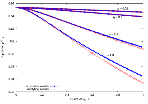
The final analytical expression for the finite-time σ ^ x subscript ^ 𝜎 𝑥 \hat{\sigma}_{x} 45 60 η 𝜂 \eta ρ 11 ( t ) subscript 𝜌 11 𝑡 \rho_{11}\left(t\right) η 𝜂 \eta
Figure 1: (Color online) Comparison between the time evolution of the population
in the eigenbasis of σ ^ x subscript ^ 𝜎 𝑥 \hat{\sigma}_{x} ρ 11 ( x ) ( t ) superscript subscript 𝜌 11 𝑥 𝑡 \rho_{11}^{\left(x\right)}\left(t\right) λ 2 = 4 ω c superscript 𝜆 2 4 subscript 𝜔 𝑐 \lambda^{2}=4\omega_{c} η 𝜂 \eta 1 2 ( | 1 ⟩ + e i π / 4 | 2 ⟩ ) 1 2 ket 1 superscript 𝑒 𝑖 𝜋 4 ket 2 \frac{1}{\sqrt{2}}\left(\left|1\right\rangle+e^{i\pi/4}\left|2\right\rangle\right)
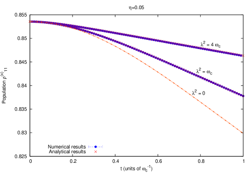
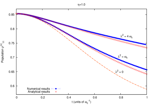
Having confirmed the reliability of our results, we proceed to compare
the noisy measurement described by our formalism with the case where
the system is not being measured. As can be seen in Fig. 2, systems
evolving only under the influence of the environment (λ 2 = 0 superscript 𝜆 2 0 \lambda^{2}=0 λ 2 > 0 superscript 𝜆 2 0 \lambda^{2}>0 σ ^ x subscript ^ 𝜎 𝑥 \hat{\sigma}_{x}
Figure 2: (Color online) Time evolution of the population in the eigenbasis
of σ ^ x subscript ^ 𝜎 𝑥 \hat{\sigma}_{x} λ = 0 𝜆 0 \lambda=0
The meaning of this phenomenon is straightforward: a difference between
the initial value of the population (instant t 0 subscript 𝑡 0 t_{0} t f subscript 𝑡 𝑓 t_{f} ρ 11 ( t 0 ) subscript 𝜌 11 subscript 𝑡 0 \rho_{11}\left(t_{0}\right) ρ 11 ( t f ) subscript 𝜌 11 subscript 𝑡 𝑓 \rho_{11}\left(t_{f}\right) ϵ = | ρ 11 ( t f ) − ρ 11 ( t 0 ) | italic-ϵ subscript 𝜌 11 subscript 𝑡 𝑓 subscript 𝜌 11 subscript 𝑡 0 \epsilon=\left|\rho_{11}\left(t_{f}\right)-\rho_{11}\left(t_{0}\right)\right| t 0 subscript 𝑡 0 t_{0} ϵ italic-ϵ \epsilon
The fact that a finite-time measurement helps to preserve the initial
value of the population of a system also shows that a naïve approach
to a noisy measurement will overestimate the error. Given that a measurement
ends at a time t f subscript 𝑡 𝑓 t_{f} t 0 < t f subscript 𝑡 0 subscript 𝑡 𝑓 t_{0}<t_{f} t f − t 0 subscript 𝑡 𝑓 subscript 𝑡 0 t_{f}-t_{0}
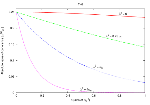
Finally, it is important to notice that this protection against error
depends on whether the observable measured commutes with the interaction
Hamiltonian. In the measurement described above, the observable σ ^ x subscript ^ 𝜎 𝑥 \hat{\sigma}_{x} σ ^ z subscript ^ 𝜎 𝑧 \hat{\sigma}_{z}
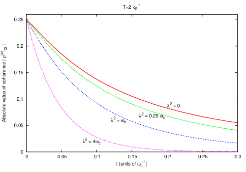
Figure 3: (Color online) Time evolution of the absolute value of the coherence
in the eigenbasis of σ ^ z subscript ^ 𝜎 𝑧 \hat{\sigma}_{z} η = 0.05 𝜂 0.05 \eta=0.05 σ ^ z subscript ^ 𝜎 𝑧 \hat{\sigma}_{z} 31
In short, when the observable measured is σ ^ z subscript ^ 𝜎 𝑧 \hat{\sigma}_{z} σ ^ x subscript ^ 𝜎 𝑥 \hat{\sigma}_{x}
VI Conclusions and Perspectives
In this work, we have analyzed a two-state system subject to finite-time
measurements that commute or anti-commute with the interaction Hamiltonian
which couples the system with a phase-noisy environment. In the first
case, we have shown that the complete analytical results for a finite-time
measurement in any temperature - seen in Eqs. (28 30 31 45 60
Our approach of considering the system interacting with the environment,
but the apparatus interacting only with the system, through our treatment
of the Lindblad equation, is novel. However, we
have treated the problem with a series of simplifications, namely:
zero temperature for the initial state of the environment, Ohmic density
of states, and the neglect of the system Hamiltonian when measuring
an observable that does not commute with it. Subsequent studies may
use our method in more general cases, even varying the number of states
of the system considered. A first step in the direction of studying
systems interacting with environments initially at temperature T > 0 𝑇 0 T>0 43
The present formalism does not allow us to approach the possibility
of the state measured being different from an eigenvalue of the system,
as considered in some works on quantum theory of measurement key-40 key-13 ; key-14 ; key-15 key-47 key-48 key-48
Acknowledgements.
C. A. Brasil acknowledges support from Coordenação de Aperfeiçoamento
de Pessoal de Nível Superior (CAPES), Brazil.
L. A. de Castro acknowledges support from Fundação de Amparo à Pesquisa
do Estado de São Paulo (FAPESP), Brazil, project number 2009/12460-0.
R. d. J. Napolitano acknowledges support from Conselho Nacional de
Desenvolvimento Científico e Tecnológico (CNPq), Brazil.
Appendix A: Calculation of the environment degrees of freedom (Sec.
iii-b)
Using Eq. (15
( I ) 𝐼 \displaystyle\left(I\right) Tr B { e − B ^ ^ t B ^ { e B ^ ^ ( t − t ′ ) [ ( e B ^ ^ t ′ ρ ^ B ) B ^ ] } } subscript Tr 𝐵 superscript 𝑒 ^ ^ 𝐵 𝑡 ^ 𝐵 superscript 𝑒 ^ ^ 𝐵 𝑡 superscript 𝑡 ′ delimited-[] superscript 𝑒 ^ ^ 𝐵 superscript 𝑡 ′ subscript ^ 𝜌 𝐵 ^ 𝐵 \displaystyle\mathrm{Tr}_{B}\left\{e^{-\hat{\hat{B}}t}\hat{B}\left\{e^{\hat{\hat{B}}\left(t-t^{\prime}\right)}\left[\left(e^{\hat{\hat{B}}t^{\prime}}\hat{\rho}_{B}\right)\hat{B}\right]\right\}\right\} = Tr B { e i H ^ B ℏ t B ^ e − i H ^ B ℏ t ρ ^ B e i H ^ B ℏ t ′ B ^ e − i H ^ B ℏ t ′ } , absent subscript Tr 𝐵 superscript 𝑒 𝑖 subscript ^ 𝐻 𝐵 Planck-constant-over-2-pi 𝑡 ^ 𝐵 superscript 𝑒 𝑖 subscript ^ 𝐻 𝐵 Planck-constant-over-2-pi 𝑡 subscript ^ 𝜌 𝐵 superscript 𝑒 𝑖 subscript ^ 𝐻 𝐵 Planck-constant-over-2-pi superscript 𝑡 ′ ^ 𝐵 superscript 𝑒 𝑖 subscript ^ 𝐻 𝐵 Planck-constant-over-2-pi superscript 𝑡 ′ \displaystyle=\mathrm{Tr}_{B}\left\{e^{i\frac{\hat{H}_{B}}{\hbar}t}\hat{B}e^{-i\frac{\hat{H}_{B}}{\hbar}t}\hat{\rho}_{B}e^{i\frac{\hat{H}_{B}}{\hbar}t^{\prime}}\hat{B}e^{-i\frac{\hat{H}_{B}}{\hbar}t^{\prime}}\right\}, (61)
( I I ) 𝐼 𝐼 \displaystyle\left(II\right) Tr B { e − B ^ ^ t { e B ^ ^ ( t − t ′ ) [ ( e B ^ ^ t ′ ρ ^ B ) B ^ ] } B ^ } = subscript Tr 𝐵 superscript 𝑒 ^ ^ 𝐵 𝑡 superscript 𝑒 ^ ^ 𝐵 𝑡 superscript 𝑡 ′ delimited-[] superscript 𝑒 ^ ^ 𝐵 superscript 𝑡 ′ subscript ^ 𝜌 𝐵 ^ 𝐵 ^ 𝐵 absent \displaystyle\mathrm{Tr}_{B}\left\{e^{-\hat{\hat{B}}t}\left\{e^{\hat{\hat{B}}\left(t-t^{\prime}\right)}\left[\left(e^{\hat{\hat{B}}t^{\prime}}\hat{\rho}_{B}\right)\hat{B}\right]\right\}\hat{B}\right\}= Tr B { e i H ^ B ℏ t B ^ e − i H ^ B ℏ t ρ ^ B e i H ^ B ℏ t ′ B ^ e − i H ^ B ℏ t ′ } , subscript Tr 𝐵 superscript 𝑒 𝑖 subscript ^ 𝐻 𝐵 Planck-constant-over-2-pi 𝑡 ^ 𝐵 superscript 𝑒 𝑖 subscript ^ 𝐻 𝐵 Planck-constant-over-2-pi 𝑡 subscript ^ 𝜌 𝐵 superscript 𝑒 𝑖 subscript ^ 𝐻 𝐵 Planck-constant-over-2-pi superscript 𝑡 ′ ^ 𝐵 superscript 𝑒 𝑖 subscript ^ 𝐻 𝐵 Planck-constant-over-2-pi superscript 𝑡 ′ \displaystyle\mathrm{Tr}_{B}\left\{e^{i\frac{\hat{H}_{B}}{\hbar}t}\hat{B}e^{-i\frac{\hat{H}_{B}}{\hbar}t}\hat{\rho}_{B}e^{i\frac{\hat{H}_{B}}{\hbar}t^{\prime}}\hat{B}e^{-i\frac{\hat{H}_{B}}{\hbar}t^{\prime}}\right\}, (62)
( I I I ) 𝐼 𝐼 𝐼 \displaystyle\left(III\right) Tr B { e − B ^ ^ t B ^ { e B ^ ^ ( t − t ′ ) [ B ^ ( e B ^ ^ t ′ ρ ^ B ) ] } } = subscript Tr 𝐵 superscript 𝑒 ^ ^ 𝐵 𝑡 ^ 𝐵 superscript 𝑒 ^ ^ 𝐵 𝑡 superscript 𝑡 ′ delimited-[] ^ 𝐵 superscript 𝑒 ^ ^ 𝐵 superscript 𝑡 ′ subscript ^ 𝜌 𝐵 absent \displaystyle\mathrm{Tr}_{B}\left\{e^{-\hat{\hat{B}}t}\hat{B}\left\{e^{\hat{\hat{B}}\left(t-t^{\prime}\right)}\left[\hat{B}\left(e^{\hat{\hat{B}}t^{\prime}}\hat{\rho}_{B}\right)\right]\right\}\right\}= Tr B { e i H ^ B ℏ t ′ B ^ e − i H ^ B ℏ t ′ ρ ^ B e i H ^ B ℏ t B ^ e − i H ^ B ℏ t } , subscript Tr 𝐵 superscript 𝑒 𝑖 subscript ^ 𝐻 𝐵 Planck-constant-over-2-pi superscript 𝑡 ′ ^ 𝐵 superscript 𝑒 𝑖 subscript ^ 𝐻 𝐵 Planck-constant-over-2-pi superscript 𝑡 ′ subscript ^ 𝜌 𝐵 superscript 𝑒 𝑖 subscript ^ 𝐻 𝐵 Planck-constant-over-2-pi 𝑡 ^ 𝐵 superscript 𝑒 𝑖 subscript ^ 𝐻 𝐵 Planck-constant-over-2-pi 𝑡 \displaystyle\mathrm{Tr}_{B}\left\{e^{i\frac{\hat{H}_{B}}{\hbar}t^{\prime}}\hat{B}e^{-i\frac{\hat{H}_{B}}{\hbar}t^{\prime}}\hat{\rho}_{B}e^{i\frac{\hat{H}_{B}}{\hbar}t}\hat{B}e^{-i\frac{\hat{H}_{B}}{\hbar}t}\right\}, (63)
( I V ) 𝐼 𝑉 \displaystyle\left(IV\right) Tr B { e − B ^ ^ t { e B ^ ^ ( t − t ′ ) [ B ^ ( e B ^ ^ t ′ ρ ^ B ) ] } B ^ } = subscript Tr 𝐵 superscript 𝑒 ^ ^ 𝐵 𝑡 superscript 𝑒 ^ ^ 𝐵 𝑡 superscript 𝑡 ′ delimited-[] ^ 𝐵 superscript 𝑒 ^ ^ 𝐵 superscript 𝑡 ′ subscript ^ 𝜌 𝐵 ^ 𝐵 absent \displaystyle\mathrm{Tr}_{B}\left\{e^{-\hat{\hat{B}}t}\left\{e^{\hat{\hat{B}}\left(t-t^{\prime}\right)}\left[\hat{B}\left(e^{\hat{\hat{B}}t^{\prime}}\hat{\rho}_{B}\right)\right]\right\}\hat{B}\right\}= Tr B { e i H ^ B ℏ t ′ B ^ e − i H ^ B ℏ t ′ ρ ^ B e i H ^ B ℏ t B ^ e − i H ^ B ℏ t } . subscript Tr 𝐵 superscript 𝑒 𝑖 subscript ^ 𝐻 𝐵 Planck-constant-over-2-pi superscript 𝑡 ′ ^ 𝐵 superscript 𝑒 𝑖 subscript ^ 𝐻 𝐵 Planck-constant-over-2-pi superscript 𝑡 ′ subscript ^ 𝜌 𝐵 superscript 𝑒 𝑖 subscript ^ 𝐻 𝐵 Planck-constant-over-2-pi 𝑡 ^ 𝐵 superscript 𝑒 𝑖 subscript ^ 𝐻 𝐵 Planck-constant-over-2-pi 𝑡 \displaystyle\mathrm{Tr}_{B}\left\{e^{i\frac{\hat{H}_{B}}{\hbar}t^{\prime}}\hat{B}e^{-i\frac{\hat{H}_{B}}{\hbar}t^{\prime}}\hat{\rho}_{B}e^{i\frac{\hat{H}_{B}}{\hbar}t}\hat{B}e^{-i\frac{\hat{H}_{B}}{\hbar}t}\right\}. (64)
Let us insert, then, Eqs. (61 62 63 64 17
P ^ ^ G ^ ^ ( t ) G ^ ^ ( t ′ ) P ^ ^ α ^ ( t ) ^ ^ 𝑃 ^ ^ 𝐺 𝑡 ^ ^ 𝐺 superscript 𝑡 ′ ^ ^ 𝑃 ^ 𝛼 𝑡 \displaystyle\hat{\hat{P}}\hat{\hat{G}}\left(t\right)\hat{\hat{G}}\left(t^{\prime}\right)\hat{\hat{P}}\hat{\alpha}\left(t\right) = \displaystyle= { e − S ^ ^ t σ ^ z { e S ^ ^ ( t − t ′ ) [ ( e S ^ ^ t ′ R ^ ( t ) ) σ ^ z ] } \displaystyle\left\{e^{-\hat{\hat{S}}t}\hat{\sigma}_{z}\left\{e^{\hat{\hat{S}}\left(t-t^{\prime}\right)}\left[\left(e^{\hat{\hat{S}}t^{\prime}}\hat{R}\left(t\right)\right)\hat{\sigma}_{z}\right]\right\}\right. (65)
− \displaystyle- e − S ^ ^ t { e S ^ ^ ( t − t ′ ) [ ( e S ^ ^ t ′ R ^ ( t ) ) σ ^ z ] } σ ^ z } \displaystyle\left.e^{-\hat{\hat{S}}t}\left\{e^{\hat{\hat{S}}\left(t-t^{\prime}\right)}\left[\left(e^{\hat{\hat{S}}t^{\prime}}\hat{R}\left(t\right)\right)\hat{\sigma}_{z}\right]\right\}\hat{\sigma}_{z}\right\}
× \displaystyle\times Tr B { e i H ^ B ℏ t B ^ e − i H ^ B ℏ t ρ ^ B e i H ^ B ℏ t ′ B ^ e − i H ^ B ℏ t ′ } ⊗ ρ ^ B tensor-product subscript Tr 𝐵 superscript 𝑒 𝑖 subscript ^ 𝐻 𝐵 Planck-constant-over-2-pi 𝑡 ^ 𝐵 superscript 𝑒 𝑖 subscript ^ 𝐻 𝐵 Planck-constant-over-2-pi 𝑡 subscript ^ 𝜌 𝐵 superscript 𝑒 𝑖 subscript ^ 𝐻 𝐵 Planck-constant-over-2-pi superscript 𝑡 ′ ^ 𝐵 superscript 𝑒 𝑖 subscript ^ 𝐻 𝐵 Planck-constant-over-2-pi superscript 𝑡 ′ subscript ^ 𝜌 𝐵 \displaystyle\mathrm{Tr}_{B}\left\{e^{i\frac{\hat{H}_{B}}{\hbar}t}\hat{B}e^{-i\frac{\hat{H}_{B}}{\hbar}t}\hat{\rho}_{B}e^{i\frac{\hat{H}_{B}}{\hbar}t^{\prime}}\hat{B}e^{-i\frac{\hat{H}_{B}}{\hbar}t^{\prime}}\right\}\otimes\hat{\rho}_{B}
+ \displaystyle+ { e − S ^ ^ t { e S ^ ^ ( t − t ′ ) [ σ ^ z ( e S ^ ^ t ′ R ^ ( t ) ) ] } σ ^ z \displaystyle\left\{e^{-\hat{\hat{S}}t}\left\{e^{\hat{\hat{S}}\left(t-t^{\prime}\right)}\left[\hat{\sigma}_{z}\left(e^{\hat{\hat{S}}t^{\prime}}\hat{R}\left(t\right)\right)\right]\right\}\hat{\sigma}_{z}\right.
− \displaystyle- e − S ^ ^ t σ ^ z { e S ^ ^ ( t − t ′ ) [ σ ^ z ( e S ^ ^ t ′ R ^ ( t ) ) ] } } \displaystyle\left.e^{-\hat{\hat{S}}t}\hat{\sigma}_{z}\left\{e^{\hat{\hat{S}}\left(t-t^{\prime}\right)}\left[\hat{\sigma}_{z}\left(e^{\hat{\hat{S}}t^{\prime}}\hat{R}\left(t\right)\right)\right]\right\}\right\}
× \displaystyle\times Tr B { e i H ^ B ℏ t ′ B ^ e − i H ^ B ℏ t ′ ρ ^ B e i H ^ B ℏ t B ^ e − i H ^ B ℏ t } ⊗ ρ ^ B . tensor-product subscript Tr 𝐵 superscript 𝑒 𝑖 subscript ^ 𝐻 𝐵 Planck-constant-over-2-pi superscript 𝑡 ′ ^ 𝐵 superscript 𝑒 𝑖 subscript ^ 𝐻 𝐵 Planck-constant-over-2-pi superscript 𝑡 ′ subscript ^ 𝜌 𝐵 superscript 𝑒 𝑖 subscript ^ 𝐻 𝐵 Planck-constant-over-2-pi 𝑡 ^ 𝐵 superscript 𝑒 𝑖 subscript ^ 𝐻 𝐵 Planck-constant-over-2-pi 𝑡 subscript ^ 𝜌 𝐵 \displaystyle\mathrm{Tr}_{B}\left\{e^{i\frac{\hat{H}_{B}}{\hbar}t^{\prime}}\hat{B}e^{-i\frac{\hat{H}_{B}}{\hbar}t^{\prime}}\hat{\rho}_{B}e^{i\frac{\hat{H}_{B}}{\hbar}t}\hat{B}e^{-i\frac{\hat{H}_{B}}{\hbar}t}\right\}\otimes\hat{\rho}_{B}.
The two terms in Eq. (65
{ t → t ′ t ′ → t cases 𝑡 → absent superscript 𝑡 ′ superscript 𝑡 ′ → absent 𝑡 \begin{cases}t&\rightarrow t^{\prime}\\
t^{\prime}&\rightarrow t\end{cases}
to obtain the second. To take the partial trace, we use the Fock-state
basis | n 1 ⟩ ⊗ | n 2 ⟩ … ≡ ∏ 𝑚 | n m ⟩ tensor-product ket subscript 𝑛 1 ket subscript 𝑛 2 … 𝑚 product ket subscript 𝑛 𝑚 \left|n_{1}\right\rangle\otimes\left|n_{2}\right\rangle...\equiv\underset{m}{\prod}\left|n_{m}\right\rangle
Tr B { } → ∑ n 1 , n 2 , … [ ∏ 𝑚 ⟨ n m | ] [ ∏ 𝑚 | n m ⟩ ] → subscript Tr 𝐵
subscript 𝑛 1 subscript 𝑛 2 …
delimited-[] 𝑚 product bra subscript 𝑛 𝑚 delimited-[] 𝑚 product ket subscript 𝑛 𝑚 \mathrm{Tr}_{B}\left\{\right\}\rightarrow\underset{n_{1},n_{2},...}{\sum}\left[\underset{m}{\prod}\left\langle n_{m}\right|\right]\left[\underset{m}{\prod}\left|n_{m}\right\rangle\right]
and we obtain key-42
e i t ∑ 𝑙 ω l b ^ l † b ^ l ∑ 𝑘 ( g k ∗ b ^ k + g k b ^ k † ) e − i t ∑ 𝑙 ω l b ^ l † b ^ l = ∑ 𝑘 ( g k ∗ b ^ k e − i ω k t + g k b ^ k † e i ω k t ) . superscript 𝑒 𝑖 𝑡 𝑙 subscript 𝜔 𝑙 superscript subscript ^ 𝑏 𝑙 † subscript ^ 𝑏 𝑙 𝑘 superscript subscript 𝑔 𝑘 subscript ^ 𝑏 𝑘 subscript 𝑔 𝑘 superscript subscript ^ 𝑏 𝑘 † superscript 𝑒 𝑖 𝑡 𝑙 subscript 𝜔 𝑙 superscript subscript ^ 𝑏 𝑙 † subscript ^ 𝑏 𝑙 𝑘 superscript subscript 𝑔 𝑘 subscript ^ 𝑏 𝑘 superscript 𝑒 𝑖 subscript 𝜔 𝑘 𝑡 subscript 𝑔 𝑘 superscript subscript ^ 𝑏 𝑘 † superscript 𝑒 𝑖 subscript 𝜔 𝑘 𝑡 e^{it\underset{l}{\sum}\omega_{l}\hat{b}_{l}^{\dagger}\hat{b}_{l}}\underset{k}{\sum}\left(g_{k}^{*}\hat{b}_{k}+g_{k}\hat{b}_{k}^{\dagger}\right)e^{-it\underset{l}{\sum}\omega_{l}\hat{b}_{l}^{\dagger}\hat{b}_{l}}=\underset{k}{\sum}\left(g_{k}^{*}\hat{b}_{k}e^{-i\omega_{k}t}+g_{k}\hat{b}_{k}^{\dagger}e^{i\omega_{k}t}\right). (66)
if we specify H ^ B subscript ^ 𝐻 𝐵 \hat{H}_{B} B ^ ^ 𝐵 \hat{B} 9 10 66
Tr B { e i H ^ B ℏ t B ^ e − i H ^ B ℏ t ρ ^ B e i H ^ B ℏ t ′ B ^ e − i H ^ B ℏ t ′ } subscript Tr 𝐵 superscript 𝑒 𝑖 subscript ^ 𝐻 𝐵 Planck-constant-over-2-pi 𝑡 ^ 𝐵 superscript 𝑒 𝑖 subscript ^ 𝐻 𝐵 Planck-constant-over-2-pi 𝑡 subscript ^ 𝜌 𝐵 superscript 𝑒 𝑖 subscript ^ 𝐻 𝐵 Planck-constant-over-2-pi superscript 𝑡 ′ ^ 𝐵 superscript 𝑒 𝑖 subscript ^ 𝐻 𝐵 Planck-constant-over-2-pi superscript 𝑡 ′ \displaystyle\mathrm{Tr}_{B}\left\{e^{i\frac{\hat{H}_{B}}{\hbar}t}\hat{B}e^{-i\frac{\hat{H}_{B}}{\hbar}t}\hat{\rho}_{B}e^{i\frac{\hat{H}_{B}}{\hbar}t^{\prime}}\hat{B}e^{-i\frac{\hat{H}_{B}}{\hbar}t^{\prime}}\right\} = \displaystyle= ∑ n 1 , n 2 , … [ ∏ 𝑚 ⟨ n m | ] ∑ 𝑙 ( g l ∗ b ^ l e − i ω l t + g l b ^ l † e i ω l t ) subscript 𝑛 1 subscript 𝑛 2 …
delimited-[] 𝑚 product bra subscript 𝑛 𝑚 𝑙 superscript subscript 𝑔 𝑙 subscript ^ 𝑏 𝑙 superscript 𝑒 𝑖 subscript 𝜔 𝑙 𝑡 subscript 𝑔 𝑙 superscript subscript ^ 𝑏 𝑙 † superscript 𝑒 𝑖 subscript 𝜔 𝑙 𝑡 \displaystyle\underset{n_{1},n_{2},...}{\sum}\left[\underset{m}{\prod}\left\langle n_{m}\right|\right]\underset{l}{\sum}\left(g_{l}^{*}\hat{b}_{l}e^{-i\omega_{l}t}+g_{l}\hat{b}_{l}^{\dagger}e^{i\omega_{l}t}\right)
× \displaystyle\times ρ ^ B ∑ 𝑘 ( g k ∗ b ^ k e − i ω k t ′ + g k b ^ k † e i ω k t ′ ) [ ∏ 𝑚 | n m ⟩ ] . subscript ^ 𝜌 𝐵 𝑘 superscript subscript 𝑔 𝑘 subscript ^ 𝑏 𝑘 superscript 𝑒 𝑖 subscript 𝜔 𝑘 superscript 𝑡 ′ subscript 𝑔 𝑘 superscript subscript ^ 𝑏 𝑘 † superscript 𝑒 𝑖 subscript 𝜔 𝑘 superscript 𝑡 ′ delimited-[] 𝑚 product ket subscript 𝑛 𝑚 \displaystyle\hat{\rho}_{B}\underset{k}{\sum}\left(g_{k}^{*}\hat{b}_{k}e^{-i\omega_{k}t^{\prime}}+g_{k}\hat{b}_{k}^{\dagger}e^{i\omega_{k}t^{\prime}}\right)\left[\underset{m}{\prod}\left|n_{m}\right\rangle\right].
With (11
Tr B { e i H ^ B ℏ t B ^ e − i H ^ B ℏ t ρ ^ B e i H ^ B ℏ t ′ B ^ e − i H ^ B ℏ t ′ } subscript Tr 𝐵 superscript 𝑒 𝑖 subscript ^ 𝐻 𝐵 Planck-constant-over-2-pi 𝑡 ^ 𝐵 superscript 𝑒 𝑖 subscript ^ 𝐻 𝐵 Planck-constant-over-2-pi 𝑡 subscript ^ 𝜌 𝐵 superscript 𝑒 𝑖 subscript ^ 𝐻 𝐵 Planck-constant-over-2-pi superscript 𝑡 ′ ^ 𝐵 superscript 𝑒 𝑖 subscript ^ 𝐻 𝐵 Planck-constant-over-2-pi superscript 𝑡 ′ \displaystyle\mathrm{Tr}_{B}\left\{e^{i\frac{\hat{H}_{B}}{\hbar}t}\hat{B}e^{-i\frac{\hat{H}_{B}}{\hbar}t}\hat{\rho}_{B}e^{i\frac{\hat{H}_{B}}{\hbar}t^{\prime}}\hat{B}e^{-i\frac{\hat{H}_{B}}{\hbar}t^{\prime}}\right\} = \displaystyle= ∑ 𝑙 | g l | 2 [ e i ω l ( t − t ′ ) + e i ω l ( t − t ′ ) e ℏ β ω l − 1 + e − i ω l ( t − t ′ ) e ℏ β ω l − 1 ] 𝑙 superscript subscript 𝑔 𝑙 2 delimited-[] superscript 𝑒 𝑖 subscript 𝜔 𝑙 𝑡 superscript 𝑡 ′ superscript 𝑒 𝑖 subscript 𝜔 𝑙 𝑡 superscript 𝑡 ′ superscript 𝑒 Planck-constant-over-2-pi 𝛽 subscript 𝜔 𝑙 1 superscript 𝑒 𝑖 subscript 𝜔 𝑙 𝑡 superscript 𝑡 ′ superscript 𝑒 Planck-constant-over-2-pi 𝛽 subscript 𝜔 𝑙 1 \displaystyle\underset{l}{\sum}\left|g_{l}\right|^{2}\left[e^{i\omega_{l}\left(t-t^{\prime}\right)}+\frac{e^{i\omega_{l}\left(t-t^{\prime}\right)}}{e^{\hbar\beta\omega_{l}}-1}+\frac{e^{-i\omega_{l}\left(t-t^{\prime}\right)}}{e^{\hbar\beta\omega_{l}}-1}\right]
= \displaystyle= ∑ 𝑙 | g l | 2 [ e i ω l ( t − t ′ ) + 2 cos [ ω l ( t − t ′ ) ] e ℏ β ω l − 1 ] , 𝑙 superscript subscript 𝑔 𝑙 2 delimited-[] superscript 𝑒 𝑖 subscript 𝜔 𝑙 𝑡 superscript 𝑡 ′ 2 subscript 𝜔 𝑙 𝑡 superscript 𝑡 ′ superscript 𝑒 Planck-constant-over-2-pi 𝛽 subscript 𝜔 𝑙 1 \displaystyle\underset{l}{\sum}\left|g_{l}\right|^{2}\left[e^{i\omega_{l}\left(t-t^{\prime}\right)}+\frac{2\cos\left[\omega_{l}\left(t-t^{\prime}\right)\right]}{e^{\hbar\beta\omega_{l}}-1}\right],
or, more simply,
Tr B { e i H ^ B ℏ t B ^ e − i H ^ B ℏ t ρ ^ B e i H ^ B ℏ t ′ B ^ e − i H ^ B ℏ t ′ } subscript Tr 𝐵 superscript 𝑒 𝑖 subscript ^ 𝐻 𝐵 Planck-constant-over-2-pi 𝑡 ^ 𝐵 superscript 𝑒 𝑖 subscript ^ 𝐻 𝐵 Planck-constant-over-2-pi 𝑡 subscript ^ 𝜌 𝐵 superscript 𝑒 𝑖 subscript ^ 𝐻 𝐵 Planck-constant-over-2-pi superscript 𝑡 ′ ^ 𝐵 superscript 𝑒 𝑖 subscript ^ 𝐻 𝐵 Planck-constant-over-2-pi superscript 𝑡 ′ \displaystyle\mathrm{Tr}_{B}\left\{e^{i\frac{\hat{H}_{B}}{\hbar}t}\hat{B}e^{-i\frac{\hat{H}_{B}}{\hbar}t}\hat{\rho}_{B}e^{i\frac{\hat{H}_{B}}{\hbar}t^{\prime}}\hat{B}e^{-i\frac{\hat{H}_{B}}{\hbar}t^{\prime}}\right\} = \displaystyle= ∑ 𝑙 | g l | 2 { coth ( ℏ β ω l 2 ) cos [ ω l ( t − t ′ ) ] \displaystyle\underset{l}{\sum}\left|g_{l}\right|^{2}\left\{\coth\left(\frac{\hbar\beta\omega_{l}}{2}\right)\cos\left[\omega_{l}\left(t-t^{\prime}\right)\right]\right. (67)
+ \displaystyle+ i sin [ ω l ( t − t ′ ) ] } . \displaystyle\left.i\sin\left[\omega_{l}\left(t-t^{\prime}\right)\right]\right\}.
As explained above, the change of varibles
{ t → t ′ t ′ → t cases 𝑡 → absent superscript 𝑡 ′ superscript 𝑡 ′ → absent 𝑡 \begin{cases}t&\rightarrow t^{\prime}\\
t^{\prime}&\rightarrow t\end{cases}
in Eq. (67 65
Tr B { e i H ^ B ℏ t ′ B ^ e − i H ^ B ℏ t ′ ρ ^ B e i H ^ B ℏ t B ^ e − i H ^ B ℏ t } subscript Tr 𝐵 superscript 𝑒 𝑖 subscript ^ 𝐻 𝐵 Planck-constant-over-2-pi superscript 𝑡 ′ ^ 𝐵 superscript 𝑒 𝑖 subscript ^ 𝐻 𝐵 Planck-constant-over-2-pi superscript 𝑡 ′ subscript ^ 𝜌 𝐵 superscript 𝑒 𝑖 subscript ^ 𝐻 𝐵 Planck-constant-over-2-pi 𝑡 ^ 𝐵 superscript 𝑒 𝑖 subscript ^ 𝐻 𝐵 Planck-constant-over-2-pi 𝑡 \displaystyle\mathrm{Tr}_{B}\left\{e^{i\frac{\hat{H}_{B}}{\hbar}t^{\prime}}\hat{B}e^{-i\frac{\hat{H}_{B}}{\hbar}t^{\prime}}\hat{\rho}_{B}e^{i\frac{\hat{H}_{B}}{\hbar}t}\hat{B}e^{-i\frac{\hat{H}_{B}}{\hbar}t}\right\} = \displaystyle= ∑ 𝑙 | g l | 2 { coth ( ℏ β ω l 2 ) cos [ ω l ( t − t ′ ) ] \displaystyle\underset{l}{\sum}\left|g_{l}\right|^{2}\left\{\coth\left(\frac{\hbar\beta\omega_{l}}{2}\right)\cos\left[\omega_{l}\left(t-t^{\prime}\right)\right]\right. (68)
− \displaystyle- i sin [ ω l ( t − t ′ ) ] } . \displaystyle\left.i\sin\left[\omega_{l}\left(t-t^{\prime}\right)\right]\right\}.
The final result, Eq. (18 67 68 65
Appendix E: the differential equations for the case of L ^ ( S ) = λ σ ^ x superscript ^ 𝐿 𝑆 𝜆 subscript ^ 𝜎 𝑥 \hat{L}^{\left(S\right)}=\lambda\hat{\sigma}_{x}
Using the definitions (33 34 35
e S ^ ^ t ′ R ^ ( t ) superscript 𝑒 ^ ^ 𝑆 superscript 𝑡 ′ ^ 𝑅 𝑡 \displaystyle e^{\hat{\hat{S}}t^{\prime}}\hat{R}\left(t\right) = \displaystyle= e S ^ ^ t ′ ( r 11 r 12 r 21 r 22 ) = ( r 11 ( 0 ) r 12 ( 0 ) r 21 ( 0 ) r 22 ( 0 ) ) , superscript 𝑒 ^ ^ 𝑆 superscript 𝑡 ′ subscript 𝑟 11 subscript 𝑟 12 subscript 𝑟 21 subscript 𝑟 22 superscript subscript 𝑟 11 0 superscript subscript 𝑟 12 0 superscript subscript 𝑟 21 0 superscript subscript 𝑟 22 0 \displaystyle e^{\hat{\hat{S}}t^{\prime}}\left(\begin{array}[]{cc}r_{11}&r_{12}\\
r_{21}&r_{22}\end{array}\right)=\left(\begin{array}[]{cc}r_{11}^{\left(0\right)}&r_{12}^{\left(0\right)}\\
r_{21}^{\left(0\right)}&r_{22}^{\left(0\right)}\end{array}\right),
where
{ r 11 ( 0 ) = r 11 − r 22 2 e − 2 λ 2 t ′ + r 11 + r 22 2 , r 22 ( 0 ) = − r 11 − r 22 2 e − 2 λ 2 t ′ + r 11 + r 22 2 , cases superscript subscript 𝑟 11 0 absent subscript 𝑟 11 subscript 𝑟 22 2 superscript 𝑒 2 superscript 𝜆 2 superscript 𝑡 ′ subscript 𝑟 11 subscript 𝑟 22 2 superscript subscript 𝑟 22 0 absent subscript 𝑟 11 subscript 𝑟 22 2 superscript 𝑒 2 superscript 𝜆 2 superscript 𝑡 ′ subscript 𝑟 11 subscript 𝑟 22 2 \begin{cases}r_{11}^{\left(0\right)}=&\frac{r_{11}-r_{22}}{2}e^{-2\lambda^{2}t^{\prime}}+\frac{r_{11}+r_{22}}{2},\\
r_{22}^{\left(0\right)}=&-\frac{r_{11}-r_{22}}{2}e^{-2\lambda^{2}t^{\prime}}+\frac{r_{11}+r_{22}}{2},\end{cases} (86)
and
{ r 12 ( 0 ) = e − λ 2 t ′ Ω [ Ω cosh ( Ω t ′ ) r 12 − i 2 ω 0 sinh ( Ω t ′ ) r 12 + λ 2 sinh ( Ω t ′ ) r 21 ] , r 21 ( 0 ) = e − λ 2 t ′ Ω [ Ω cosh ( Ω t ′ ) r 21 + i 2 ω 0 sinh ( Ω t ′ ) r 21 + λ 2 sinh ( Ω t ′ ) r 12 ] . cases superscript subscript 𝑟 12 0 absent superscript 𝑒 superscript 𝜆 2 superscript 𝑡 ′ Ω delimited-[] Ω Ω superscript 𝑡 ′ subscript 𝑟 12 𝑖 2 subscript 𝜔 0 Ω superscript 𝑡 ′ subscript 𝑟 12 superscript 𝜆 2 Ω superscript 𝑡 ′ subscript 𝑟 21 superscript subscript 𝑟 21 0 absent superscript 𝑒 superscript 𝜆 2 superscript 𝑡 ′ Ω delimited-[] Ω Ω superscript 𝑡 ′ subscript 𝑟 21 𝑖 2 subscript 𝜔 0 Ω superscript 𝑡 ′ subscript 𝑟 21 superscript 𝜆 2 Ω superscript 𝑡 ′ subscript 𝑟 12 \begin{cases}r_{12}^{\left(0\right)}=&\frac{e^{-\lambda^{2}t^{\prime}}}{\Omega}\left[\Omega\cosh\left(\Omega t^{\prime}\right)r_{12}-i2\omega_{0}\sinh\left(\Omega t^{\prime}\right)r_{12}+\lambda^{2}\sinh\left(\Omega t^{\prime}\right)r_{21}\right],\\
r_{21}^{\left(0\right)}=&\frac{e^{-\lambda^{2}t^{\prime}}}{\Omega}\left[\Omega\cosh\left(\Omega t^{\prime}\right)r_{21}+i2\omega_{0}\sinh\left(\Omega t^{\prime}\right)r_{21}+\lambda^{2}\sinh\left(\Omega t^{\prime}\right)r_{12}\right].\end{cases} (87)
Now we can evaluate the terms between brackets on (20
e S ^ ^ ( t − t ′ ) [ σ ^ z ( e S ^ ^ t ′ R ^ ( t ) ) ] superscript 𝑒 ^ ^ 𝑆 𝑡 superscript 𝑡 ′ delimited-[] subscript ^ 𝜎 𝑧 superscript 𝑒 ^ ^ 𝑆 superscript 𝑡 ′ ^ 𝑅 𝑡 \displaystyle e^{\hat{\hat{S}}\left(t-t^{\prime}\right)}\left[\hat{\sigma}_{z}\left(e^{\hat{\hat{S}}t^{\prime}}\hat{R}\left(t\right)\right)\right] = \displaystyle= ( r 11 ( 1 ) r 12 ( 1 ) r 21 ( 1 ) r 22 ( 1 ) ) superscript subscript 𝑟 11 1 superscript subscript 𝑟 12 1 superscript subscript 𝑟 21 1 superscript subscript 𝑟 22 1 \displaystyle\left(\begin{array}[]{cc}r_{11}^{\left(1\right)}&r_{12}^{\left(1\right)}\\
r_{21}^{\left(1\right)}&r_{22}^{\left(1\right)}\end{array}\right)
and
e S ^ ^ ( t − t ′ ) [ ( e S ^ ^ t ′ R ^ ( t ) ) σ ^ z ] superscript 𝑒 ^ ^ 𝑆 𝑡 superscript 𝑡 ′ delimited-[] superscript 𝑒 ^ ^ 𝑆 superscript 𝑡 ′ ^ 𝑅 𝑡 subscript ^ 𝜎 𝑧 \displaystyle e^{\hat{\hat{S}}\left(t-t^{\prime}\right)}\left[\left(e^{\hat{\hat{S}}t^{\prime}}\hat{R}\left(t\right)\right)\hat{\sigma}_{z}\right] = \displaystyle= ( r 11 ( 2 ) r 12 ( 2 ) r 21 ( 2 ) r 22 ( 2 ) ) superscript subscript 𝑟 11 2 superscript subscript 𝑟 12 2 superscript subscript 𝑟 21 2 superscript subscript 𝑟 22 2 \displaystyle\left(\begin{array}[]{cc}r_{11}^{\left(2\right)}&r_{12}^{\left(2\right)}\\
r_{21}^{\left(2\right)}&r_{22}^{\left(2\right)}\end{array}\right)
where, using (86 87
{ r 11 ( 1 ) = r 11 ( 0 ) + r 22 ( 0 ) 2 e − 2 λ 2 ( t − t ′ ) + r 11 ( 0 ) − r 22 ( 0 ) 2 , r 22 ( 1 ) = − r 11 ( 0 ) + r 22 ( 0 ) 2 e − 2 λ 2 ( t − t ′ ) + r 11 ( 0 ) − r 22 ( 0 ) 2 , cases superscript subscript 𝑟 11 1 absent superscript subscript 𝑟 11 0 superscript subscript 𝑟 22 0 2 superscript 𝑒 2 superscript 𝜆 2 𝑡 superscript 𝑡 ′ superscript subscript 𝑟 11 0 superscript subscript 𝑟 22 0 2 superscript subscript 𝑟 22 1 absent superscript subscript 𝑟 11 0 superscript subscript 𝑟 22 0 2 superscript 𝑒 2 superscript 𝜆 2 𝑡 superscript 𝑡 ′ superscript subscript 𝑟 11 0 superscript subscript 𝑟 22 0 2 \displaystyle\begin{cases}r_{11}^{\left(1\right)}=&\frac{r_{11}^{\left(0\right)}+r_{22}^{\left(0\right)}}{2}e^{-2\lambda^{2}\left(t-t^{\prime}\right)}+\frac{r_{11}^{\left(0\right)}-r_{22}^{\left(0\right)}}{2},\\
r_{22}^{\left(1\right)}=&-\frac{r_{11}^{\left(0\right)}+r_{22}^{\left(0\right)}}{2}e^{-2\lambda^{2}\left(t-t^{\prime}\right)}+\frac{r_{11}^{\left(0\right)}-r_{22}^{\left(0\right)}}{2},\end{cases}
{ r 12 ( 1 ) = e − λ 2 ( t − t ′ ) Ω { Ω cosh [ Ω ( t − t ′ ) ] r 12 ( 0 ) − i 2 ω 0 sinh [ Ω ( t − t ′ ) ] r 12 ( 0 ) − λ 2 sinh [ Ω ( t − t ′ ) ] r 21 ( 0 ) } , r 21 ( 1 ) = − e − λ 2 ( t − t ′ ) Ω { Ω cosh [ Ω ( t − t ′ ) ] r 21 ( 0 ) + i 2 ω 0 sinh [ Ω ( t − t ′ ) ] r 21 ( 0 ) − λ 2 sinh [ Ω ( t − t ′ ) ] r 12 ( 0 ) } , cases superscript subscript 𝑟 12 1 absent superscript 𝑒 superscript 𝜆 2 𝑡 superscript 𝑡 ′ Ω Ω Ω 𝑡 superscript 𝑡 ′ superscript subscript 𝑟 12 0 𝑖 2 subscript 𝜔 0 Ω 𝑡 superscript 𝑡 ′ superscript subscript 𝑟 12 0 superscript 𝜆 2 Ω 𝑡 superscript 𝑡 ′ superscript subscript 𝑟 21 0 superscript subscript 𝑟 21 1 absent superscript 𝑒 superscript 𝜆 2 𝑡 superscript 𝑡 ′ Ω Ω Ω 𝑡 superscript 𝑡 ′ superscript subscript 𝑟 21 0 𝑖 2 subscript 𝜔 0 Ω 𝑡 superscript 𝑡 ′ superscript subscript 𝑟 21 0 superscript 𝜆 2 Ω 𝑡 superscript 𝑡 ′ superscript subscript 𝑟 12 0 \displaystyle\begin{cases}r_{12}^{\left(1\right)}=&\frac{e^{-\lambda^{2}\left(t-t^{\prime}\right)}}{\Omega}\left\{\Omega\cosh\left[\Omega\left(t-t^{\prime}\right)\right]r_{12}^{\left(0\right)}-i2\omega_{0}\sinh\left[\Omega\left(t-t^{\prime}\right)\right]r_{12}^{\left(0\right)}-\lambda^{2}\sinh\left[\Omega\left(t-t^{\prime}\right)\right]r_{21}^{\left(0\right)}\right\},\\
r_{21}^{\left(1\right)}=&-\frac{e^{-\lambda^{2}\left(t-t^{\prime}\right)}}{\Omega}\left\{\Omega\cosh\left[\Omega\left(t-t^{\prime}\right)\right]r_{21}^{\left(0\right)}+i2\omega_{0}\sinh\left[\Omega\left(t-t^{\prime}\right)\right]r_{21}^{\left(0\right)}-\lambda^{2}\sinh\left[\Omega\left(t-t^{\prime}\right)\right]r_{12}^{\left(0\right)}\right\},\end{cases}
{ r 11 ( 2 ) = r 11 ( 0 ) + r 22 ( 0 ) 2 e − 2 λ 2 ( t − t ′ ) + r 11 ( 0 ) − r 22 ( 0 ) 2 , r 22 ( 2 ) = − r 11 ( 0 ) + r 22 ( 0 ) 2 e − 2 λ 2 ( t − t ′ ) + r 11 ( 0 ) − r 22 ( 0 ) 2 , cases superscript subscript 𝑟 11 2 absent superscript subscript 𝑟 11 0 superscript subscript 𝑟 22 0 2 superscript 𝑒 2 superscript 𝜆 2 𝑡 superscript 𝑡 ′ superscript subscript 𝑟 11 0 superscript subscript 𝑟 22 0 2 superscript subscript 𝑟 22 2 absent superscript subscript 𝑟 11 0 superscript subscript 𝑟 22 0 2 superscript 𝑒 2 superscript 𝜆 2 𝑡 superscript 𝑡 ′ superscript subscript 𝑟 11 0 superscript subscript 𝑟 22 0 2 \displaystyle\begin{cases}r_{11}^{\left(2\right)}=&\frac{r_{11}^{\left(0\right)}+r_{22}^{\left(0\right)}}{2}e^{-2\lambda^{2}\left(t-t^{\prime}\right)}+\frac{r_{11}^{\left(0\right)}-r_{22}^{\left(0\right)}}{2},\\
r_{22}^{\left(2\right)}=&-\frac{r_{11}^{\left(0\right)}+r_{22}^{\left(0\right)}}{2}e^{-2\lambda^{2}\left(t-t^{\prime}\right)}+\frac{r_{11}^{\left(0\right)}-r_{22}^{\left(0\right)}}{2},\end{cases}
and
{ r 12 ( 2 ) = − e − λ 2 ( t − t ′ ) Ω { Ω cosh [ Ω ( t − t ′ ) ] r 12 ( 0 ) − i 2 ω 0 sinh [ Ω ( t − t ′ ) ] r 12 ( 0 ) − λ 2 sinh [ Ω ( t − t ′ ) ] r 21 ( 0 ) } , r 21 ( 2 ) = e − λ 2 ( t − t ′ ) Ω { Ω cosh [ Ω ( t − t ′ ) ] r 21 ( 0 ) + i 2 ω 0 sinh [ Ω ( t − t ′ ) ] r 21 ( 0 ) − λ 2 sinh [ Ω ( t − t ′ ) ] r 12 ( 0 ) } , cases superscript subscript 𝑟 12 2 absent superscript 𝑒 superscript 𝜆 2 𝑡 superscript 𝑡 ′ Ω Ω Ω 𝑡 superscript 𝑡 ′ superscript subscript 𝑟 12 0 𝑖 2 subscript 𝜔 0 Ω 𝑡 superscript 𝑡 ′ superscript subscript 𝑟 12 0 superscript 𝜆 2 Ω 𝑡 superscript 𝑡 ′ superscript subscript 𝑟 21 0 superscript subscript 𝑟 21 2 absent superscript 𝑒 superscript 𝜆 2 𝑡 superscript 𝑡 ′ Ω Ω Ω 𝑡 superscript 𝑡 ′ superscript subscript 𝑟 21 0 𝑖 2 subscript 𝜔 0 Ω 𝑡 superscript 𝑡 ′ superscript subscript 𝑟 21 0 superscript 𝜆 2 Ω 𝑡 superscript 𝑡 ′ superscript subscript 𝑟 12 0 \displaystyle\begin{cases}r_{12}^{\left(2\right)}=&-\frac{e^{-\lambda^{2}\left(t-t^{\prime}\right)}}{\Omega}\left\{\Omega\cosh\left[\Omega\left(t-t^{\prime}\right)\right]r_{12}^{\left(0\right)}-i2\omega_{0}\sinh\left[\Omega\left(t-t^{\prime}\right)\right]r_{12}^{\left(0\right)}-\lambda^{2}\sinh\left[\Omega\left(t-t^{\prime}\right)\right]r_{21}^{\left(0\right)}\right\},\\
r_{21}^{\left(2\right)}=&\frac{e^{-\lambda^{2}\left(t-t^{\prime}\right)}}{\Omega}\left\{\Omega\cosh\left[\Omega\left(t-t^{\prime}\right)\right]r_{21}^{\left(0\right)}+i2\omega_{0}\sinh\left[\Omega\left(t-t^{\prime}\right)\right]r_{21}^{\left(0\right)}-\lambda^{2}\sinh\left[\Omega\left(t-t^{\prime}\right)\right]r_{12}^{\left(0\right)}\right\},\end{cases}
i.e., { r 11 ( 1 ) = r 11 ( 2 ) r 22 ( 1 ) = r 22 ( 2 ) cases superscript subscript 𝑟 11 1 absent superscript subscript 𝑟 11 2 superscript subscript 𝑟 22 1 absent superscript subscript 𝑟 22 2 \begin{cases}r_{11}^{\left(1\right)}&=r_{11}^{\left(2\right)}\\
r_{22}^{\left(1\right)}&=r_{22}^{\left(2\right)}\end{cases} { r 12 ( 1 ) = − r 12 ( 2 ) r 21 ( 1 ) = − r 21 ( 2 ) cases superscript subscript 𝑟 12 1 absent superscript subscript 𝑟 12 2 superscript subscript 𝑟 21 1 absent superscript subscript 𝑟 21 2 \begin{cases}r_{12}^{\left(1\right)}&=-r_{12}^{\left(2\right)}\\
r_{21}^{\left(1\right)}&=-r_{21}^{\left(2\right)}\end{cases}
The progressive calculus of ( A ) 𝐴 \left(A\right) ( B ) 𝐵 \left(B\right) ( C ) 𝐶 \left(C\right) ( D ) 𝐷 \left(D\right)
( A ) 𝐴 \displaystyle\left(A\right) e − S ^ ^ t σ ^ z { e S ^ ^ ( t − t ′ ) [ ( e S ^ ^ t ′ R ^ ( t ) ) σ ^ z ] } = ( r 11 ( 3 ) r 12 ( 3 ) r 21 ( 3 ) r 22 ( 3 ) ) superscript 𝑒 ^ ^ 𝑆 𝑡 subscript ^ 𝜎 𝑧 superscript 𝑒 ^ ^ 𝑆 𝑡 superscript 𝑡 ′ delimited-[] superscript 𝑒 ^ ^ 𝑆 superscript 𝑡 ′ ^ 𝑅 𝑡 subscript ^ 𝜎 𝑧 superscript subscript 𝑟 11 3 superscript subscript 𝑟 12 3 superscript subscript 𝑟 21 3 superscript subscript 𝑟 22 3 \displaystyle e^{-\hat{\hat{S}}t}\hat{\sigma}_{z}\left\{e^{\hat{\hat{S}}\left(t-t^{\prime}\right)}\left[\left(e^{\hat{\hat{S}}t^{\prime}}\hat{R}\left(t\right)\right)\hat{\sigma}_{z}\right]\right\}=\left(\begin{array}[]{cc}r_{11}^{\left(3\right)}&r_{12}^{\left(3\right)}\\
r_{21}^{\left(3\right)}&r_{22}^{\left(3\right)}\end{array}\right) (92)
with
{ r 11 ( 3 ) = r 11 ( 2 ) + r 22 ( 2 ) 2 e 2 λ 2 t + r 11 ( 2 ) − r 22 ( 2 ) 2 , r 22 ( 3 ) = − r 11 ( 2 ) + r 22 ( 2 ) 2 e 2 λ 2 t + r 11 ( 2 ) − r 22 ( 2 ) 2 , cases superscript subscript 𝑟 11 3 absent superscript subscript 𝑟 11 2 superscript subscript 𝑟 22 2 2 superscript 𝑒 2 superscript 𝜆 2 𝑡 superscript subscript 𝑟 11 2 superscript subscript 𝑟 22 2 2 superscript subscript 𝑟 22 3 absent superscript subscript 𝑟 11 2 superscript subscript 𝑟 22 2 2 superscript 𝑒 2 superscript 𝜆 2 𝑡 superscript subscript 𝑟 11 2 superscript subscript 𝑟 22 2 2 \displaystyle\begin{cases}r_{11}^{\left(3\right)}=&\frac{r_{11}^{\left(2\right)}+r_{22}^{\left(2\right)}}{2}e^{2\lambda^{2}t}+\frac{r_{11}^{\left(2\right)}-r_{22}^{\left(2\right)}}{2},\\
r_{22}^{\left(3\right)}=&-\frac{r_{11}^{\left(2\right)}+r_{22}^{\left(2\right)}}{2}e^{2\lambda^{2}t}+\frac{r_{11}^{\left(2\right)}-r_{22}^{\left(2\right)}}{2},\end{cases}
and
{ r 12 ( 3 ) = e λ 2 t Ω [ Ω cosh ( Ω t ) r 12 ( 2 ) + i 2 ω 0 sinh ( Ω t ) r 12 ( 2 ) + λ 2 sinh ( Ω t ) r 21 ( 2 ) ] , r 21 ( 3 ) = − e λ 2 t Ω [ Ω cosh ( Ω t ) r 21 ( 2 ) − i 2 ω 0 sinh ( Ω t ) r 21 ( 2 ) + λ 2 sinh ( Ω t ) r 12 ( 2 ) ] . cases superscript subscript 𝑟 12 3 absent superscript 𝑒 superscript 𝜆 2 𝑡 Ω delimited-[] Ω Ω 𝑡 superscript subscript 𝑟 12 2 𝑖 2 subscript 𝜔 0 Ω 𝑡 superscript subscript 𝑟 12 2 superscript 𝜆 2 Ω 𝑡 superscript subscript 𝑟 21 2 superscript subscript 𝑟 21 3 absent superscript 𝑒 superscript 𝜆 2 𝑡 Ω delimited-[] Ω Ω 𝑡 superscript subscript 𝑟 21 2 𝑖 2 subscript 𝜔 0 Ω 𝑡 superscript subscript 𝑟 21 2 superscript 𝜆 2 Ω 𝑡 superscript subscript 𝑟 12 2 \displaystyle\begin{cases}r_{12}^{\left(3\right)}=&\frac{e^{\lambda^{2}t}}{\Omega}\left[\Omega\cosh\left(\Omega t\right)r_{12}^{\left(2\right)}+i2\omega_{0}\sinh\left(\Omega t\right)r_{12}^{\left(2\right)}+\lambda^{2}\sinh\left(\Omega t\right)r_{21}^{\left(2\right)}\right],\\
r_{21}^{\left(3\right)}=&-\frac{e^{\lambda^{2}t}}{\Omega}\left[\Omega\cosh\left(\Omega t\right)r_{21}^{\left(2\right)}-i2\omega_{0}\sinh\left(\Omega t\right)r_{21}^{\left(2\right)}+\lambda^{2}\sinh\left(\Omega t\right)r_{12}^{\left(2\right)}\right].\end{cases}
( B ) 𝐵 \displaystyle\left(B\right) e − S ^ ^ t { e S ^ ^ ( t − t ′ ) [ ( e S ^ ^ t ′ R ^ ( t ) ) σ ^ z ] } σ ^ z = ( r 11 ( 4 ) r 12 ( 4 ) r 21 ( 4 ) r 22 ( 4 ) ) superscript 𝑒 ^ ^ 𝑆 𝑡 superscript 𝑒 ^ ^ 𝑆 𝑡 superscript 𝑡 ′ delimited-[] superscript 𝑒 ^ ^ 𝑆 superscript 𝑡 ′ ^ 𝑅 𝑡 subscript ^ 𝜎 𝑧 subscript ^ 𝜎 𝑧 superscript subscript 𝑟 11 4 superscript subscript 𝑟 12 4 superscript subscript 𝑟 21 4 superscript subscript 𝑟 22 4 \displaystyle e^{-\hat{\hat{S}}t}\left\{e^{\hat{\hat{S}}\left(t-t^{\prime}\right)}\left[\left(e^{\hat{\hat{S}}t^{\prime}}\hat{R}\left(t\right)\right)\hat{\sigma}_{z}\right]\right\}\hat{\sigma}_{z}=\left(\begin{array}[]{cc}r_{11}^{\left(4\right)}&r_{12}^{\left(4\right)}\\
r_{21}^{\left(4\right)}&r_{22}^{\left(4\right)}\end{array}\right) (95)
with
{ r 11 ( 4 ) = r 11 ( 2 ) + r 22 ( 2 ) 2 e 2 λ 2 t + r 11 ( 2 ) − r 22 ( 2 ) 2 , r 22 ( 4 ) = − r 11 ( 2 ) + r 22 ( 2 ) 2 e 2 λ 2 t + r 11 ( 2 ) − r 22 ( 2 ) 2 , cases superscript subscript 𝑟 11 4 absent superscript subscript 𝑟 11 2 superscript subscript 𝑟 22 2 2 superscript 𝑒 2 superscript 𝜆 2 𝑡 superscript subscript 𝑟 11 2 superscript subscript 𝑟 22 2 2 superscript subscript 𝑟 22 4 absent superscript subscript 𝑟 11 2 superscript subscript 𝑟 22 2 2 superscript 𝑒 2 superscript 𝜆 2 𝑡 superscript subscript 𝑟 11 2 superscript subscript 𝑟 22 2 2 \displaystyle\begin{cases}r_{11}^{\left(4\right)}=&\frac{r_{11}^{\left(2\right)}+r_{22}^{\left(2\right)}}{2}e^{2\lambda^{2}t}+\frac{r_{11}^{\left(2\right)}-r_{22}^{\left(2\right)}}{2},\\
r_{22}^{\left(4\right)}=&-\frac{r_{11}^{\left(2\right)}+r_{22}^{\left(2\right)}}{2}e^{2\lambda^{2}t}+\frac{r_{11}^{\left(2\right)}-r_{22}^{\left(2\right)}}{2},\end{cases}
and
{ r 12 ( 4 ) = − e λ 2 t Ω [ Ω cosh ( Ω t ) r 12 ( 2 ) + i 2 ω 0 sinh ( Ω t ) r 12 ( 2 ) + λ 2 sinh ( Ω t ) r 21 ( 2 ) ] , r 21 ( 4 ) = e λ 2 t Ω [ Ω cosh ( Ω t ) r 21 ( 2 ) − i 2 ω 0 sinh ( Ω t ) r 21 ( 2 ) + λ 2 sinh ( Ω t ) r 12 ( 2 ) ] . cases superscript subscript 𝑟 12 4 absent superscript 𝑒 superscript 𝜆 2 𝑡 Ω delimited-[] Ω Ω 𝑡 superscript subscript 𝑟 12 2 𝑖 2 subscript 𝜔 0 Ω 𝑡 superscript subscript 𝑟 12 2 superscript 𝜆 2 Ω 𝑡 superscript subscript 𝑟 21 2 superscript subscript 𝑟 21 4 absent superscript 𝑒 superscript 𝜆 2 𝑡 Ω delimited-[] Ω Ω 𝑡 superscript subscript 𝑟 21 2 𝑖 2 subscript 𝜔 0 Ω 𝑡 superscript subscript 𝑟 21 2 superscript 𝜆 2 Ω 𝑡 superscript subscript 𝑟 12 2 \displaystyle\begin{cases}r_{12}^{\left(4\right)}=&-\frac{e^{\lambda^{2}t}}{\Omega}\left[\Omega\cosh\left(\Omega t\right)r_{12}^{\left(2\right)}+i2\omega_{0}\sinh\left(\Omega t\right)r_{12}^{\left(2\right)}+\lambda^{2}\sinh\left(\Omega t\right)r_{21}^{\left(2\right)}\right],\\
r_{21}^{\left(4\right)}=&\frac{e^{\lambda^{2}t}}{\Omega}\left[\Omega\cosh\left(\Omega t\right)r_{21}^{\left(2\right)}-i2\omega_{0}\sinh\left(\Omega t\right)r_{21}^{\left(2\right)}+\lambda^{2}\sinh\left(\Omega t\right)r_{12}^{\left(2\right)}\right].\end{cases}
We can observe that { r 11 ( 3 ) = r 11 ( 4 ) r 22 ( 3 ) = r 22 ( 4 ) cases superscript subscript 𝑟 11 3 absent superscript subscript 𝑟 11 4 superscript subscript 𝑟 22 3 absent superscript subscript 𝑟 22 4 \begin{cases}r_{11}^{\left(3\right)}&=r_{11}^{\left(4\right)}\\
r_{22}^{\left(3\right)}&=r_{22}^{\left(4\right)}\end{cases} { r 12 ( 3 ) = − r 12 ( 4 ) r 21 ( 3 ) = − r 21 ( 4 ) cases superscript subscript 𝑟 12 3 absent superscript subscript 𝑟 12 4 superscript subscript 𝑟 21 3 absent superscript subscript 𝑟 21 4 \begin{cases}r_{12}^{\left(3\right)}&=-r_{12}^{\left(4\right)}\\
r_{21}^{\left(3\right)}&=-r_{21}^{\left(4\right)}\end{cases}
( C ) 𝐶 \displaystyle\left(C\right) e − S ^ ^ t { e S ^ ^ ( t − t ′ ) [ σ ^ z ( e S ^ ^ t ′ R ^ ( t ) ) ] } σ ^ z = ( r 11 ( 5 ) r 12 ( 5 ) r 21 ( 5 ) r 22 ( 5 ) ) superscript 𝑒 ^ ^ 𝑆 𝑡 superscript 𝑒 ^ ^ 𝑆 𝑡 superscript 𝑡 ′ delimited-[] subscript ^ 𝜎 𝑧 superscript 𝑒 ^ ^ 𝑆 superscript 𝑡 ′ ^ 𝑅 𝑡 subscript ^ 𝜎 𝑧 superscript subscript 𝑟 11 5 superscript subscript 𝑟 12 5 superscript subscript 𝑟 21 5 superscript subscript 𝑟 22 5 \displaystyle e^{-\hat{\hat{S}}t}\left\{e^{\hat{\hat{S}}\left(t-t^{\prime}\right)}\left[\hat{\sigma}_{z}\left(e^{\hat{\hat{S}}t^{\prime}}\hat{R}\left(t\right)\right)\right]\right\}\hat{\sigma}_{z}=\left(\begin{array}[]{cc}r_{11}^{\left(5\right)}&r_{12}^{\left(5\right)}\\
r_{21}^{\left(5\right)}&r_{22}^{\left(5\right)}\end{array}\right) (98)
with
{ r 11 ( 5 ) = r 11 ( 1 ) + r 22 ( 1 ) 2 e 2 λ 2 t + r 11 ( 1 ) − r 22 ( 1 ) 2 , r 22 ( 5 ) = − r 11 ( 1 ) + r 22 ( 1 ) 2 e 2 λ 2 t + r 11 ( 1 ) − r 22 ( 1 ) 2 , cases superscript subscript 𝑟 11 5 absent superscript subscript 𝑟 11 1 superscript subscript 𝑟 22 1 2 superscript 𝑒 2 superscript 𝜆 2 𝑡 superscript subscript 𝑟 11 1 superscript subscript 𝑟 22 1 2 superscript subscript 𝑟 22 5 absent superscript subscript 𝑟 11 1 superscript subscript 𝑟 22 1 2 superscript 𝑒 2 superscript 𝜆 2 𝑡 superscript subscript 𝑟 11 1 superscript subscript 𝑟 22 1 2 \displaystyle\begin{cases}r_{11}^{\left(5\right)}=&\frac{r_{11}^{\left(1\right)}+r_{22}^{\left(1\right)}}{2}e^{2\lambda^{2}t}+\frac{r_{11}^{\left(1\right)}-r_{22}^{\left(1\right)}}{2},\\
r_{22}^{\left(5\right)}=&-\frac{r_{11}^{\left(1\right)}+r_{22}^{\left(1\right)}}{2}e^{2\lambda^{2}t}+\frac{r_{11}^{\left(1\right)}-r_{22}^{\left(1\right)}}{2},\end{cases}
and
{ r 12 ( 5 ) = − e λ 2 t Ω [ Ω cosh ( Ω t ) r 12 ( 1 ) + i 2 ω 0 sinh ( Ω t ) r 12 ( 1 ) + λ 2 sinh ( Ω t ) r 21 ( 1 ) ] , r 21 ( 5 ) = e λ 2 t Ω [ Ω cosh ( Ω t ) r 21 ( 1 ) − i 2 ω 0 sinh ( Ω t ) r 21 ( 1 ) + λ 2 sinh ( Ω t ) r 12 ( 1 ) ] . cases superscript subscript 𝑟 12 5 absent superscript 𝑒 superscript 𝜆 2 𝑡 Ω delimited-[] Ω Ω 𝑡 superscript subscript 𝑟 12 1 𝑖 2 subscript 𝜔 0 Ω 𝑡 superscript subscript 𝑟 12 1 superscript 𝜆 2 Ω 𝑡 superscript subscript 𝑟 21 1 superscript subscript 𝑟 21 5 absent superscript 𝑒 superscript 𝜆 2 𝑡 Ω delimited-[] Ω Ω 𝑡 superscript subscript 𝑟 21 1 𝑖 2 subscript 𝜔 0 Ω 𝑡 superscript subscript 𝑟 21 1 superscript 𝜆 2 Ω 𝑡 superscript subscript 𝑟 12 1 \displaystyle\begin{cases}r_{12}^{\left(5\right)}=&-\frac{e^{\lambda^{2}t}}{\Omega}\left[\Omega\cosh\left(\Omega t\right)r_{12}^{\left(1\right)}+i2\omega_{0}\sinh\left(\Omega t\right)r_{12}^{\left(1\right)}+\lambda^{2}\sinh\left(\Omega t\right)r_{21}^{\left(1\right)}\right],\\
r_{21}^{\left(5\right)}=&\frac{e^{\lambda^{2}t}}{\Omega}\left[\Omega\cosh\left(\Omega t\right)r_{21}^{\left(1\right)}-i2\omega_{0}\sinh\left(\Omega t\right)r_{21}^{\left(1\right)}+\lambda^{2}\sinh\left(\Omega t\right)r_{12}^{\left(1\right)}\right].\end{cases}
( D ) 𝐷 \displaystyle\left(D\right) e − S ^ ^ t σ ^ z { e S ^ ^ ( t − t ′ ) [ σ ^ z ( e S ^ ^ t ′ R ^ ( t ) ) ] } = ( r 11 ( 6 ) r 12 ( 6 ) r 21 ( 6 ) r 22 ( 6 ) ) superscript 𝑒 ^ ^ 𝑆 𝑡 subscript ^ 𝜎 𝑧 superscript 𝑒 ^ ^ 𝑆 𝑡 superscript 𝑡 ′ delimited-[] subscript ^ 𝜎 𝑧 superscript 𝑒 ^ ^ 𝑆 superscript 𝑡 ′ ^ 𝑅 𝑡 superscript subscript 𝑟 11 6 superscript subscript 𝑟 12 6 superscript subscript 𝑟 21 6 superscript subscript 𝑟 22 6 \displaystyle e^{-\hat{\hat{S}}t}\hat{\sigma}_{z}\left\{e^{\hat{\hat{S}}\left(t-t^{\prime}\right)}\left[\hat{\sigma}_{z}\left(e^{\hat{\hat{S}}t^{\prime}}\hat{R}\left(t\right)\right)\right]\right\}=\left(\begin{array}[]{cc}r_{11}^{\left(6\right)}&r_{12}^{\left(6\right)}\\
r_{21}^{\left(6\right)}&r_{22}^{\left(6\right)}\end{array}\right) (101)
with
{ r 11 ( 6 ) = r 11 ( 1 ) + r 22 ( 1 ) 2 e 2 λ 2 t + r 11 ( 1 ) − r 22 ( 1 ) 2 , r 22 ( 6 ) = − r 11 ( 1 ) + r 22 ( 1 ) 2 e 2 λ 2 t + r 11 ( 1 ) − r 22 ( 1 ) 2 , cases superscript subscript 𝑟 11 6 absent superscript subscript 𝑟 11 1 superscript subscript 𝑟 22 1 2 superscript 𝑒 2 superscript 𝜆 2 𝑡 superscript subscript 𝑟 11 1 superscript subscript 𝑟 22 1 2 superscript subscript 𝑟 22 6 absent superscript subscript 𝑟 11 1 superscript subscript 𝑟 22 1 2 superscript 𝑒 2 superscript 𝜆 2 𝑡 superscript subscript 𝑟 11 1 superscript subscript 𝑟 22 1 2 \displaystyle\begin{cases}r_{11}^{\left(6\right)}=&\frac{r_{11}^{\left(1\right)}+r_{22}^{\left(1\right)}}{2}e^{2\lambda^{2}t}+\frac{r_{11}^{\left(1\right)}-r_{22}^{\left(1\right)}}{2},\\
r_{22}^{\left(6\right)}=&-\frac{r_{11}^{\left(1\right)}+r_{22}^{\left(1\right)}}{2}e^{2\lambda^{2}t}+\frac{r_{11}^{\left(1\right)}-r_{22}^{\left(1\right)}}{2},\end{cases}
and
{ r 12 ( 6 ) = e λ 2 t Ω [ Ω cosh ( Ω t ) r 12 ( 1 ) + i 2 ω 0 sinh ( Ω t ) r 12 ( 1 ) + λ 2 sinh ( Ω t ) r 21 ( 1 ) ] , r 21 ( 6 ) = − e λ 2 t Ω [ Ω cosh ( Ω t ) r 21 ( 1 ) − i 2 ω 0 sinh ( Ω t ) r 21 ( 1 ) + λ 2 sinh ( Ω t ) r 12 ( 1 ) ] . cases superscript subscript 𝑟 12 6 absent superscript 𝑒 superscript 𝜆 2 𝑡 Ω delimited-[] Ω Ω 𝑡 superscript subscript 𝑟 12 1 𝑖 2 subscript 𝜔 0 Ω 𝑡 superscript subscript 𝑟 12 1 superscript 𝜆 2 Ω 𝑡 superscript subscript 𝑟 21 1 superscript subscript 𝑟 21 6 absent superscript 𝑒 superscript 𝜆 2 𝑡 Ω delimited-[] Ω Ω 𝑡 superscript subscript 𝑟 21 1 𝑖 2 subscript 𝜔 0 Ω 𝑡 superscript subscript 𝑟 21 1 superscript 𝜆 2 Ω 𝑡 superscript subscript 𝑟 12 1 \displaystyle\begin{cases}r_{12}^{\left(6\right)}=&\frac{e^{\lambda^{2}t}}{\Omega}\left[\Omega\cosh\left(\Omega t\right)r_{12}^{\left(1\right)}+i2\omega_{0}\sinh\left(\Omega t\right)r_{12}^{\left(1\right)}+\lambda^{2}\sinh\left(\Omega t\right)r_{21}^{\left(1\right)}\right],\\
r_{21}^{\left(6\right)}=&-\frac{e^{\lambda^{2}t}}{\Omega}\left[\Omega\cosh\left(\Omega t\right)r_{21}^{\left(1\right)}-i2\omega_{0}\sinh\left(\Omega t\right)r_{21}^{\left(1\right)}+\lambda^{2}\sinh\left(\Omega t\right)r_{12}^{\left(1\right)}\right].\end{cases}
Again, we have another similarity, { r 11 ( 5 ) = r 11 ( 6 ) r 22 ( 5 ) = r 22 ( 6 ) cases superscript subscript 𝑟 11 5 absent superscript subscript 𝑟 11 6 superscript subscript 𝑟 22 5 absent superscript subscript 𝑟 22 6 \begin{cases}r_{11}^{\left(5\right)}&=r_{11}^{\left(6\right)}\\
r_{22}^{\left(5\right)}&=r_{22}^{\left(6\right)}\end{cases} { r 12 ( 5 ) = − r 12 ( 6 ) r 21 ( 5 ) = − r 21 ( 6 ) cases superscript subscript 𝑟 12 5 absent superscript subscript 𝑟 12 6 superscript subscript 𝑟 21 5 absent superscript subscript 𝑟 21 6 \begin{cases}r_{12}^{\left(5\right)}&=-r_{12}^{\left(6\right)}\\
r_{21}^{\left(5\right)}&=-r_{21}^{\left(6\right)}\end{cases}
By using (92 95 98 101 41
Appendix G: Calculation of the trace in Eq. (54
A convenient method for calculating the partial trace in Eq. (54 q 1 , … , q N subscript 𝑞 1 … subscript 𝑞 𝑁
q_{1},\ldots,q_{N}
Tr B { ∏ n = 1 N [ K ^ ^ q n ( Δ t ) ] | 0 ⟩ ⟨ 0 | } subscript Tr 𝐵 superscript subscript product 𝑛 1 𝑁 delimited-[] subscript ^ ^ 𝐾 subscript 𝑞 𝑛 Δ 𝑡 ket 0 bra 0 \displaystyle\mathrm{Tr}_{B}\left\{\prod_{n=1}^{N}\left[\hat{\hat{K}}_{q_{n}}\left(\Delta t\right)\right]\left|0\right\rangle\left\langle 0\right|\right\} = \displaystyle= ∏ k ⟨ 0 | k ∏ n = 0 N − 1 [ e i ω k ( b ^ k − q N − n g k / ω k ) † ( b ^ k − q N − n g k / ω k ) Δ t ] subscript product 𝑘 subscript bra 0 𝑘 superscript subscript product 𝑛 0 𝑁 1 delimited-[] superscript 𝑒 𝑖 subscript 𝜔 𝑘 superscript subscript ^ 𝑏 𝑘 subscript 𝑞 𝑁 𝑛 subscript 𝑔 𝑘 subscript 𝜔 𝑘 † subscript ^ 𝑏 𝑘 subscript 𝑞 𝑁 𝑛 subscript 𝑔 𝑘 subscript 𝜔 𝑘 Δ 𝑡 \displaystyle\prod_{k}\left\langle 0\right|_{k}\prod_{n=0}^{N-1}\left[e^{i\omega_{k}\left(\hat{b}_{k}-q_{N-n}g_{k}/\omega_{k}\right)^{\dagger}\left(\hat{b}_{k}-q_{N-n}g_{k}/\omega_{k}\right)\Delta t}\right]
× \displaystyle\times ∏ n = 1 N [ e − i ω k ( b ^ k + q n g k / ω k ) † ( b ^ k + q n g k / ω k ) Δ t ] | 0 ⟩ k . superscript subscript product 𝑛 1 𝑁 delimited-[] superscript 𝑒 𝑖 subscript 𝜔 𝑘 superscript subscript ^ 𝑏 𝑘 subscript 𝑞 𝑛 subscript 𝑔 𝑘 subscript 𝜔 𝑘 † subscript ^ 𝑏 𝑘 subscript 𝑞 𝑛 subscript 𝑔 𝑘 subscript 𝜔 𝑘 Δ 𝑡 subscript ket 0 𝑘 \displaystyle\prod_{n=1}^{N}\left[e^{-i\omega_{k}\left(\hat{b}_{k}+q_{n}g_{k}/\omega_{k}\right)^{\dagger}\left(\hat{b}_{k}+q_{n}g_{k}/\omega_{k}\right)\Delta t}\right]\left|0\right\rangle_{k}.
The exponential operators present in this matrix element are best
represented by displacement operators D ^ k ( g k / ω k ) subscript ^ 𝐷 𝑘 subscript 𝑔 𝑘 subscript 𝜔 𝑘 \hat{D}_{k}\left(g_{k}/\omega_{k}\right)
Tr B { ∏ n = 1 N [ K ^ ^ q n ( Δ t ) ] | 0 ⟩ ⟨ 0 | } subscript Tr 𝐵 superscript subscript product 𝑛 1 𝑁 delimited-[] subscript ^ ^ 𝐾 subscript 𝑞 𝑛 Δ 𝑡 ket 0 bra 0 \displaystyle\mathrm{Tr}_{B}\left\{\prod_{n=1}^{N}\left[\hat{\hat{K}}_{q_{n}}\left(\Delta t\right)\right]\left|0\right\rangle\left\langle 0\right|\right\} = \displaystyle= ∏ k ⟨ 0 | k ∏ n = 0 N − 1 [ D ^ ( q N − n g k ω k ) e i ω k b ^ k † b ^ k Δ t D ^ † ( q N − n g k ω k ) ] subscript product 𝑘 subscript bra 0 𝑘 superscript subscript product 𝑛 0 𝑁 1 delimited-[] ^ 𝐷 subscript 𝑞 𝑁 𝑛 subscript 𝑔 𝑘 subscript 𝜔 𝑘 superscript 𝑒 𝑖 subscript 𝜔 𝑘 superscript subscript ^ 𝑏 𝑘 † subscript ^ 𝑏 𝑘 Δ 𝑡 superscript ^ 𝐷 † subscript 𝑞 𝑁 𝑛 subscript 𝑔 𝑘 subscript 𝜔 𝑘 \displaystyle\prod_{k}\left\langle 0\right|_{k}\prod_{n=0}^{N-1}\left[\hat{D}\left(q_{N-n}\frac{g_{k}}{\omega_{k}}\right)e^{i\omega_{k}\hat{b}_{k}^{\dagger}\hat{b}_{k}\Delta t}\hat{D}^{\dagger}\left(q_{N-n}\frac{g_{k}}{\omega_{k}}\right)\right]
× \displaystyle\times ∏ n = 1 N [ D ^ † ( q n g k ω k ) e − i ω k b ^ k † b ^ k Δ t D ^ ( q n g k ω k ) ] | 0 ⟩ k . superscript subscript product 𝑛 1 𝑁 delimited-[] superscript ^ 𝐷 † subscript 𝑞 𝑛 subscript 𝑔 𝑘 subscript 𝜔 𝑘 superscript 𝑒 𝑖 subscript 𝜔 𝑘 superscript subscript ^ 𝑏 𝑘 † subscript ^ 𝑏 𝑘 Δ 𝑡 ^ 𝐷 subscript 𝑞 𝑛 subscript 𝑔 𝑘 subscript 𝜔 𝑘 subscript ket 0 𝑘 \displaystyle\prod_{n=1}^{N}\left[\hat{D}^{\dagger}\left(q_{n}\frac{g_{k}}{\omega_{k}}\right)e^{-i\omega_{k}\hat{b}_{k}^{\dagger}\hat{b}_{k}\Delta t}\hat{D}\left(q_{n}\frac{g_{k}}{\omega_{k}}\right)\right]\left|0\right\rangle_{k}.
Any sequence of these operators applied to a coherent state | α k ⟩ ket subscript 𝛼 𝑘 \left|\alpha_{k}\right\rangle
[ D ^ † ( q n g k ω k ) e − i ω k b ^ k † b ^ k Δ t D ^ ( q n g k ω k ) ] | α k ⟩ = | e − i ω k Δ t α k + ( e − i ω k Δ t − 1 ) q n g k ω k ⟩ , delimited-[] superscript ^ 𝐷 † subscript 𝑞 𝑛 subscript 𝑔 𝑘 subscript 𝜔 𝑘 superscript 𝑒 𝑖 subscript 𝜔 𝑘 superscript subscript ^ 𝑏 𝑘 † subscript ^ 𝑏 𝑘 Δ 𝑡 ^ 𝐷 subscript 𝑞 𝑛 subscript 𝑔 𝑘 subscript 𝜔 𝑘 ket subscript 𝛼 𝑘 ket superscript 𝑒 𝑖 subscript 𝜔 𝑘 Δ 𝑡 subscript 𝛼 𝑘 superscript 𝑒 𝑖 subscript 𝜔 𝑘 Δ 𝑡 1 subscript 𝑞 𝑛 subscript 𝑔 𝑘 subscript 𝜔 𝑘 \left[\hat{D}^{\dagger}\left(q_{n}\frac{g_{k}}{\omega_{k}}\right)e^{-i\omega_{k}\hat{b}_{k}^{\dagger}\hat{b}_{k}\Delta t}\hat{D}\left(q_{n}\frac{g_{k}}{\omega_{k}}\right)\right]\left|\alpha_{k}\right\rangle=\left|e^{-i\omega_{k}\Delta t}\alpha_{k}+\left(e^{-i\omega_{k}\Delta t}-1\right)q_{n}\frac{g_{k}}{\omega_{k}}\right\rangle,
where we have discarded the complex phase factors due to the displacement
operators. Repeating the procedure N 𝑁 N
∏ k ⟨ ∑ n = 1 N e − i n ω k Δ t ( e i ω k Δ t − 1 ) q N − n + 1 g k ω k | ∑ n = 1 N e − i n ω k Δ t ( 1 − e i ω k Δ t ) q N − n + 1 g k ω k ⟩ . subscript product 𝑘 inner-product superscript subscript 𝑛 1 𝑁 superscript 𝑒 𝑖 𝑛 subscript 𝜔 𝑘 Δ 𝑡 superscript 𝑒 𝑖 subscript 𝜔 𝑘 Δ 𝑡 1 subscript 𝑞 𝑁 𝑛 1 subscript 𝑔 𝑘 subscript 𝜔 𝑘 superscript subscript 𝑛 1 𝑁 superscript 𝑒 𝑖 𝑛 subscript 𝜔 𝑘 Δ 𝑡 1 superscript 𝑒 𝑖 subscript 𝜔 𝑘 Δ 𝑡 subscript 𝑞 𝑁 𝑛 1 subscript 𝑔 𝑘 subscript 𝜔 𝑘 \prod_{k}\left\langle\sum_{n=1}^{N}e^{-in\omega_{k}\Delta t}\left(e^{i\omega_{k}\Delta t}-1\right)q_{N-n+1}\frac{g_{k}}{\omega_{k}}\right.\left|\sum_{n=1}^{N}e^{-in\omega_{k}\Delta t}\left(1-e^{i\omega_{k}\Delta t}\right)q_{N-n+1}\frac{g_{k}}{\omega_{k}}\right\rangle.
Such an inner product results in the exponential:
Tr B { ∏ n = 1 N [ K ^ ^ q n ( Δ t ) ] | 0 ⟩ ⟨ 0 | } subscript Tr 𝐵 superscript subscript product 𝑛 1 𝑁 delimited-[] subscript ^ ^ 𝐾 subscript 𝑞 𝑛 Δ 𝑡 ket 0 bra 0 \displaystyle\mathrm{Tr}_{B}\left\{\prod_{n=1}^{N}\left[\hat{\hat{K}}_{q_{n}}\left(\Delta t\right)\right]\left|0\right\rangle\left\langle 0\right|\right\} = \displaystyle= exp { − 8 ∑ m = 1 N ∑ n = 1 N q m q n ∫ 0 ∞ d ω J ( ω ) ω 2 sin 2 ( ω Δ t 2 ) \displaystyle\exp\left\{-8\sum_{m=1}^{N}\sum_{n=1}^{N}q_{m}q_{n}\int_{0}^{\infty}d\omega\;\frac{J\left(\omega\right)}{\omega^{2}}\sin^{2}\left(\frac{\omega\Delta t}{2}\right)\right.
× \displaystyle\times cos [ ( m − n ) ω Δ t ] } , \displaystyle\left.\cos\left[\left(m-n\right)\omega\Delta t\right]\right\},
where we have taken the limit to a continuous spectrum of frequencies,
applying the definition of the spectral-density function given in
Eq. (19
For Ohmic spectral densities, Eq. (21
Tr B { ∏ n = 1 N [ K ^ ^ q n ( Δ t ) ] | 0 ⟩ ⟨ 0 | } subscript Tr 𝐵 superscript subscript product 𝑛 1 𝑁 delimited-[] subscript ^ ^ 𝐾 subscript 𝑞 𝑛 Δ 𝑡 ket 0 bra 0 \displaystyle\mathrm{Tr}_{B}\left\{\prod_{n=1}^{N}\left[\hat{\hat{K}}_{q_{n}}\left(\Delta t\right)\right]\left|0\right\rangle\left\langle 0\right|\right\} = \displaystyle= ∏ m = 1 N ∏ n = 1 N exp { − 8 η q m q n ∫ 0 ∞ d ω e − ω / ω c ω sin 2 ( ω Δ t 2 ) \displaystyle\prod_{m=1}^{N}\prod_{n=1}^{N}\exp\left\{-8\eta q_{m}q_{n}\int_{0}^{\infty}d\omega\frac{e^{-\omega/\omega_{c}}}{\omega}\sin^{2}\left(\frac{\omega\Delta t}{2}\right)\right.
× \displaystyle\times cos [ ( m − n ) ω Δ t ] } . \displaystyle\left.\cos\left[\left(m-n\right)\omega\Delta t\right]\right\}.
The remaining integral in d ω 𝑑 𝜔 d\omega ∫ 0 Δ t 𝑑 τ sin ( ω τ ) = 2 ω sin 2 ( ω Δ t 2 ) superscript subscript 0 Δ 𝑡 differential-d 𝜏 𝜔 𝜏 2 𝜔 superscript 2 𝜔 Δ 𝑡 2 \int_{0}^{\Delta t}d\tau\;\sin\left(\omega\tau\right)=\frac{2}{\omega}\sin^{2}\left(\frac{\omega\Delta t}{2}\right)
4 ∫ 0 Δ t 𝑑 τ ∫ 0 ∞ 𝑑 ω e − ω / ω c sin ( ω τ ) cos [ ( m − n ) ω Δ t ] 4 superscript subscript 0 Δ 𝑡 differential-d 𝜏 superscript subscript 0 differential-d 𝜔 superscript 𝑒 𝜔 subscript 𝜔 𝑐 𝜔 𝜏 𝑚 𝑛 𝜔 Δ 𝑡 \displaystyle 4\int_{0}^{\Delta t}d\tau\int_{0}^{\infty}d\omega\;e^{-\omega/\omega_{c}}\sin\left(\omega\tau\right)\cos\left[\left(m-n\right)\omega\Delta t\right] = \displaystyle= ln { 1 + 2 ( ω c Δ t ) 2 [ 1 + ( m − n ) 2 ( ω c Δ t ) 2 ] 2 \displaystyle\ln\left\{1+\frac{2\left(\omega_{c}\Delta t\right)^{2}}{\left[1+\left(m-n\right)^{2}\left(\omega_{c}\Delta t\right)^{2}\right]^{2}}\right.
+ \displaystyle+ [ 1 − 2 ( m − n ) 2 ] ( ω c Δ t ) 4 [ 1 + ( m − n ) 2 ( ω c Δ t ) 2 ] 2 } , \displaystyle\left.\frac{\left[1-2\left(m-n\right)^{2}\right]\left(\omega_{c}\Delta t\right)^{4}}{\left[1+\left(m-n\right)^{2}\left(\omega_{c}\Delta t\right)^{2}\right]^{2}}\right\},
which gives the following result for the trace:
Tr B { ∏ n = 1 N [ K ^ ^ q n ( Δ t ) ] | 0 ⟩ ⟨ 0 | } = ∏ m = 1 N ∏ n = 1 N { 1 + 2 ( ω c Δ t ) − 2 + [ 1 − 2 ( m − n ) 2 ] [ ( ω c Δ t ) − 2 + ( m − n ) 2 ] 2 } − η q m q n . subscript Tr 𝐵 superscript subscript product 𝑛 1 𝑁 delimited-[] subscript ^ ^ 𝐾 subscript 𝑞 𝑛 Δ 𝑡 ket 0 bra 0 superscript subscript product 𝑚 1 𝑁 superscript subscript product 𝑛 1 𝑁 superscript 1 2 superscript subscript 𝜔 𝑐 Δ 𝑡 2 delimited-[] 1 2 superscript 𝑚 𝑛 2 superscript delimited-[] superscript subscript 𝜔 𝑐 Δ 𝑡 2 superscript 𝑚 𝑛 2 2 𝜂 subscript 𝑞 𝑚 subscript 𝑞 𝑛 \mathrm{Tr}_{B}\left\{\prod_{n=1}^{N}\left[\hat{\hat{K}}_{q_{n}}\left(\Delta t\right)\right]\left|0\right\rangle\left\langle 0\right|\right\}=\prod_{m=1}^{N}\prod_{n=1}^{N}\left\{1+\frac{2\left(\omega_{c}\Delta t\right)^{-2}+\left[1-2\left(m-n\right)^{2}\right]}{\left[\left(\omega_{c}\Delta t\right)^{-2}+\left(m-n\right)^{2}\right]^{2}}\right\}^{-\eta q_{m}q_{n}}.