Simulation of the 2009 Harmanli fire (Bulgaria)

Abstract

We use a coupled atmosphere-fire model to simulate a fire that occurred on August 14–17, 2009, in the Harmanli region, Bulgaria. Data was obtained from GIS and satellites imagery, and from standard atmospheric data sources. Fuel data was classified in the 13 Anderson categories. For correct fire behavior, the spatial resolution of the models needed to be fine enough to resolve the essential micrometeorological effects. The simulation results are compared to available incident data. The code runs faster than real time on a cluster. The model is available from openwfm.org and it extends WRF-Fire from WRF 3.3 release.

1 Introduction

Research in the southern member states of European Union (EU) in the last 30 years noted very high increase of the forest fires on their teritories and Bulgarian statistic shows a similar trend [1]. A team from Bulgarian Academy of Sciences has started a literature-based analysis on the available models in 2007 and a wildland-fire modeling initiative in 2008, and they have selected the Weather Research and Forecasting model with fire behaviour module, WRF-Fire [2, 3]. In 2009, it was decided to select a real fire from the national database maintained by the Ministry of Agriculture, Forest and Food, administrative division Forests and Forest Protection, for a demonstration of the model. The objective of the present work is to demonstrate the simulation capabilities of the model with real input data.

There were 108 forest fires in 2009, with total 18,105 hectars of forest burned. In most of the cases, the fires have started from the surrounding area with tall grasses and different types of bushes. 15,072 hectars of these non forest areas burned, which showed to the authorities that without prevention by prescribed burns, burning grass with two-three years old layers can easily turn into a forest fire. We have chosen as the case study a large forest fire close to town Harmanli, Bulgaria, on August 14–17, 2009. This fire is said to be caused by a barbeque on land with tall grasses and bushes near to the forest, which turned into a three-day forest fire. The area of the fire is on the south border of the protected zone “Ostar Kamak,” a part of the network NATURA 2000, near Bulgaria-Greek-Turkey border.

The aim of this paper is to describe how input data, obtained in Bulgaria, may be used to simulate fire behavior, and to compare the results with the observed fire. WRF-Fire was used to simulate a wild fire in Bulgaria [1] before with partly ideal data. This is the first use with real data and an assessment its capability for prediction. If further validation is satisfactory, this model might be used in forecast mode in future.

2 Summary of the model

The model couples the mesoscale atmospheric code WRF-ARW [4] with a fire spread module, based on the Rothermel model [5] and implemented by the level set method. It has grown out of CAWFE [6, 7], which couples the Clark-Hall atmospheric model with fire spread implemented by tracers. The atmospheric model supports refined meshes, called domains. Only the finest domain is coupled with the fire model. See [2, 3] for futher details and references.

3 Data sources

Collecting input data and making it usable for the model is a major component of the work necessary to simulate fire behavior. A WRF-Fire simulation requires input data from a variety of sources from meteorological initial and boundary conditions to static surface properties. Because WRF is a mesoscale meteorological model, typical data sources are only available at resolutions ranging from $10$ to $100$ km, while our simulations occur on meshes of resolution $1,000$ times finer. For this simulation of the Harmanli fire, we employ the highest resolution available to us. As more accurate and higher resolution data become available in the future, more detailed simulations will become possible.

For the meteorological inputs, we use a global reanalysis from the U.S. National Center for Environmental Protection (NCEP). This data is given on a $1$ degree resolution grid covering the entire globe with $6$ hour reanalysis cycle. The data is freely available and can be downloaded automatically over HTTP using a simple script. The data is downloaded as gridded binary (GRIB) files, which are extracted into an intermediate format using a utility called ungrib included in the WRF preprocessing system (WPS). Although the resolution of the NCEP global analysis is limited, it still may be useful as data source of data for model initialization in multi-domain setups. While there are many local sources of finer resolution meteorological data available, they must be obtained individually for each region and combined into a single source. This process is labor intensive and cannot be automated on demand. Because our ultimate goal is to run the model in real time to forecast ongoing events, the use of such data is impractical.

Creating the simulation also requires a number of static data fields describing the surface properties of the domain. All such data is available as part of a standard global dataset for WRF. The fields in this dataset are available at various resolutions ranging from about $1$ km to $10$ km, which is sufficient for most mesoscale weather modeling purposes. Each field is stored in a unique format consisting of a series of simple binary files described by a text file. The geogrid utility in WPS interpolates the data in these files onto the model grid and produces an intermediate NetCDF file used in further preprocessing steps. While the standard geogrid dataset is sufficient for most weather forecasting applications, it lacks two high resolutions fields. These fields, surface topography and fuel information, are essential for accurately modeling fire behavior because they directly affect the rate of spread of the fire front inside the model.

While topography data is provided to WPS from the standard source, it comes from the USGS $30$ arc second resolution global dataset (GTOPO30), which lacks enough detail to be used for our purposes. As a result, much more detailed source for the area of Harmanli from the Shuttle Radar Topography Mission (SRTM) at http://eros.usgs.gov is used, which provides topography at a resolution of about $90$ m.

Category	Description
1	Artificial, non-agricultural vegetated areas (141,142)
2	Sport Complex,Irrigated Cropland and Pasture,Bare Ground Tundra,
	Arable land (211,212,213), Open spaces with little or no
	vegetation (331,332,333,334,335)
3	Cemeteries, Dryland Cropland and Pasture, Grassland, Permanent
	crops(221,222,223), Pastures (231), Heterogeneous agricultural
	areas(241,242,243,244), Scrub and/or herbaceous vegetation
	associations (321,322,323,324)
4	Herbaceous Tundra, Parks
5	Wooded Wetland
6	Wooded Tundra, Orchard
7	Mixed Forest
8	Deciduous Needleleaf Forest, Forests (311,312,313)
9–13	N/A
14	Urban fabric (111,112), Industrial, commercial, and
	transport units (121,122,123,124), Mine, dump and construction
	sites (131,132,133), Wetlands(411,412,421,422,423), Water
	bodies (511,512,521,522,523)

Table 1: Fuel categories from satellite imagery and CORINE code (in parentheses).

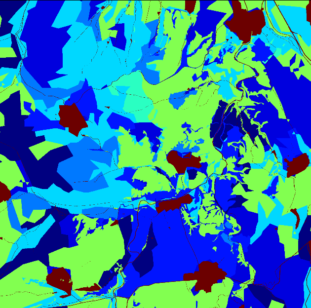
Figure 1: Fuel map of the simulation area. The colors are the 13 Anderson fuel categories.

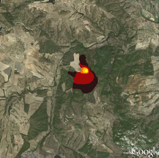
Figure 2: Burned area every 4 hours after the fire start.

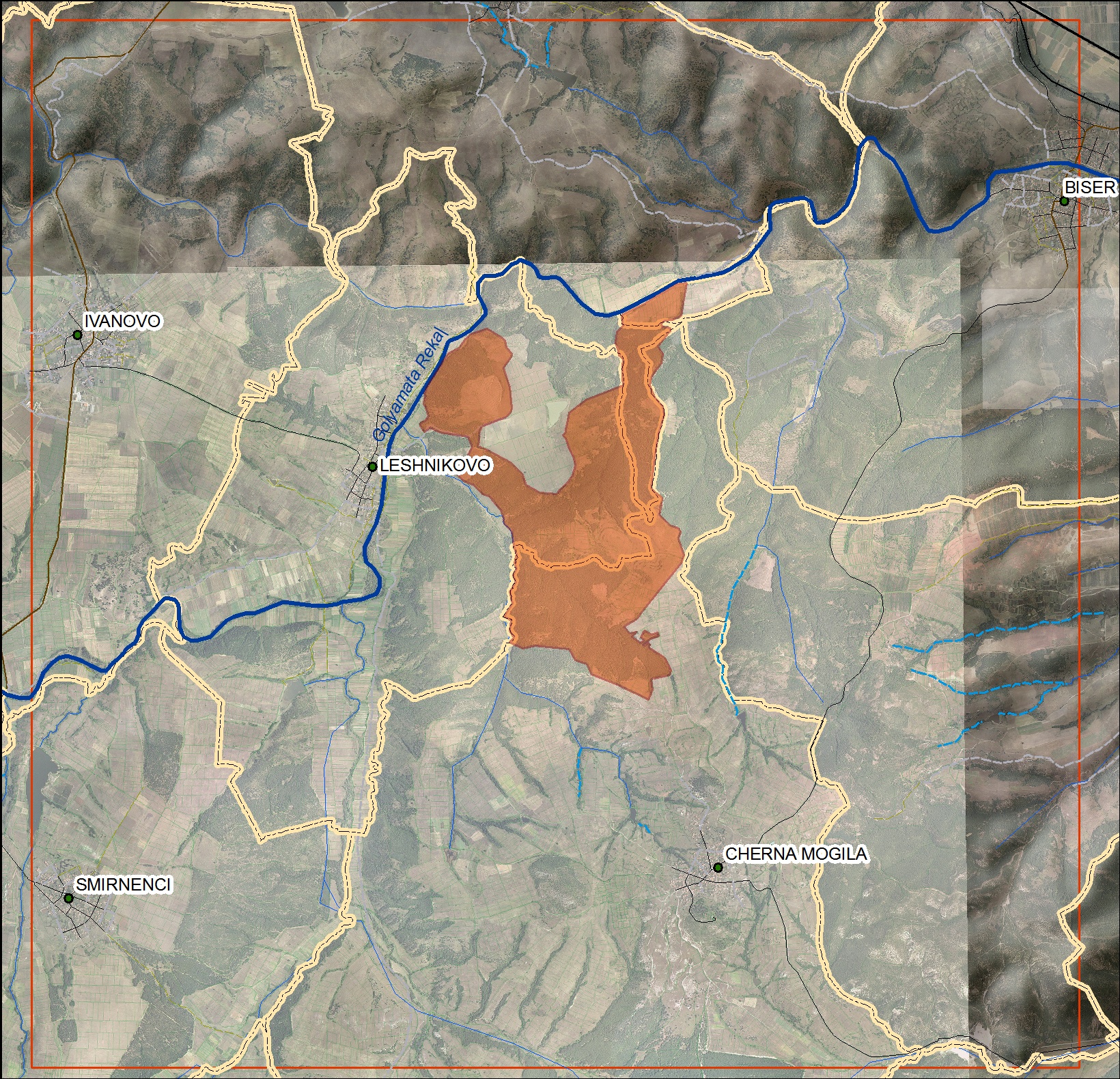
Figure 3: Map of the burned area and the fire perimeter.

Figure 4: The heat flux (red is high), the burned area (black), and the atmospheric flow (purple is over $10$m/s). Note the updraft caused by the fire. Ground image from Google Earth.

The data received from the server is a GIS raster format (DTED), which must first be processed and converted to geogrid’s binary data format. Using the powerful and open-source Quantum GIS (www.qgis.org), we open the downloaded raster and fill in the missing data with bilinear interpolation and project the data onto the Lambert Conformal Conic projection used in the model. Finally, we export the raster into a GeoTIFF file, which can be converted into the geogrid format using a utility included with the extended source distribution from openwfm.org, called convert_geotiff. This procedure is explained in detail at http://www.openwfm.org/wiki/How_to_run_WRF-Fire_with_real_data .

The final piece of surface data needed for input into geogrid is a categorical field describing the properties of the fuels. In the U.S., this data is readily available from the USGS; however, no such data exists for the Harmanli region. Instead, we create this field using data from the Corine Landcover Project (financed by the European Environment Agency and the member states). This project provides landcover data for Bulgaria with $100$ m resolution with a $25$ ha minimum mapping unit (http://www.eea.europa.eu/data-and-maps/data/corine-land-cover-2006-raster). We use downloaded data along with orthophoto data from the geoportal of the Ministry of Regional Development and Public Works (MRDPW) of Bulgaria to estimate the fuel behavior throughout the domain. All rivers, lakes, villages and forest areas have been vectorized using the orthophoto images combined with CORINE2006 into a GIS vector shape file. The vectorized file provides very high accuracy of representation for non burning areas like rivers and lakes as well as areas with high burning fuel level like woods. We assess the fuel behavior of every land cover category using data from the MRDPW and assign each area a fuel category using the 13 standard Anderson fuel models [8]. Table 1 gives a description of the fuel categories used in the Harmanli simulation.

This fuel level data combined with the vectorized landcover areas gives us a final shape file with attributes for each polygon fuel level. We again use Quantum GIS to rasterize the shape file into a $10$ m resolution GeoTIFF file, which we convert into the geogrid format as described above. Along with WPS’s standard global datasets, we place the newly created files in the WPS working directory and run the geogrid binary. The resulting input files contain all the standard WRF fields along with several additional variables generated from the high resolution topography and fuel categories.

4 Simulation results

The atmospheric model was run with two domains. The outer one with $250$m resolution consists of $180\times 180\times 41$ grid points, while the inner one with $50$m resolution consists of $221\times 221\times 41$ grid points. The fire model (coupled with the inner domain) runs with mesh step $5$m. The time step for the inner domain and the fire model was $0.3$s, while for the outer domain it was $1.5$s.

The fuel data is in Fig. 1. The simulated fire spread is shown in Fig. 2. The actual final burn area is shown in Fig. 3 for comparison. Fig. 4 shows the atmospheric flow above the fire.

Cores	6	12	24	36	60	120	240	360	480	720	960	1200
Fire	1.91	1.08	0.50	0.34	0.22	0.13	0.08	0.06	0.06	0.04	0.10	0.04
Inner domain	6.76	7.05	2.90	2.06	1.20	0.73	0.45	0.32	0.26	0.23	0.24	0.17
Outer domain	0.00	0.00	0.00	0.02	0.02	0.04	0.04	0.06	0.06	0.08	0.07	0.15
Total	10.59	9.21	3.91	2.75	1.64	0.99	0.61	0.44	0.37	0.31	0.44	0.26

Table 2: Execution times divided by simulation time for increasing number of processor cores. The fraction is given separately for the 3 components of the simulation: fire model and the two atmospheric model domains. The outer domain time includes communication between the atmospheric domains.

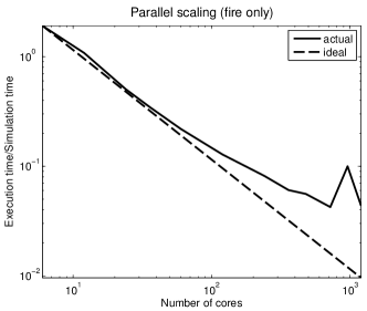
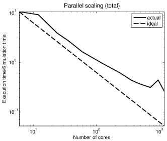
Figure 5: Parallel scalability data plotted from Table 2.

5 Parallel performance

The speed of the simulation is essential, because only a model that is faster than real time can be used for forecasting. We have performed computations on the Janus cluster at the University of Colorado. The computer consists of nodes with dual Intel X5660 processors (total 12 cores per node), connected by QDR InfiniBand. Table  2 and Figure 5 show that the coupled model is capable of running faster than real time, and the performance scales well with the number of processors. The model runs slightly faster than real time (1s of simulation time takes 0.99s to compute) on 120 cores.

6 Conclusion

We have demonstrated wildfire simulation based on real data in Bulgraria from satellite measurement and existing GIS databases. While the simulation provides a reasonable reproduction of the fire spread, further refinement is needed. Data assimilation [3, 9] will also play an important role. As seen from comparison of Figures 2 and 3, there is a good, but not not complete, agreement of the simulated and the real burned area. Despite this, the simulation showed correct fire line propagation, and it can give forecast and valuable information for future firefighting actions in different areas with different meteorological conditions. The model can perform faster than real time at the required resolution, thus satisfying one basic requirement for a future use for prediction.

Acknowledgements

This work was partially supported by the National Science Fund of the Bulgarian Ministry of Education, Youth and Science under Ideas Concourse Grant DID-02-29 “Modelling Processes with Fixed Development Rules (ModProFix),” ESF project number BG51PO001-3.3.04-33/28.08.2009, U.S. National Science Foundation (NSF) under grant AGS-0835579, and by U.S. National Institute of Standards and Technology Fire Research Grants Program grant 60NANB7D6144. Computational resources were provided by NSF grant CNS-0821794, with additional support from UC Boulder, UC Denver, and NSF sponsorship of NCAR.

References

- [1] Dobrinkova, N., Jordanov, G., Mandel, J.: WRF-Fire applied in Bulgaria. In Dimov, I., Dimova, S., Kolkovska, N., eds.: Numerical Methods and Applications. Volume 6046 of Lecture Notes in Computer Science. Springer, Berlin/Heidelberg (2011) 133–140
- [2] Mandel, J., Beezley, J.D., Kochanski, A.K.: Coupled atmosphere-wildland fire modeling with WRF-Fire version 3.3. Geoscientific Model Development Discussions 4 (2011) 497–545
- [3] Mandel, J., Beezley, J.D., Coen, J.L., Kim, M.: Data assimilation for wildland fires: Ensemble Kalman filters in coupled atmosphere-surface models. IEEE Control Systems Magazine 29 (2009) 47–65
- [4] Skamarock, W.C., Klemp, J.B., Dudhia, J., Gill, D.O., Barker, D.M., Duda, M.G., Huang, X.Y., Wang, W., Powers, J.G.: A description of the Advanced Research WRF version 3. NCAR Technical Note 475 (2008) http://www.mmm.ucar.edu/wrf/users/docs/arw_v3.pdf.
- [5] Rothermel, R.C.: A mathematical model for predicting fire spread in wildland fires. USDA Forest Service Research Paper INT-115 (1972) http://www.treesearch.fs.fed.us/pubs/32533.
- [6] Clark, T.L., Jenkins, M.A., Coen, J., Packham, D.: A coupled atmospheric-fire model: Convective feedback on fire line dynamics. J. Appl. Meteor. 35 (1996) 875–901
- [7] Clark, T.L., Coen, J., Latham, D.: Description of a coupled atmosphere-fire model. International Journal of Wildland Fire 13 (2004) 49–64
- [8] Anderson, H.E.: Aids to determining fuel models for estimating fire behavior. General Technical Report INT-122, US Department of Agriculture, Forest Service, Intermountain Forest and Range Experiment Station (1982) http://www.fs.fed.us/rm/pubs_int/int_gtr122.html.
- [9] Mandel, J., Beezley, J.D., Kondratenko, V.Y.: Fast Fourier transform ensemble Kalman filter with application to a coupled atmosphere-wildland fire model. In Gil-Lafuente, A.M., Merigo, J.M., eds.: Computational Intelligence in Business and Economics, Proceedings of MS’10. World Scientific (2010) 777–784 Also available as arXiv:1001.1588.